Propagating two-dimensional magnetic droplets

Abstract

Propagating, solitary magnetic wave solutions of the Landau-Lifshitz equation with uniaxial, easy-axis anisotropy in thin (two-dimensional) magnetic films are investigated. These localized, nontopological wave structures, parametrized by their precessional frequency and propagation speed, extend the stationary, coherently precessing “magnon droplet” to the moving frame, a non-trivial generalization due to the lack of Galilean invariance. Propagating droplets move on a spin wave background with a nonlinear droplet dispersion relation that yields a limited range of allowable droplet speeds and frequencies. An iterative numerical technique is used to compute the propagating droplet’s structure and properties. The results agree with previous asymptotic calculations in the weakly nonlinear regime. Furthermore, an analytical criterion for the droplet’s orbital stability is confirmed. Time-dependent numerical simulations further verify the propagating droplet’s robustness to perturbation when its frequency and speed lie within the allowable range.

and

1 Introduction

Magnetic materials yield a rich variety of intriguing nonlinear wave phenomena. Recent theoretical and experimental developments [1, 2, 3, 4] have enabled the controlled manipulation of magnetic moments on the nanometer length scale, the magnetic exchange length, thereby generating further interest in the field of nanomagnetism [5]. Dynamic, strongly nonlinear, localized wave structures varying on the exchange length scale have been studied theoretically for some time [6] (see the exhaustive review [7]). It was recently proposed that one member of this family of solitary waves, the two-dimensional (2D) nontopological droplet, could be experimentally realized in a spin torque nanocontact system that delivers a localized torque to a ferromagnetic thin film, balancing the inherent material damping [8]. The so-called dissipative droplet can, under certain conditions, experience a drift instability, propagating for some time before eventually succumbing to magnetic damping. A natural question arises, then, to inquire into the existence, stability, and properties of propagating, nontopological solitary waves in the underlying conservative model, the Landau-Lifshitz (LL) equation.

Previous studies of 2D propagating droplets include numerical computations in the isotropic [9] and anisotropic [10] regimes as well as weakly nonlinear asymptotics [11]. In [10], a numerical study of topological and nontopological localized solutions in 2D ferromagnets with easy-axis anisotropy was undertaken. Stationary droplets were constructed numerically which were then made to propagate in time-dependent simulations by the imposition of an initial, unidirectional phase gradient. The following approximate properties were observed: the excitation, accompanied by spin wave radiation, moved coherently with constant speed, a single frequency of precession, and a spatially dependent phase lag. In this work, we demonstrate that the excitations observed in [10] and the moving, coherent structures in [8] can be identified as propagating, nontopological droplet solitary waves which we construct directly by studying a nonlinear eigenvalue problem.

We undertake a careful numerical and asymptotic study of propagating 2D nontopological droplets, from here on in termed droplets. A two-parameter family of localized solitary wave solutions to the LL equation with easy-axis anisotropy parametrized by speed $V$ and rest frequency $\omega$ is constructed. In order to avoid a linear resonance, we are led to postulate the droplet’s existence and stability for speeds and frequencies in the restricted range

$$1-\omega-\frac{V^{2}}{4}>0,$$

similar to the existence conditions for moving 1D droplets [7, 12]. The droplet’s structure is studied analytically in the large amplitude, small speed regime and in the weakly nonlinear regime following [11]. A nonlinear dispersion relation for a background spin wave which modulates the propagating droplet naturally arises. It degenerates to the linear dispersion relation for exchange spin waves in the small amplitude regime where the Nonlinear Schrödinger equation approximately governs the dynamics. An iterative numerical method is employed to compute the droplet’s structure in the comoving frame by solving an appropriate boundary value problem. These results are used to compute the amplitude, asymmetry, energy, momentum, and more for a wide range of propagating droplets which agree with the asymptotic calculations. Droplet orbital stability is confirmed by numerical verification of an analytical, Jacobian condition. Time-dependent numerical simulations with initially perturbed propagating droplets further demonstrate the robustness of droplet propagation.

The outline of this work is as follows. In Sec. 2, several equivalent forms of the LL equation are introduced for later use in asymptotic and numerical analysis. In addition, properties of the stationary droplet are reviewed. The propagating droplet problem formulation and some basic properties are discussed in Sec. 3. Section 4 presents the asymptotic results. In Sec. 5, numerical results addressing droplet properties and stability are given. Further discussion and conclusions are related in Sec. 6 and 7. Finally, validation of the numerical technique is presented in the Appendix.

2 Model Equations and the Stationary Droplet

The Landau-Lifshitz torque equation

$$\frac{\partial\vec{M}}{\partial t}=-|\gamma|\mu_{0}\vec{M}\times\vec{H}_{\textrm{eff}}\,,$$ (1a)

$$\vec{H}_{\textrm{eff}} =$$ (1b)

$$~{}\frac{2A}{\mu_{0}M_{\mathrm{s}}^{2}}\Delta\vec{M}+\left(H_{0}+\frac{2K_{\mathrm{u}}}{\mu_{0}M_{\mathrm{s}}^{2}}M_{3}\right)\vec{e}_{3}+\vec{H}_{d}\,,$$

describes the dissipationless dynamics of the magnetization $\vec{M}:~{}\mathbb{R}^{2}\times[-\delta/2,\delta/2]\times\mathbb{R}^{+}\to M_{\mathrm{s}}\mathbb{S}^{2}$ in an unbounded ferromagnetic film of thickness $\delta$ exhibiting perpendicular, uniaxial anisotropy and a perpendicular applied magnetic field [13].

Relevant parameters for Eq. (1) are the gyromagnetic ratio ($\gamma$), the free space permeability ($\mu_{0}$), the exchange stiffness parameter ($A$), the perpendicular magnetic field amplitude ($H_{0}$), and the crystalline anisotropy constant ($K_{\mathrm{u}}$).

The magnetization

$$\vec{M}\equiv M_{\mathrm{s}}\vec{m}\equiv M_{\mathrm{s}}\sum_{j=1}^{3}m_{j}\,\vec{e}_{j}\,,$$ (2)

satisfies $|\vec{M}(\vec{x},t)|=M_{\mathrm{s}}$, where $M_{\mathrm{s}}$ is the saturation magnetization, as can be verified by taking the dot product of (1) with $\vec{M}$. The vectors $\vec{e}_{j}$, $j=1,2,3$, are the standard Cartesian basis vectors for $\mathbb{R}^{3}$ (see Fig. 1). The magnetostatic or dipolar field $\vec{H}_{d}$ is, in general, nonlocal, coupling the magnetization dynamics to Maxwell’s equations which, in the magnetostatic regime, take the form

$$\nabla\cdot\vec{H}_{d}=-\nabla\cdot\vec{M},$$

where $\vec{M}$ is extended to zero outside of $\mathbb{R}^{2}\times[-\delta/2,\delta/2]$. We are interested in the thin film regime where $\delta$ is sufficiently small. There are a number of different thin film scalings that depend upon the length scales inherent to the problem at hand. In the static case, some thin film limits have been rigorously justified via $\Gamma$-convergence; see, e.g., [14, 15] and references therein. Thin film magnetodynamics have also been rigorously studied [14, 16]. In many thin film scalings, there are two key simplifications that can be made: the magnetization is approximately uniform through the thickness of the film so that the problem is approximately 2D

$$\Delta\to\frac{\partial^{2}}{\partial x_{1}^{2}}+\frac{\partial^{2}}{\partial x_{2}^{2}},$$ (3)

and the dipolar field can be approximated by the local term

$$\vec{H}_{d}\to-M_{3}\vec{e}_{3}.$$ (4)

Heuristically, the two-dimensionality of the problem is justified when the film thickness is much smaller than the transverse magnetic excitations of interest because the exchange energy for magnetization variations in the $x_{3}$ direction would be prohibitively large. In our case, this amounts to the requirement

$$\delta\ll L_{ex}/(Q-1)^{1/2}\,,$$ (5)

where $L_{ex}$ is the magnetic exchange length

$$L_{ex}=\left(\frac{2A}{\mu_{0}M_{\mathrm{s}}^{2}}\right)^{1/2}\,,$$

typically on the order of several nanometers, and $Q$ is the dimensionless quality factor

$$Q=\frac{2K_{\mathrm{u}}}{\mu_{0}M_{\mathrm{s}}^{2}}\,,$$

assumed here to be greater than unity. Assuming that $\partial_{x_{3}}\vec{M}=0$, we can compute the 2D Fourier transform of the $x_{3}$ averaged dipolar field (see e.g. [17])

$$\begin{split}\widehat{(\vec{H}_{d}+M_{\mathrm{s}}\vec{e}_{3})}=&~{}-\frac{\vec{k}[\vec{k}\cdot\widehat{\vec{M}}_{\perp}(\vec{k})]}{k^{2}}[1-\widehat{\Gamma}(k\delta)]\\ &~{}-\widehat{(M_{3}-M_{\mathrm{s}})}(\vec{k})\,\widehat{\Gamma}(k\delta)\vec{e}_{3}\,,\end{split}$$ (6)

where $\widehat{f}(\vec{k})=\int_{\mathbb{R}^{2}}f(\vec{x}_{\perp})e^{-i\vec{k}\cdot\vec{x}_{\perp}}\,d\vec{x}_{\perp}$, $\vec{x}_{\perp}=(x_{1},x_{2})$, $\vec{M}_{\perp}=(M_{1},M_{2})$, and

$$\widehat{\Gamma}(k\delta)=\frac{1-e^{-k\delta}}{k\delta}\,.$$ (7)

The Fourier transforms are computed for rapidly decaying functions. In this work, we study solutions that rapidly decay to $\vec{M}\to M_{\mathrm{s}}\vec{e}_{3}$ with the decay length $L_{ex}/(Q-1)^{1/2}$ (see non-dimensionalization below). Then the Fourier transforms in (6) are concentrated on wavevectors $\vec{k}$ of order $(Q-1)^{1/2}/L_{ex}$ or less. Under the assumption (5), we can approximate (6), (7) as

$$\begin{split}\widehat{\Gamma}(k\delta)&\sim 1-\frac{1}{2}k\delta=1+\mathcal{O}\left(\delta\frac{(Q-1)^{1/2}}{L_{ex}}\right),\\ \vec{H}_{d}&=-M_{3}\vec{e}_{3}+\mathcal{O}\left(\delta\frac{(Q-1)^{1/2}}{L_{ex}}\right),\end{split}$$

hence (4) is justified.

It is convenient to nondimensionalize Eq. (1) according to (2) and

$$\begin{split}t^{\prime}&=|\gamma|\mu_{0}M_{\mathrm{s}}(Q-1)t\,,\quad\vec{x}^{\prime}=\frac{(Q-1)^{1/2}}{L_{ex}}\vec{x}\,,\\ h_{0}&=\frac{H_{0}}{M_{\mathrm{s}}(Q-1)},\end{split}$$ (8)

so that, after dropping primes, the problem of studying localized solutions to Eq. (1) subject to (3) and (4) becomes

$$\begin{split}&\frac{\partial\vec{m}}{\partial t}=-\vec{m}\times\left[\Delta\vec{m}+(m_{3}+h_{0})\,\vec{e}_{3}\right]\,\\ &\vec{m}:~{}\mathbb{R}^{2}\times\mathbb{R}^{+}\to\mathbb{S}^{2},\quad\lim_{|\vec{x}|\to\infty}\vec{m}(\vec{x},t)=\vec{e}_{3},\quad t\geq 0.\end{split}$$ (9)

The nondimensionalization (8) assumes an easy-axis anisotropy so that the quality factor $Q$, measuring the relative strength of the anisotropy to the magnetostatic energy, is larger than unity. When $Q<1$, the anisotropy is of the easy-plane variety. Anisotropic ferromagnetic nanostructures in this thin film geometry can be fabricated, e.g., using Cobalt/Nickel multilayers [5].

Transforming to the rotating frame

$$\begin{split}\vec{m}^{\prime}=[&m_{1}\,\cos{(h_{0}\,t)}+m_{2}\,\sin{(h_{0}\,t)},\\ &-m_{1}\sin{(h_{0}\,t)}+m_{2}\,\cos{(h_{0}\,t)},m_{3}],\end{split}$$

takes Eq. (9) to the parameterless form (after dropping the prime)

$$\frac{\partial\vec{m}}{\partial t}=-\vec{m}\times\vec{h}_{\textrm{eff}},\quad\vec{h}_{\textrm{eff}}=\Delta\vec{m}+m_{3}\,\vec{e}_{3}.$$ (10)

Therefore, without loss of generality, we will consider localized solutions of Eq. (10).

Equation (10) admits a family of localized, coherently precessing solutions [6, 7]. The solutions that incorporate a complete reversal of the magnetization, i.e. $\vec{m}(\vec{x}_{0},t)=\mp\vec{e}_{3}$ and $\lim_{|\vec{x}|\to\infty}\vec{m}(\vec{x},t)=\pm\vec{e}_{3}$ for one $\vec{x}_{0}\in\mathbb{R}^{2}$ (magnetic vortices), are called topological and exhibit pinning of the soliton center, hence cannot propagate [18]. In contrast, solutions that do not exhibit magnetization reversal are termed nontopological and can propagate. Such solutions are the focus of this work.

Sufficiently localized solutions of Eq. (10) conserve the magnetic energy

$${\cal E}[\vec{m}]=\frac{1}{2}\int\left[\left|\nabla\vec{m}\right|^{2}+\left(1-m_{3}^{2}\right)\right]\,\mathrm{d}\vec{x}\,,$$ (11)

which incorporates contributions due to exchange $|\nabla\vec{m}|^{2}$ and anisotropy $(1-m_{3}^{2})$. Integration is always assumed to be taken over the plane $\mathbb{R}^{2}$ unless otherwise noted. The effective field in Eq. (10) is derived from the magnetic energy via

$$\vec{h}_{\textrm{eff}}=-\frac{\delta\mathcal{E}}{\delta\vec{m}}\,.$$

Figure 1: Schematic of the coordinate systems for a planar ferromagnet consisting of the domain of $\vec{m}$ ($\mathbb{R}^{2}$ in polar coordinates with radius $\rho$, azimuthal angle $\varphi$) and the range of $\vec{m}$ (unit sphere $\mathbb{S}^{2}$ with polar angle $\Theta$, azimuthal angle $\Phi$).

Other conserved quantities include the spin density

$$\mathcal{N}[\vec{m}]=\int(1-m_{3})\,\mathrm{d}\vec{x},$$ (12)

and the momentum

$$\boldsymbol{\mathcal{P}}[\vec{m}]=\int\frac{m_{2}\nabla m_{1}-m_{1}\nabla m_{2}}{1+m_{3}}\,\mathrm{d}\vec{x}.$$ (13)

The quantity ${\cal N}$ can be interpreted as the mean number of spin deviations from the uniform state $\vec{e}_{3}$ in a localized magnetic excitation. In the quantum limit it takes integer values and corresponds to the number of magnons in an excited ferromagnet [7].

Note that the momentum as given in (13) is ambiguous when the magnetization involves topological structures. The ambiguity has been addressed by considering moments of the topological vorticity [18]. Since we are considering nontopological structures, the momentum in (13) is equivalent to the more general formulation of [18].

Small amplitude exchange spin waves deviating from the background state $\vec{e}_{3}$ in the form

$$\begin{split}m_{1}&=\varepsilon\cos(\vec{k}\cdot\vec{x}-\omega_{\textrm{L}}t),\\ m_{2}&=-\varepsilon\sin(\vec{k}\cdot\vec{x}-\omega_{\textrm{L}}t)],\quad m_{3}\sim 1,\quad|\varepsilon|\ll 1\,,\end{split}$$

with wavenumber $\vec{k}$ and frequency $\omega_{\textrm{L}}$ satisfy the linear dispersion relation

$$\omega_{\textrm{L}}(\vec{k})\equiv\omega_{\textrm{L}}(k)=1+k^{2}\,,\quad k=|\vec{k}|\,.$$ (14)

2.1 Alternate Forms of the Landau-Lifshitz Equation

Two alternative forms for Eq. (10) will be used in this work. For the first, we use the spherical basis (see Fig. 1)

$$\vec{m}=[\cos{\Phi}\,\sin{\Theta},\sin{\Phi}\,\sin{\Theta},\cos{\Theta}],$$

where $\Phi\in[0,2\pi)$ $(\textrm{mod}\,2\pi)$ and $\Theta\in[0,\pi]$ are the azimuthal and polar angles, respectively. Inserting this expression into Eq. (10) gives

$$\frac{\partial\Theta}{\partial t}=F[\Theta,\Phi]\,,\qquad\sin{\Theta}\frac{\partial\Phi}{\partial t}=G[\Theta,\Phi]\,,$$ (15a)

where

$$\begin{split}F[\Theta,\Phi]&=\frac{\nabla\cdot\left(\sin^{2}{\Theta}\,\nabla\Phi\right)}{\sin{\Theta}},\\ G[\Theta,\Phi]&=\frac{1}{2}\,\sin(2\Theta)\,(|\nabla\Phi|^{2}+1)-\Delta\Theta\,.\end{split}$$ (15b)

We will see that Eq. (15) is in a useful form to study stationary and slowly moving droplets as well as to formulate an energy minimization problem for propagating droplets. The energy, spin density, and momentum in these variables take the form

$${\cal E}[\Theta,\Phi] =\frac{1}{2}\int\left[\left|\nabla\Theta\right|^{2}+\sin^{2}{\Theta}\,\left(1+\left|\nabla\Phi\right|^{2}\right)\right]\,\mathrm{d}\vec{x}\,,$$ (16a)

$$\mathcal{N}[\Theta] =\int\left(1-\cos{\Theta}\right)\,\mathrm{d}\vec{x}\,,$$ (16b)

$$\boldsymbol{\mathcal{P}}[\Theta,\Phi] =\int\left(\cos{\Theta}-1\right)\,\nabla{\Phi}\,\mathrm{d}\vec{x}\,.$$ (16c)

Note that (15) is Hamilton’s equations in the form

$$\frac{\partial\Phi}{\partial t}=-\frac{\delta\mathcal{E}}{\delta\cos{\Theta}},\quad\frac{\partial\cos{\Theta}}{\partial t}=\frac{\delta\mathcal{E}}{\delta\Phi},$$

where $\Phi$ and $\cos{\Theta}$ are the canonically conjugate variables for the Hamiltonian system.

Another representation of (10) can be had by performing the stereographic projection

$$w=\frac{m_{1}+im_{2}}{1+m_{3}}=\frac{e^{i\Phi}\sin{\Theta}}{1+\cos{\Theta}}.$$ (17)

Then (10) becomes [19]

$$i\,w_{t}=\Delta w-\frac{2w^{*}\nabla w\cdot\nabla w+w(1-|w|^{2})}{1+|w|^{2}}\,,$$ (18)

where the appended asterisk denotes complex conjugation. This form of the LL equation is amenable to weakly nonlinear asymptotics (Sec. 4) and numerical analysis (Sec. 5). The conserved quantities are

$${\cal E}[w] =2\int\frac{\left|\nabla w\right|^{2}+|w|^{2}}{\left(1+|w|^{2}\right)^{2}}\,\mathrm{d}\vec{x}\,,$$ (19a)

$$\mathcal{N}[w] =2\int\frac{|w|^{2}}{1+|w|^{2}}\,\mathrm{d}\vec{x}\,,$$ (19b)

$$\boldsymbol{\mathcal{P}}[w] =-2\int\frac{\textrm{Im}(w^{*}\nabla w)}{1+|w|^{2}}\,\mathrm{d}\vec{x}\,.$$ (19c)

In analogy with a Bose-Einstein condensate [20], the momentum (19c) corresponds to a weighted phase gradient or a “magnetic superfluid” momentum.

For the time-dependent initial value problem discussed in Sec. 5.3, we will solve Eq. (10). Thus, we will make use of all three forms (10), (15), and (17) of the LL equation in our analysis.

2.2 Stationary Droplet

An azimuthally symmetric, stationary, localized droplet solution to the LL equation was studied in [6, 7]. We note that the term magnon droplet was used because of its analogy with a localized “droplet” of a condensed, attractive one-dimensional Bose gas [7]. In this section, we briefly review the properties of the stationary droplet.

It is convenient to write the stationary droplet solution in a spherical basis satisfying Eq. (15). It takes the form

$$\begin{split}&\Theta(\vec{x},t)=\Theta_{0}(\rho;\omega)\,,\quad\Phi(\vec{x},t)=\omega\,t\,,\\ &F[\Theta_{0},\omega\,t]=0\,,\quad G[\Theta_{0},\omega t]=\omega\,\sin{\Theta_{0}}\,,\end{split}$$

where $\rho=\sqrt{x_{1}^{2}+x_{2}^{2}}$ is the distance from the origin and the polar angle function $\Theta_{0}$, parametrized by the droplet frequency $\omega$, is determined by solving the following nonlinear eigenvalue problem

$$-\left(\frac{\mathrm{d}^{2}}{\mathrm{d}\rho^{2}}+\frac{1}{\rho}\frac{\mathrm{d}}{\mathrm{d}\rho}\right)\Theta_{0}+\sin{\Theta_{0}}\,\cos{\Theta_{0}}-\omega\sin{\Theta_{0}}=0\,,$$ (20a)

$$\frac{\mathrm{d}\Theta_{0}}{\mathrm{d}\rho}(0;\omega)=0\,,\quad\lim_{\rho\to\infty}\Theta_{0}(\rho;\omega)=0\,.$$ (20b)

The ground state solution that is positive and monotonically decaying is sought. One can show that $0<\Theta_{0}(\rho;\omega)<\pi$, therefore this solution is termed non-topological [7]. In contrast, there exist topological droplets that satisfy a related nonlinear eigenvalue problem with the conditions $\Theta_{0}(0;\omega)=\pi$, $\Theta_{0}(\rho;\omega)\to 0$. Their existence and stability subject to certain symmetric perturbations were studied rigorously in [21].

Assuming the existence of a localized solution, the following inequality holds

$$0<\omega<1\,,$$ (21)

which can be seen by multiplying Eq. (20a) by $\frac{\mathrm{d}\Theta_{0}}{\mathrm{d}\rho}\,\rho^{2}$ and integrating to find

$$2\,\omega\int_{0}^{\infty}\left(1-\cos{\Theta_{0}}\right)\,\rho\,\mathrm{d}\rho-\int_{0}^{\infty}\sin^{2}{\Theta_{0}}\,\,\rho\,\mathrm{d}\rho=0.$$ (22)

We immediately observe that

$$\omega=\frac{\int_{0}^{\infty}\sin^{2}{\Theta_{0}}\,\,\rho\,\mathrm{d}\rho}{2\int_{0}^{\infty}(1-\cos{\Theta_{0}})\,\rho\,\mathrm{d}\rho}>0\,.$$

Using the fact that $2\,(1-\cos{\Theta})>\sin^{2}{\Theta}$ for $0<\Theta<\pi$, we also have $\omega<1$.

The decay rate of $\Theta_{0}$ can be obtained by expanding (20a) for large values of $\rho$ and neglecting nonlinear terms which gives

$$-\frac{\mathrm{d}^{2}\Theta_{0}}{\mathrm{d}\rho^{2}}-\frac{1}{\rho}\frac{\mathrm{d}\Theta_{0}}{\mathrm{d}\rho}+(1-\omega)\,\Theta_{0}\sim 0\,,$$

giving

$$\Theta_{0}(\rho)=\mathcal{O}\left(\frac{e^{-\rho\,\sqrt{1-\omega}}}{\sqrt{\rho}}\right)\,,\quad\rho\gg 1\,.$$ (23)

From numerical computations, see, e.g., [10], it is known that the amplitude of the droplet increases with decreasing frequency. As the frequency approaches zero, the droplet resembles a circular domain wall with a transition layer that moves further away from the droplet center. The nonlinear, orbital stability of nontopological, three-dimensional solitary waves in the context of anisotropic, two sublattice ferrites were studied by use of a Lyapunov functional whose positive definiteness is guaranteed when [22]

$$\frac{\d\mathcal{N}}{\d\omega}<0\,,$$ (24)

which is commonly referred to as a slope or VK condition after Vakhitov-Kolokolov’s work on Nonlinear Schrödinger solitary waves [23]. Since $\mathcal{N}^{\prime}(\omega)$ is the Jacobian of the map from the physical variable $\omega$ to the conserved quantity $\mathcal{N}$, we refer to (24) as a Jacobian condition as this will naturally generalize to the stability criterion for propagating droplets. The Jacobian condition (24) has been numerically verified for 2D stationary droplets [7], suggesting their orbital stability. Their robustness to perturbations in 2D, time-dependent numerical simulations [8] are further evidence of their stability.

3 Propagating Droplet: Problem Formulation and Basic Results

A two-parameter family of moving droplet solutions of (15) is considered in the form

$$\Theta(\vec{x},t)=\theta(\boldsymbol{\xi};\omega,\vec{V})\,,$$ (25a)

$$\Phi(\vec{x},t)=\omega t+\phi(\boldsymbol{\xi};\omega,\vec{V})\,,$$ (25b)

with

$$\boldsymbol{\xi}=\vec{x}-\vec{V}\,t\,,$$ (25c)

where $\omega$ is the droplet’s rest frequency and $\vec{V}$ is the droplet’s velocity. Insertion of this ansatz into Eq. (15) results in

$$\sin{\theta}\,\left(\omega-\vec{V}\cdot\nabla\phi\right)=\\ -\Delta\theta+\sin{\theta}\,\cos{\theta}\,\left(1+|\nabla\phi|^{2}\right)\,,$$ (26a)

$$-\sin{\theta}\,\vec{V}\cdot\nabla\theta=\nabla\cdot\left(\sin^{2}\theta\,\nabla\phi\right).$$ (26b)

The propagating nontopological droplet that we seek satisfies the boundary conditions

$$\lim_{|\boldsymbol{\xi}|\to\infty}\theta(\boldsymbol{\xi};\omega,\vec{V})=0\,,\,\,\lim_{|\boldsymbol{\xi}|\to\infty}\nabla\phi(\boldsymbol{\xi};\omega,\vec{V})=\textrm{const}\,,$$ (27)

with $\theta(\boldsymbol{\xi};\omega,\vec{V})<\pi$ for all $\boldsymbol{\xi}\in\mathbb{R}^{2}$. Assuming decay for $|\boldsymbol{\xi}|$ sufficiently large, $\theta\ll 1$ and $\nabla\phi\sim\vec{U}$ a constant vector, Eq. (26b) is asymptotically

$$-\vec{V}\cdot\nabla\theta=2\vec{U}\cdot\nabla\theta\,.$$

Therefore,

$$\lim_{|\boldsymbol{\xi}|\to\infty}\nabla\phi(\boldsymbol{\xi};\omega,\vec{V})=-\frac{\vec{V}}{2}\,.$$ (28)

Due to the $SO(2)$ invariance of the LL equation (10), it is sufficient to consider

$$\vec{V}=V\vec{e}_{1},\quad V>0\,.$$ (29)

For the rest of this work, expression (29) is assumed to hold.

By use of (16), we observe that (26) is equivalent to the following

$$\frac{\delta}{\delta\theta}\left(\omega\,\mathcal{N}+V\,\mathcal{P}_{1}\right) =\frac{\delta\mathcal{E}}{\delta\theta}\,,$$ (30a)

$$\frac{\delta}{\delta\phi}\left(\omega\,\mathcal{N}+V\,\mathcal{P}_{1}\right) =\frac{\delta\mathcal{E}}{\delta\phi}\,,$$ (30b)

where $\mathcal{P}_{1}$ is the nonvanishing component of $\vec{\mathcal{P}}$ when condition (29) holds. Equations (30) are the necessary conditions for a minimizer of the functional

$$\mathcal{D}[\theta,\phi]=\mathcal{E}[\theta,\phi]-\omega\mathcal{N}[\theta,\phi]-V\mathcal{P}_{1}[\theta,\phi]\,,$$ (31)

where $\omega$ and $V$ are Lagrange multipliers ensuring the constraints of fixed spin density $\mathcal{N}$ and momentum $\mathcal{P}_{1}$. Propagating, localized structures in 2D isotropic [9] and 3D anisotropic [24] ferromagnets were studied numerically by minimizing a similar functional. Note that,

$$\mathcal{N}=-\frac{\partial\mathcal{D}}{\partial\omega}\,,\quad\mathcal{P}_{1}=-\frac{\partial\mathcal{D}}{\partial V}\,.$$ (32)

While the variational formulation of the droplet leads to a parameterization in terms of $\mathcal{N}$ and $\mathcal{P}_{1}$, for physical applications, it is natural to parameterize the droplet in terms of the physical variables $\omega$ and $V$. Solving Eqs. (26) for fixed $\omega$ and $V$ provides the map $(\omega,V)\mapsto(\mathcal{N},\mathcal{P}_{1})$. Invertibility of this map requires that the Jacobian

$$J=\frac{\partial\mathcal{P}_{1}}{\partial V}\frac{\partial\mathcal{N}}{\partial\omega}-\frac{\partial\mathcal{N}}{\partial V}\frac{\partial\mathcal{P}_{1}}{\partial\omega}\,,$$ (33)

be nonzero. In the context of other magnetic and nonlinear wave models, the orbital stability of two-parameter solitary waves is determined by the Jacobian condition [25, 26]

$$J<0\,.$$ (34)

Note that the Jacobian condition (34) degenerates to the Jacobian condition (24) for stationary droplets when $V=0$ because $\partial_{\omega}\mathcal{P}_{1}=0$ and $\partial_{V}\mathcal{P}_{1}>0$. Droplet stability will be discussed further in Secs. 4.1 and 5.3.

If $\theta_{*}(\boldsymbol{\xi})$, $\phi_{*}(\boldsymbol{\xi})$ are a minimizer of (31), then dilation of $\boldsymbol{\xi}$ by the factor $\lambda$ gives

$$d(\lambda)=\mathcal{D}[\theta_{*}(\lambda\cdot),\phi_{*}(\lambda\cdot)]\,.$$

A necessary condition for $\theta_{*}(\boldsymbol{\xi})$, $\phi_{*}(\boldsymbol{\xi})$ to be a minimum of (31) is therefore

$$d^{\prime}(1) =\int\sin^{2}{\theta_{*}}\,\,\mathrm{d}\boldsymbol{\xi}-V\,\mathcal{P}_{1}-2\,\omega\,\mathcal{N}=0\,,$$ (35)

which can be derived more generally by direct manipulation of conservation laws for the Landau-Lifshitz equation [27]. Similar identities were studied by Derrick [28] and Pohozaev [29]. We will make use of this relation in order to verify the validity of our numerical computations in the Appendix.

Another formulation of the boundary value problem (26), (27), (28) can be derived by considering Eq. (18) with a traveling wave solution in the form

$$w(x_{1},x_{2},t) =f(x_{1}-V\,t,x_{2})\,e^{i\,\omega\,t}$$

$$=f(\xi_{1},\xi_{2})\,e^{i\,\omega\,t}\,.$$ (36)

Inserting the ansatz (3) into Eq. (18) leads to the following nonlinear eigenvalue problem

$$\omega\,f+i\,Vf_{\xi_{1}}+f_{\xi_{1}\xi_{1}}+f_{\xi_{2}\xi_{2}}\\ -\frac{2f^{*}(f_{\xi_{1}}^{2}+f_{\xi_{2}}^{2})}{1+|f|^{2}}-f\frac{1-|f|^{2}}{1+|f|^{2}}=0\,,$$ (37)

with $f\to 0$ as $|\boldsymbol{\xi}|\to\infty$. Letting

$$f(\xi_{1},\xi_{2})=u(\xi_{1},\xi_{2})\,e^{-i\,\frac{V}{2}\,\xi_{1}}\,,$$

then (37) becomes

$$\begin{split}\omega\,u&+\frac{V^{2}}{4}u+u_{\xi_{1}\xi_{1}}+u_{\xi_{2}\xi_{2}}\\ &-\frac{2u^{*}[(u_{\xi_{1}}-i\frac{V}{2}u)^{2}+u_{\xi_{2}}^{2}]}{1+|u|^{2}}-u\frac{1-|u|^{2}}{1+|u|^{2}}=0\,.\end{split}$$ (38)

We observe that for $V\neq 0$, $u$ is generally complex-valued. Assuming localization and linearizing Eq. (38) for $|\boldsymbol{\xi}|\to\infty$, we obtain

$$u_{\xi_{1}\xi_{1}}+u_{\xi_{2}\xi_{2}}+\left(\omega+\frac{V^{2}}{4}-1\right)u=0\,.$$

Therefore, a necessary condition for localization is

$$\nu^{2}(V,\omega)>0,\quad\nu(V,\omega)=\left(1-\omega-\frac{V^{2}}{4}\right)^{1/2}\,,$$ (39)

and the exponential decay rate of $u$ is $\nu(V,\omega)$. We discuss the consequences of this observation in the next section.

3.1 The nonlinear dispersion relation

From the boundary condition in (28), we observe that the propagating droplet is modulated by a spin wave background with wave number

$$k=\frac{V}{2}\,,$$ (40)

and frequency in the laboratory frame

$$\omega_{\textrm{NL}}(k,\omega)=\omega+\frac{V^{2}}{2}=\omega+2k^{2}\,.$$ (41)

In contrast to the linear dispersion relation for exchange spin waves in (14), the nonlinear droplet dispersion relation in (41) depends on both the rest frequency $\omega$ and the speed $V$. The condition (39) corresponds to a negative nonlinear frequency shift

$$\omega_{\textrm{L}}(k)-\omega_{\textrm{NL}}(k,\omega)=1-\omega-k^{2}=\nu^{2}(V,\omega)>0.$$

This yields an upper bound on the droplet’s speed for a given rest frequency

$$0<V<V_{\textrm{max}}(\omega)=2\sqrt{1-\omega},$$

or, equivalently, an upper bound on the rest frequency for fixed speed

$$\omega<\omega_{\textrm{max}}(V)=1-\frac{V^{2}}{4}\,,\quad V>0.$$ (42)

In the limit $\omega\rightarrow 1$, condition (42), via (40), requires that $k\rightarrow 0$. The nonlinear dispersion relation (41) then coincides with the linear dispersion relation (14) for a spatially uniform, small amplitude excitation at the bottom of the spin wave band. Alternatively, in the limit $k\rightarrow k_{\mathrm{max}}\equiv\sqrt{1-\omega}$, we observe that $\omega_{NL}(k,\omega)\to 2-\omega=\omega_{L}(k_{\mathrm{max}})$ corresponding to a propagating exchange spin wave. The speed $V$ of the moving droplet is the group velocity $V_{g}$ of the background spin wave, $V_{g}=\mathrm{d}\,\omega_{\textrm{L}}/\mathrm{d}\,k=2\,k=V$. The phase speed of the background spin wave $\omega_{\textrm{L}}/k=\omega/k+2k$ can be greater than (when $\omega>0$) or less than (when $\omega<0$) the droplet traveling wave speed $V=2k$. In this work, we focus on the case $\omega>0$.

The dispersion relations are illustrated in the laboratory frame and the comoving droplet frame in Fig. 2. The shaded regions correspond to the localization condition (39) hence localized, propagating droplets can be interpreted as nonlinear bound states lying below the linear spin wave band [7].

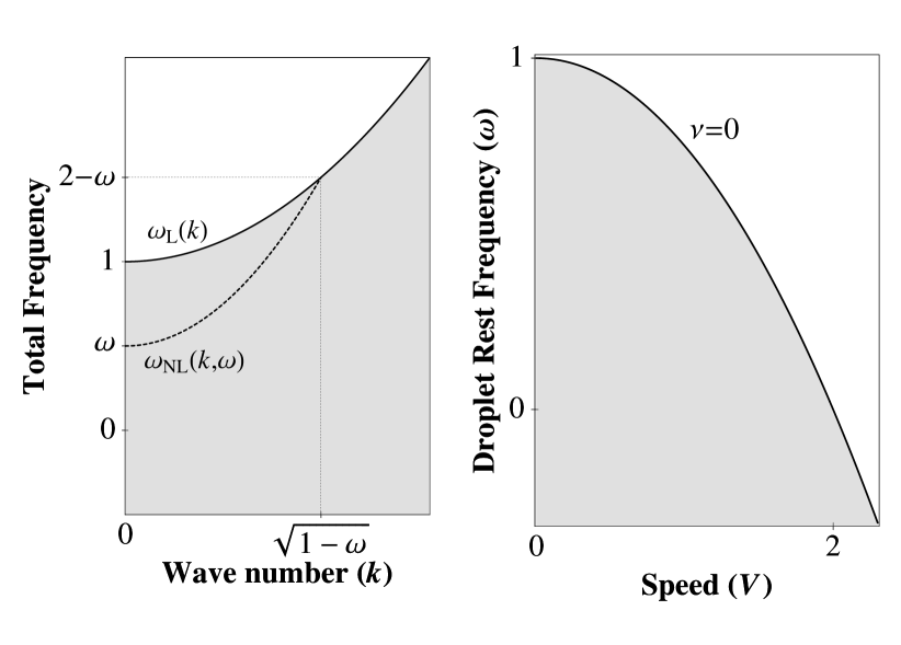
Figure 2: Dispersion relations in the laboratory frame (left) and the comoving droplet frame (right) with wavenumber $k=V/2$. The shaded regions represent accessible droplet solutions.

3.2 1D Droplet

The nonlinear dispersion relation in Eq. (41) for a 2D propagating droplet is the same for a propagating 1D droplet [7]. As will be shown, a number of 2D droplet properties are qualitatively similar to the 1D droplet properties. Therefore, in this section we briefly review some basic results about moving droplet solutions of the LL equation in (1+1) dimensions.

The Landau-Lifshitz Eq. (10) in one dimension, $\Delta\to\partial_{xx}$, is solvable by means of the inverse scattering transform (see, e.g., [30] and references therein) and admits soliton solutions. The single droplet soliton solution can be written as follows (see [12])

$$\cos\Theta= ~{}\frac{V^{2}-2+3\omega+\sqrt{V^{2}+\omega^{2}}\cosh[2\nu\xi]}{2-\omega+\sqrt{V^{2}+\omega^{2}}\cosh[2\nu\xi]}$$ (43a)

$$\Phi= ~{}\omega t-\frac{V\xi}{2}$$

$$+\tan^{-1}\left[\frac{4\nu\tanh(\nu\xi/2)}{V^{2}+2(\omega+\sqrt{V^{2}+\omega^{2}})}\right]\,,$$ (43b)

where $\xi=x-V\,t$ and $\nu$ is given in (39). Thus, the 1D soliton solution exists for all $V>0$, $\omega$ satisfying (39). When $V=0$, the rest frequency is limited to the unit interval (21). For $\omega<0$, $V=0$, the soliton (43) exhibits a phase singularity at the origin corresponding to topological behavior in this one dimensional setting. However, for $V>0$, the necessary condition $\omega<\omega_{\mathrm{max}}(V)$ in (42) has no lower bound. Therefore, nontopological solitons with arbitrarily negative rest frequencies exist even with vanishingly small propagation speeds. The phase gradient (43b) has the asymptotics

$$\Phi_{\xi}(0)\sim\frac{-V}{\omega+|\omega|+V^{2}/(2|\omega|)},\quad 0<\frac{V}{|\omega|}\ll 1,$$

hence can be quite large when $\omega<0$. Our numerical method for computing 2D propagating droplets fails for modes with large momentum due to large phase gradients (see Sec. 5.2) so we are limited in exploring this regime of parameter space in the two dimensional case.

Explicit expressions for the energy ${\cal{E}}^{(\mathrm{1D})}$, the spin density ${\cal{N}}^{(\mathrm{1D})}$ and the momentum ${\cal{P}}^{(\mathrm{1D})}$, as functions of $V$ and $\omega$, for a single moving droplet solution, can be obtained from solution (43) via Eqs. (11), (12) and (13):

$${\cal{E}}^{(\mathrm{1D})} =2\,\sqrt{4-4\,\omega-V^{2}}\,,$$

$${\cal{N}}^{(\mathrm{1D})} =2\,\tanh^{-1}{\left(\frac{\sqrt{4-4\,\omega-V^{2}}}{2-\omega}\right)}\,,$$

$${\cal{P}}^{(\mathrm{1D})} =\pi-2\,\tan^{-1}{\left(\frac{V^{2}+2\,\omega}{V\,\sqrt{4-4\,\omega-V^{2}}}\right)}\,.$$

We observe the notable fact that the momentum ${\cal{P}}^{(\mathrm{1D})}$ is bounded, $0\leq{\cal{P}}^{(\mathrm{1D})}<2\,\pi$, but the energy and spin density are not.

4 Propagating Droplet: Asymptotic Results

In this section, asymptotic methods are employed to study the behavior of the propagating droplet in the small amplitude and small speed regimes.

4.1 Weakly nonlinear regime

Small amplitude, propagating droplets were studied asymptotically in [11]. In this section, we briefly review the results with a view toward their numerical verification in Sec. 5.

Using a slowly varying envelope, small amplitude approximation the authors in [11] construct a propagating droplet bifurcating from the set of linear waves where the small parameter is the deviation from the linear band edge (39)

$$0<\nu(V,\omega)^{2}\ll 1\,.$$

The droplet solution for Eq. (18) takes the approximate form

$$\begin{split}w(x_{1},x_{2},t)&\sim\frac{\nu(V,\omega)}{\sqrt{2(2-\omega)}}e^{-i\left[V(x_{1}-V\,t)/2-\omega t\right]}\\ \times u_{T}&\left(\nu(V,\omega)\left[(x_{1}-V\,t)^{2}+x_{2}^{2}\right]^{1/2}\right)\,,\end{split}$$ (44)

with $\nu>0$ having the meaning of the inverse half width. As the band edge is approached, $\nu\to 0$, the propagating droplet is approximately a wide, small amplitude, propagating Townes mode [31], the unique, positive, monotonically decaying solution of

$$\begin{split}-u_{T}^{\prime\prime}-&\frac{1}{R}u_{T}^{\prime}-u_{T}^{3}+u_{T}=0\,,\\ u_{T}^{\prime}(0)&=0,\quad\lim_{R\to\infty}u_{T}(R)=0\,.\end{split}$$

Using (44) and its next order correction, the functional (31) can be expanded as [11]

$$\mathcal{D}\sim\frac{\mathcal{N}_{T}}{1+V^{2}/4}\left[\nu^{2}+\nu^{4}\frac{b(1-V^{2}/4)}{2(1+V^{2}/4)^{2}}\right]\,,$$ (45)

where

$$\begin{split}\mathcal{N}_{T}&\equiv\|u_{T}\|_{L^{2}(\mathbb{R}^{2})}^{2}\approx 11.7009\,,\\ b&\equiv\frac{2\pi\int_{0}^{\infty}u_{T}^{2}{u_{T}^{\prime}}^{2}R\,\mathrm{d}R}{\mathcal{N}_{T}}\approx 1.35825\,.\end{split}$$

Combining (45) with the relations (32), the propagating droplet’s spin density, momentum, and energy in the weakly nonlinear regime are approximately

$$\mathcal{N} \sim\frac{\mathcal{N}_{T}}{1+V^{2}/4}\left[1+\nu^{2}\frac{b(1-V^{2}/4)}{(1+V^{2}/4)^{2}}\right]$$ (46a)

$$\mathcal{P}_{1} \sim\frac{\mathcal{N}_{T}V}{2(1+V^{2}/4)}\bigg{[}1+\nu^{2}\bigg{(}b\frac{1-V^{2}/4}{(1+V^{2}/4)^{2}}$$ (46b)

$$\qquad\qquad\qquad\qquad\quad+\frac{1}{1+V^{2}/4}\bigg{)}\bigg{]}\,,$$

$$\mathcal{E} \sim\mathcal{N}_{T}\bigg{[}1+\nu^{2}\bigg{(}\frac{2b(1-V^{2}/4)}{(1-V^{2}/4)^{3}}$$ (46c)

$$\qquad\qquad\qquad+\frac{1+3V^{2}/4}{(1+V^{2}/4)^{2}}-\frac{1}{1+V^{2}/4}\bigg{)}\bigg{]}\,.$$

These results are numerically verified in Sec. 5.2.

For the initial value problem in the weakly nonlinear regime, one can derive at leading order the time-dependent cubic Nonlinear Schrödinger equation (NLS) from Eq. (18) for the slowly varying envelope of a carrier wave. In two spatial dimensions, the NLS equation exhibits critical blow up with the Townes mode playing an important role [32]. For initial data with $L^{2}(\mathbb{R}^{2})$ norm less than $\|u_{T}\|_{2}$, the solution disperses to zero as $t\to\infty$. In other cases, e.g. for data close to $u_{T}$ in $L^{2}(\mathbb{R}^{2})$ but with larger norm, the solution blows up in finite time. Thus, the Townes mode is unstable to small perturbations. It is natural then to inquire into the stability of the propagating droplet for the LL Eq. (18). The Jacobian condition (34) was verified in [11]. Insertion of (46a) and (46b) into Eq. (33), leads to

$$J=-\frac{b\omega\mathcal{N}_{T}}{2(2-\omega)^{4}}+\mathcal{O}(\nu^{2})\,,$$ (47)

suggesting that the higher order corrections to the NLS approximation stabilize the propagating droplet. Further discussion of stability in the large amplitude case is presented in Sec. 5.3.

4.2 Small propagation speed

We now consider Eqs. (26a) and (26b) with boundary conditions (27) and (28) for small values of the droplet speed $0<V\ll 1$. Polar coordinates are used (see Fig. 1)

$$\xi_{1}=x_{1}-Vt=\rho\,\cos{\varphi}\,,\quad\xi_{2}=x_{2}=\rho\,\sin{\varphi}\,.$$ (48)

A solution is sought in the form

$$\begin{split}\theta&=\Theta_{0}(\rho;\omega)+\mathcal{O}(V^{2})\,,\\ \phi&=V\,\left(\Phi_{1}(\rho,\varphi)-\frac{1}{2}\,\rho\,\cos{\varphi}\right)+\mathcal{O}(V^{2})\,,\end{split}$$ (49)

where $\Theta_{0}$ is the solution of Eq. (20) for the stationary droplet with $0<\omega<1$ and $\theta$ and $\phi$ are given in the ansatz (25). The azimuthal angle $\phi$ in Eq. (49) should not be confused with the angle $\varphi$ of Eq. (48); see Fig. 1.

At first order in $V$, the function $\Phi_{1}$ satisfies

$$\sin{\Theta_{0}}\,\Delta\Phi_{1}+2\,\Theta_{0}^{\prime}\,\frac{\partial\Phi_{1}}{\partial\rho}\,\cos{\Theta_{0}}=(\cos\Theta_{0}-1)\Theta_{0}^{\prime}\,\cos{\varphi}\,,$$ (50)

subject to the boundary condition

$$\lim_{\rho\to\infty}\nabla\Phi_{1}=0.$$

Here and hereafter the prime indicates derivation with respect to $\rho$. Equation (50) admits separation of variables in the form

$$\Phi_{1}(\rho,\varphi)=\frac{\tilde{\Phi}_{1}(\rho)\,\cos{\varphi}}{\sin{\Theta_{0}}(\rho)}\,,$$

where $\tilde{\Phi}_{1}$ is the solution of the ordinary differential equation (ODE)

$$L_{\Phi}\,\tilde{\Phi}_{1} =(1-\cos\Theta_{0})\Theta_{0}^{\prime}\,,$$ (51a)

$$L_{\Phi} =-\frac{\mathrm{d}^{2}}{\mathrm{d}\rho^{2}}-\frac{1}{\rho}\frac{\mathrm{d}}{\mathrm{d}\rho}+\frac{1}{\rho^{2}}+V_{\Phi}(\rho)\,,$$ (51b)

$$V_{\Phi}(\rho) =-{\Theta_{0}^{\prime}}^{2}+\left(\cos{\Theta_{0}}-\omega\right)\,\cos{\Theta_{0}}\,,$$ (51c)

subject to

$$\lim_{\rho\to\infty}\frac{\mathrm{d}}{\mathrm{d}\,\rho}\,\left[\sqrt{r}\,e^{\rho\sqrt{1-\omega}}\tilde{\Phi}_{1}(\rho)\right]=0\,,\quad\tilde{\Phi}_{1}(0)=0\,,$$ (51d)

from the asymptotics of the stationary droplet (23).

Equation (51a) is solvable for any choice of the parameter $0<\omega<1$. This can be seen as follows. Standard arguments (e.g. using variational methods) show that $L_{\Phi}$ is a positive definite operator. The solution to (51a),

$$\tilde{\Phi}_{1}=L_{\Phi}^{-1}\left\{(1-\cos\Theta_{0})\Theta_{0}^{\prime}\right\}\,,$$

satisfies the boundary condition (51d) as shown by the asymptotics,

$$\begin{split}\tilde{\Phi}_{1}&=\mathcal{O}\left(\frac{e^{-\rho\,\sqrt{1-\omega}}}{\sqrt{\rho}}\right)\quad\rho\gg 1\,,\\ \tilde{\Phi}_{1}&=\mathcal{O}\left(\rho\right)\quad 0<\rho\ll 1\,.\end{split}$$

Therefore, from the ansatz (25) and (49), we find that an approximate droplet solution for small $V$ consists of the stationary solution modulated by the spatially varying phase

$$\Phi=\omega t-\frac{V}{2}x_{1}+V\,\Phi_{1}(\rho,\varphi)+\mathcal{O}\left(V^{2}\right)\,.$$

5 Propagating Droplet: Numerical Results

In this section, a numerical method is introduced to solve Eq. (37) for propagating droplets. The solutions’ properties are investigated and its stability verified by the analytical criterion $J>0$ and time dependent numerical simulations.

5.1 Iterative Method to Compute Propagating Droplets

A solution to the nonlinear eigenvalue problem (37) is computed by the spectral renormalization method [33], a generalization of the Petviashvili method [34].

We begin the procedure by rephrasing Eq. (37) as follows

$$\omega f+iVf_{x_{1}}+\Delta f=N[f]\,,$$ (52a)

with

$$N[f]=\frac{2f^{*}(f_{x_{1}}^{2}+f_{x_{2}}^{2})+f\,(1-|f|^{2})}{1+|f|^{2}}\,,$$ (52b)

and, upon taking its Fourier transform, results in

$$\left(\omega-V\,\kappa_{1}-\kappa^{2}\right)\,\widehat{f}=\widehat{N[f]}\,,$$

where $\widehat{f}=\mathcal{F}[f](\vec{\kappa})$ is the Fourier transform of $f$ and $\vec{\kappa}=(\kappa_{1},\kappa_{2})$ is the Fourier wavenumber, with $|\vec{\kappa}|=\kappa$. The iteration

$$(\omega-V\,\kappa_{1}-\kappa^{2}-c)\,\widehat{F}_{n+1}=\widehat{N[f_{n}]}-c\,\widehat{f}_{n}\,,$$ (53)

is introduced so that

$$\widehat{F}_{n+1}=\frac{\widehat{N[f_{n}]}-c\,\widehat{f}_{n}}{\omega-c-V\,\kappa_{1}-\kappa^{2}}\,,$$

where $c$ is a constant real parameter, chosen in order to avoid divergence of the iteration – its value is experimentally obtained, see [33]. The value of $c$ affects the convergence speed of the iteration and must be taken larger as the droplet amplitude is increased. In most of our computations, we find $c=10$ to suffice.

In order to iterate the sequence $\{f_{n}\}$, we scale $F_{n+1}$ according to

$$f_{n+1}=\eta_{n+1}\,F_{n+1}\,,$$ (54)

and choose the complex parameter $\eta_{n+1}$ so that the projection of Eq. (52) onto $f_{n+1}$ is satisfied. Inserting (54) into Eq. (52) and taking the $L^{2}(\mathbb{R}^{2})$ inner product with $f_{n+1}$ results in

$$\int\bigg{[}\omega\,|F_{n+1}|^{2}+i\,V\,F_{n+1}^{*}\,\frac{\partial F_{n+1}}{\partial x}$$ (55)

$$-|\nabla\,F_{n+1}|^{2}\bigg{]}\,\mathrm{d}x_{1}\,\mathrm{d}x_{2}=|\eta_{n+1}|^{2}\,\times$$

$$\Bigg{\{}2\,\int\frac{{\left(F_{n+1}^{{*}}\right)}^{2}\,\left[\left(\frac{\partial F_{n+1}}{\partial x}\right)^{2}+\left(\frac{\partial F_{n+1}}{\partial y}\right)^{2}\right]}{1+|\eta_{n+1}|^{2}\,|F_{n+1}|^{2}}\,\mathrm{d}x_{1}\,\mathrm{d}x_{2}\,$$

$$+\int\frac{|F_{n+1}|^{2}\,\left(1-|\eta_{n+1}|^{2}\,|F_{n+1}|^{2}\right)}{1+|\eta_{n+1}|^{2}\,|F_{n+1}|^{2}}\,\mathrm{d}x_{1}\,\mathrm{d}x_{2}\,\Bigg{\}}\,.$$

Equation (55) determines $|\eta_{n+1}|$.

The numerical computations are implemented on the finite, discrete grid

$${x_{1,2}}_{j}=-L+(j-1)\,\Delta\,,\,\,j=1,2,\ldots,N\,,$$

with

$$\Delta=\frac{2L}{N}\,.$$

Due to the localization of $F_{n+1}$, derivatives are estimated using the fast Fourier transform. We take $L=50$ and $N=1536$, implying $\Delta\approx 0.065$, unless otherwise stated. To obtain droplets with large speed, we use continuation in $V$. For small $V$, the initial guess $f_{0}$ is the stationary droplet discussed in Sec. 2.2 with the same $\omega$. For large $V$, $f_{0}$ is a previously computed propagating droplet with the same $\omega$ but smaller $V$. The integrals in (55) are computed using the spectrally accurate trapezoidal rule.

Equation (55) is solved for $|\eta_{n+1}|^{2}$ using Newton’s method and the phase of $\eta_{n+1}$ is determined by the condition that $f_{n+1}$ have a vanishing phase at the origin so that

$$f_{n+1}=|\eta_{n+1}|\,F_{n+1}\,e^{-i\,[\arg{F_{n+1}(0,0)}]}\,,$$ (56)

This implies that the projection of the magnetization at the origin onto the plane points along $e_{1}$.

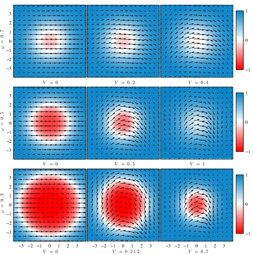
Figure 3: Computed droplet solutions for several choices of $\omega$ and $V$. The color contour plot represents the magnitude of $m_{3}$ and the arrows represent the projection of the magnetization on the plane. To facilitate visualization, the length of the projected field is normalized to the largest value in each frame.

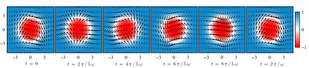
Figure 4: Precessional motion of a propagating droplet with $\omega=0.3$ and $V=0.212$ in the comoving frame. Each frame depicts a different instant in time over one period $2\pi/\omega$.

It is helpful to introduce the residual

$$r[f_{n}]=\mathcal{F}^{-1}\left[\widehat{Nf_{n}}-\left(\omega-V\kappa_{1}-\kappa^{2}\right)\widehat{f}\right],$$

which is zero at a droplet solution. We iterate from $f_{0}$ until

$$\|f_{n}-f_{n-1}\|_{\infty}<\mathrm{tol}_{f}\,,$$

$$\|r[f_{n}]\|_{\infty}<\mathrm{tol}_{r}\,,$$

$$|\tilde{\eta}_{n}-\tilde{\eta}_{n-1}|<\mathrm{tol}_{\eta}\,,$$

where we set $\mathrm{tol}_{f}=\mathrm{tol}_{\eta}=\mathrm{tol}_{r}=10^{-9}$, unless otherwise stated.

Further details and validation of this numerical scheme are presented in the Appendix.

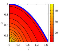
(a) Energy, $\mathcal{E}$

(b) Momentum, $\mathcal{P}_{1}$

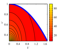
(c) Spin density, $\mathcal{N}$

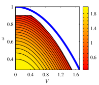
(d) Amplitude: $1-\min{(m_{3})}$

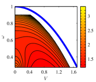
(e) Width ($x_{1}$-direction): $\mbox{width}_{1}$

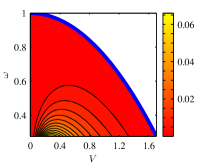
(f) Asymmetry ratio: $\frac{\mbox{width}_{2}-\mbox{width}_{1}}{\mbox{width}_{1}}$

Figure 5: Contour plots of the droplet’s energy, momentum, spin density, amplitude, width in the $x$-direction and asymmetry ratio, computed from numerical solutions of the boundary value problem.

5.2 Droplet Properties

Using the numerical scheme presented in the previous section, we computed a large number of solutions to the boundary value problem (37) for a propagating droplet with parameters lying in the set

$$\begin{split}S=\big{\{}(V,\omega)~{}|~{}&0\leq V\leq 2\sqrt{1-\omega}-0.25,\\ &0.275\leq\omega\leq 0.95\big{\}}.\end{split}$$

This representative set of droplet parameters was chosen because accurate solutions were obtained without having to change the numerical parameters of our scheme. Outside of this set, either higher resolution or larger domains were often required to accurately resolve the droplets (see Appendix). Droplets with $\omega<0$ were computed and exhibit similar properties to those in $S$. We were unable to compute large momentum droplets for particular $V$ with $\omega$ sufficiently small or negative due to inherently large phase gradients. Illustrative example droplet solutions are shown in Fig. 3. As $\omega$ and $V$ are increased, the droplet amplitude, defined as $1-\min{(m_{3})}=1-m_{3}(0,0)$, decreases. The spin wave background is evident, exhibiting a decreasing wavelength as $V$ is increased or as $\omega$ is decreased. This is in accord with the nonlinear dispersion relation discussed in Sec. 3.1. The precessional motion of a propagating droplet is depicted in Fig. 4 in the comoving frame.

Using Eq. (19), the energy $\mathcal{E}$, momentum $\mathcal{P}_{1}$, and spin density $\mathcal{N}$ were computed over $S$. Contour plots of these quantities are shown in Figs. 5(a)-5(c). Additional values of the conserved quantities outside $S$ were obtained by interpolation using the weakly nonlinear asymptotics (46). Both the energy and the spin density are monotone decreasing functions of $V$ and $\omega$. On the contrary, Fig. 5(b) shows that the momentum dependence is not monotonic. For fixed values of $\omega$, the momentum $\mathcal{P}_{1}$ exhibits a maximum for $V>0$. This “ridgeline” is shown as the dashed curve in Fig. 5(b). The droplets with the largest momentum exhibit the largest phase gradient near the origin. See, for example, the case $V=0.212$, $\omega=0.3$ in Figs. 3 and 4 which is on the ridgeline of large momentum droplets.

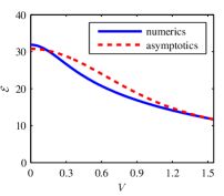
(a) Energy, $\mathcal{E}$

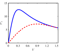
(b) Momentum, $\mathcal{P}_{1}$

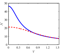
(c) Spin density, $\mathcal{N}$

Figure 6: Comparison of the weakly nonlinear asymptotics (46) with numerical computation of $\mathcal{E}$, $\mathcal{P}$, and $\mathcal{N}$ for $\omega=0.4$, $V_{\textrm{max}}\approx 1.55$.

Figure 6 depicts the numerical verification of the weakly nonlinear results (46) for fixed $\omega=0.4$. The results agree near the band edge where $V_{\textrm{max}}-V\ll 1$ and we have verified that the error exhibits the expected $\nu^{4}$ scaling.

The droplet’s amplitude dependence is shown in Fig. 5(d). As observed earlier, larger amplitude droplets correspond to smaller speeds and rest frequencies.

The droplets shown in Figs. 3 and 4 show negligible signs of asymmetry in their localization extent. To further investigate this, we define the droplet widths in the $x_{1}$ and $x_{2}$ directions according to the standard deviations

$$\mbox{width}_{1}= {\left(\frac{1}{\mathcal{N}}\,\int\,x_{1}^{2}\,\left(1-\cos{\Theta}\right)\,\mathrm{d}\vec{x}\right)}^{\frac{1}{2}}\,,$$ (57a)

$$\mbox{width}_{2}= {\left(\frac{1}{\mathcal{N}}\,\int\,x_{2}^{2}\,\left(1-\cos{\Theta}\right)\,\mathrm{d}\vec{x}\right)}^{\frac{1}{2}}\,.$$ (57b)

A contour plot of the quantity $\mbox{width}_{1}$ for $(V,\omega)\in S$ is shown in Fig. 5(e), exhibiting non monotonic behavior for increasing $V$ and $\omega$, especially for large amplitude modes. The droplet’s width diverges according to $\mathcal{O}(1/\nu(V,\omega))$ as the linear spin wave band is approached $0<\nu\ll 1$ (see Eq. (44)).

The asymmetry, defined as $(\mbox{width}_{2}-\mbox{width}_{1})/\mbox{width}_{1}$, is a nonnegative quantity as shown in Fig. 5(f). Even though the asymmetry does increase – approximately with the momentum – it is very small for droplets with parameters in $S$, reaching a maximum of approximately 0.066. Wide, small amplitude droplets are symmetric as shown in Eq. (44).

We now comment briefly on the localized excitations of Equation (10) observed in [10]. These states were formed by starting with a stationary droplet initial condition $f_{0}(\rho;\omega)=\sin\Theta_{0}(\rho;\omega)/[1+\cos\Theta_{0}(\rho;\omega)]$ to Eq. (18) superimposed with a spatially varying phase in the form

$$w(\vec{x},t=0)=e^{i\pi\vec{k}\cdot\vec{x}}f_{0}(|\vec{x}|;\omega).$$ (58)

This initial condition to Eq. (18) was allowed to evolve in time and a moving, localized structure was observed. The frequency of precession $\omega$, speed $V$, and energy $\mathcal{E}^{\prime}$ associated with several initial conditions reported in [10] are given in Table 1. For comparison, the energies $\mathcal{E}$ of directly computed propagating droplets with the same frequency and speed are also listed in Table 1. The droplet approximation (58) leads to overestimated energies which are less accurate for larger speeds. This behavior coincides with the small $V$ asymptotics of Sec. 4.2 which show that the ansatz in Eq. (58) is approximately valid.

$V$	$\omega$	$\mathcal{E}^{\prime}$	$\mathcal{E}$
0.067	0.50	25.6	25.5
0.13	0.49	25.9	25.8
0.24	0.47	27.0	26.9
0.3	0.46	28.9	27.8
0.35	0.44	31.4	28.8

Table 1: Comparison between the energies $\mathcal{E}^{\prime}$ computed in [10] by solving the initial value problem (58) with the energies $\mathcal{E}$ of droplets computed in this work.

5.3 Propagating Droplet Stability

The nonlinear, orbital stability of droplets has been supported by verification of the Jacobian condition (24) in the stationary [7] and weakly nonlinear [11] (recall Eq. (47)) cases. In this section, we confirm the stability of large amplitude, propagating droplets by numerically demonstrating that $J<0$ and by performing time-dependent numerical simulations of the LL Equation (10) with initially perturbed propagating droplets.

Figure 7 exhibits the numerical evaluation of the negative Jacobian $-J$ (33) for $(V,\omega)\in S$. Since $J<0$, we have numerically confirmed the invertibility of the map $(\omega,V)\mapsto(\mathcal{N},\mathcal{P}_{1})$ and the Jacobian condition (34) for droplet stability. The invertibility of the map is not obvious given the lack of monotonicity of $\mathcal{P}_{1}$ in Fig. 5(b). Note also that the Jacobian is monotonic in both $\omega$ and $V$ within the set $S$ and in the weakly nonlinear regime (Eq. (47)).

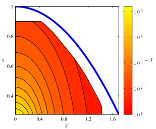
Figure 7: Numerical computation of the negative Jacobian $-J$ in Eq. (33) demonstrating that the map $(\omega,V)\mapsto(\mathcal{N},\mathcal{P}_{1})$ is invertible ($J\neq 0$) and the Jacobian condition $J<0$ for stability is satisfied.

Recalling that the Jacobian condition $J<0$ for orbital stability of solitary waves has only been demonstrated in other nonlinear wave systems [25, 22, 26], we seek further evidence of stability by performing time-dependent numerical simulations of perturbed droplets. To solve Eq. (10) numerically, we use the method of lines with a pseudospectral, Fourier discretization in space, the same as that used in our iterative numerical scheme of Sec. 5.1. For time stepping, we used an adaptive time stepping, second order Runge-Kutta ODE solver. Numerical parameters we used were $L=50$, $N=768$, giving $\Delta\approx 0.13$. Because the time stepping method does not preserve the length of the magnetization vector, after each time step the solution is rescaled so that $|\vec{m}|\equiv 1$ is preserved. The initial conditions consist of a computed droplet perturbed by noise (explained below). In all computations, we have verified that the quantities (11), (12), and (13) change at most by $0.74\%$ over the course of the simulation.

The initial conditions are constructed as follows. Uncorrelated, mean zero, normal random variables with variance 0.2 are sampled at each grid point to construct a complex valued noise function $n$. A low pass filter is applied with cutoff wavenumber 6 yielding $\tilde{n}$. Adding a droplet, $f$, computed as in Sec. 5.1 to the noise yields the perturbed droplet $\tilde{f}=f+\tilde{n}$ in stereographic form. Inverting the relation (17)

$$m_{3}=\frac{1-|\tilde{f}|^{2}}{1+|\tilde{f}|^{2}}\,,\quad m_{1}+im_{2}=(1+m_{3})\tilde{f}\,,$$

yields the initial condition for the LL equation (10) in vector form.

An example solution at $t=50$ is shown in Fig. 8. The perturbed droplet’s localization structure has been maintained. Furthermore, it’s propagation speed and precessional coherence have also been approximately maintained. To demonstrate this, we show in Figs. 9(a) and 9(b) the position and phase, respectively, of the minimum of the computed solution as a function of time. For comparison, we have included the trajectories of these quantities for unperturbed droplets. Stability for the considered droplets is clearly achieved with only small changes in the propagation speed and rest frequency.

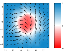
Figure 8: Perturbed droplet with $(V,\omega)=(0.7,0.3)$ at $t=50$. Compare with unperturbed case in Fig. 3.

These results suggest that droplets are robust, approximately maintaining their precessional frequency and propagation speed, even after experiencing significant perturbations.

The droplet iterative scheme of Sec. 5.1 converges for parameter values satisfying $\nu^{2}(V,\omega)<0$. However, as expected, such solutions are unstable due to linear spin wave resonances.

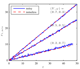
(a) $x_{1}$ position of solution minimum.

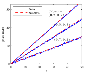
(b) Phase at solution minimum.

Figure 9: Time evolution of the $x_{1}$ position (a) and the phase (b) at the minimum of three perturbed droplets (solid curves) compared with unperturbed droplet evolution (dashed lines).

6 Discussion

In many respects, the 2D propagating nontopological droplet considered here has much in common with the 1D propagating droplet soliton reviewed in Sec. 3.2. Moreover, by rewriting Eqs. (26) in polar coordinates, it is immediate to observe that, for large values of the polar radius $\rho$, the droplet behaves as a 1-dimensional object (namely, depending only on $\rho$, with the velocity $V$ replaced by $V\,\cos{\varphi}$).

One interesting feature of the 1D case is the development of topological structure, a phase singularity for $V=0$ and $\omega<0$. While it is not possible for a single, topological solitary wave to stably propagate [18], the copropagation of pairs with opposite charge are possible [27]. The bifurcation of nontopological droplet solitary waves to pairs of topological structures have been predicted in isotropic ferromagnets [9] and in 2D, uniaxial, easy-plane ferromagnets [27]. It is natural to ask whether there exist propagating solutions with some local topological structure for the LL equation (10). Time-dependent numerical simulations of an appropriately chosen initial value problem have apparently yielded such structures [10]. Our computations with the stereographic Eq. (37) are limited to nonsingular, hence locally nontopological solutions. Furthermore, the large momentum states we have computed exhibit large phase gradients near the droplet center, suggesting the possibility of a bifurcation into local topological structure for sufficiently small or negative rest frequencies.

Another, necessarily multidimensional property of droplets was studied in [10] where ninety degree scattering was numerically observed for the head-on collision of two “accelerated” stationary droplets with the same frequency and opposite velocities. Merging accompanied by spin wave radiation was also observed for certain initial configurations. The propagating droplets constructed in this work could be used as initial conditions for a direct study of 2D droplet interactions.

7 Conclusions

Through numerical and asymptotic means, we have demonstrated the existence and studied the properties of moving droplets across a wide range of precessional frequencies and speeds as well as their stability to perturbations. Along with the rise of nanomagnetism research and applications [5], this work encourages further study of localized magnetic structures including droplet propagation in the presence of damping, external magnetic fields, nonlocal dipolar fields, and injected spin current.

Appendix: Validation of the Numerical Scheme

We validate the numerical scheme described in Sec. 5.1 in several ways. First, the Derrick identity (35) was checked for the computed droplet modes with $(V,\omega)\in S$. The largest deviation from zero of the quantity $d^{\prime}(1)$ in (35) was found to be approximately $5.3\cdot 10^{-8}$, which occurred for the stationary droplet $V=0$, $\omega=0.9$, likely due to the finite domain size.

Second, we verify that the resolution of the employed discretization is sufficiently fine to resolve the solution’s features. As can be observed in Fig. 10, we confirm that the relative magnitudes of the Fourier coefficients decay to machine precision for a large momentum droplet solution with $V=0.212$ and $\omega=0.3$. We find that all droplets with $(V,\omega)\in S$ show similar behavior with a large momentum droplet exhibiting the slowest decay to at most $4.9\cdot 10^{-9}$ for large $\kappa$, still an acceptable value. This suggests negligible aliasing effects so that we have properly resolved the solution.

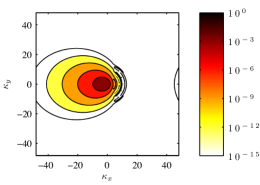
Figure 10: Absolute value of the Fourier coefficients, normalized by the maximum, for a single droplet with $\omega=0.3$ and $V=0.212$.

Finally, to determine a domain size and grid resolution that accurately resolves the droplets, we computed a very accurate, yardstick solution, $f_{\mathrm{ys}}$, with $V=0.7$ and $\omega=0.3$. The numerical parameters used were $L=50$, $N=2048$, $c=10$, and $\mathrm{tol}_{f}=\mathrm{tol}_{r}=\mathrm{tol}_{\eta}=10^{-13}$ so that $\Delta\approx 0.0488$. We compare $f_{\mathrm{ys}}$ with the same droplet mode obtained on different grids $(\Delta,L)$. The relative error $\|f_{\mathrm{ys}}-f\|_{\infty}/\|f_{\mathrm{ys}}\|_{\infty}$ is computed using sinc interpolation [35] of the yardstick to the grid for $f$ and plotted in Fig. 11. Domain truncation error decreases with increasing domain size until discretization error dominates. The smallest grid spacing $\Delta=0.075$ with $L>40$ yields relative errors below the precision of the yardstick tolerances. The iterative computations of droplets with $(V,\omega)\in S$ employ the conservative values $(\Delta,L)=(0.065,50)$, accounting for the larger phase gradients that occur.

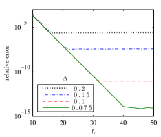
Figure 11: Relative error of the solution of the boundary value problem as a function of the domain size ($L_{1}=L_{2}=L$) for different values of the grid spacing ($\Delta_{1}=\Delta_{2}=\Delta$) for a single droplet with $\omega=0.3$ and $V=0.7$.

References

- [1] J. Slonczewski, Current-driven excitation of magnetic multilayers, J. Magn. Magn. Mater. 159 (1996) L1–L7.
- [2] M. Tsoi, A. G. M. Jansen, J. Bass, W. Chiang, M. Seck, V. Tsoi, P. Wyder, Excitation of a magnetic multilayer by an electric current, Phys. Rev. Lett. 80 (1998) 4281.
- [3] W. Rippard, M. Pufall, S. Kaka, S. Russek, T. Silva, Direct-Current induced dynamics in , Phys. Rev. Lett. 92 (2) (2004) 027201.
- [4] T. Silva, W. Rippard, Developments in nano-oscillators based upon spin-transfer point-contact devices, J. Magn. Magn. Mater. 320 (7) (2008) 1260–1271.
- [5] J. Lau, J. Shaw, Magnetic nanostructures for advanced technologies: fabrication, metrology and challenges, J. Phys. D: Appl. Phys. 44 (2011) 303001.
- [6] B. Ivanov, A. Kosevich, Bound-States of a large number of magnons in a ferromagnet with one-ion anisotropy, Zh. Exp. Teor. Fiz. 72 (5) (1977) 2000–2015.
- [7] A. Kosevich, B. Ivanov, A. Kovalev, Magnetic solitons, Phys. Rep. 194 (3-4) (1990) 117–238.
- [8] M. Hoefer, T. Silva, M. Keller, Theory for a dissipative droplet soliton excited by a spin torque nanocontact, Phys. Rev. B 82 (5) (2010) 054432.
- [9] N. Cooper, Solitary waves of planar ferromagnets and the breakdown of the spin-polarized quantum hall effect, Phys. Rev. Lett. 80 (20) (1998) 4554.
- [10] B. Piette, W. Zakrzewski, Localized solutions in a two-dimensional Landau-Lifshitz model, Physica D 119 (3-4) (1998) 314–326.
- [11] B. A. Ivanov, C. E. Zaspel, I. A. Yastremsky, Small-amplitude mobile solitons in the two-dimensional ferromagnet, Phys. Rev. B 63 (2001) 134413.
- [12] K. Long, A. Bishop, Nonlinear excitations in classical ferromagnetic chains, J. Phys. A: Math. Gen. 12 (8) (1979) 1325.
- [13] L. Landau, E. Lifshitz, Theory of the dispersion of magnetic permeability in ferromagnetic bodies, Phys. Z. Sowjet. 8 (1935) 153.
- [14] R. Kohn, V. Slastikov, Effective dynamics for ferromagnetic thin films: a rigorous justification, Proc. Roy. Soc. A 461 (2005) 143–154.
- [15] A. DeSimone, R. Kohn, S. Mueller, F. Otto, Recent analytical developments in micromagnetics, in G. Bertotti, I. Mayergoyz, eds., The Science of Hysteresis II: Physical Modeling, Micromagnetics, and Magnetization Dynamics, Elsevier, Amsterdam (2006) 269–381.
- [16] C. Melcher, Thin-film limits for Landau–Lifshitz–Gilbert equations, SIAM J. Math. Anal. 42 (2010) 519–537.
- [17] C. García-Cervera, One-dimensional magnetic domain walls, Eur. J. Appl. Math. 15 (2004) 451-486.
- [18] N. Papanicolaou, T. Tomaras, Dynamics of magnetic vortices, Nucl. Phys. B 360 (2-3) (1991) 425–462.
- [19] M. Lakshmanan, K. Nakamura, Landau-Lifshitz equation of ferromagnetism: Exact treatment of the Gilbert damping, Phys. Rev. Lett. 53 (1984) 2497.
- [20] C. Pethick, H. Smith, Bose-Einstein Condensation in Dilute Gases, Cambridge University Press, Cambridge, UK, (2002).
- [21] S. Gustafson, J. Shatah, The stability of localized solutions of Landau-Lifshitz equations, Comm. Pure Appl. Math. 55 (9) (2002) 1136–1159.
- [22] B. Ivanov, A. Sukstanskii, Three-dimensional solitons in ferrites and their stability, Sol. St. Comm. 50 (6) (1984) 523–527.
- [23] M. Vakhitov, A. Kolokolov, Stationary solutions of the wave equation in a medium with nonlinearity saturation, Radiophys. Quant. Elec. 16 (1973) 783–789.
- [24] T. Ioannidou, P. Sutcliffe, Soliton dynamics in 3D ferromagnets, Physica D 150 (1-2) (2001) 118–126.
- [25] I. Bar’yakhtar, B. Ivanov, Vector field dynamic solitons, Phys. Lett. A 98 (5-6) (1983) 222–226.
- [26] A. V. Buryak, Y. S. Kivshar, S. Trillo, Stability of three-wave parameteric solitons in diffractive quadratic media, Phys. Rev. Lett. 77 (1996) 5210.
- [27] N. Papanicolaou, P. Spathis, Semitopological solitons in planar ferromagnets, Nonlinearity 12 (1999) 285.
- [28] G. Derrick, Comments on nonlinear wave equations as models for elementary particles, J. Math. Phys. 5 (1964) 1252–1254.
- [29] S. Pohozaev, Eigenfunctions of the equation , Sov. Math. Dokl. 6 (1965) 1408–1411.
- [30] Z. Chen, N. Huang, Z. Liu, An inverse scattering transform for the Landau-Lifschitz equation for a spin chain with an easy axis, J. Phys.: Condens. Matter 7 (1995) 4533–4547.
- [31] R. Chiao, E. Garmire, C. Townes, Trapping of optical beams, Phys. Rev. Lett 13 (1964) 479–482.
- [32] C. Sulem, P. Sulem, The nonlinear Schrödinger equation, Springer, New York, 1999.
- [33] M. Ablowitz, Z. Musslimani, Spectral renormalization method for computing self-localized solutions to nonlinear systems, Opt. Lett. 30 (2005) 2140–2142.
- [34] V. Petviashvili, Equation of an extraordinary soliton, Sov. J. Plasma Phys. 2 (1976) 469.
- [35] F. Stenger, Summary of sinc numerical methods, J. Comp. Appl. Math. 121 (1-2) (2000) 379–420.