Numerical Solutions of Optimal Risk Control and Dividend Optimization Policies under A Generalized Singular Control Formulation

Abstract

This paper develops numerical methods for finding optimal dividend pay-out and reinsurance policies. A generalized singular control formulation of surplus and discounted payoff function are introduced, where the surplus is modeled by a regime-switching process subject to both regular and singular controls. To approximate the value function and optimal controls, Markov chain approximation techniques are used to construct a discrete-time controlled Markov chain with two components. The proofs of the convergence of the approximation sequence to the surplus process and the value function are given. Examples of proportional and excess-of-loss reinsurance are presented to illustrate the applicability of the numerical methods.

Key Words. Singular control, dividend policy, Markov chain approximation, numerical method, reinsurance, regime switching.

1 Introduction

To design optimal risk controls and and dividend payout strategies for a financial corporation has drawn increasing attention since the introduction of the classical collective risk model in Lundberg, (1903), where the probability of ruin was considered as a measure of risk. Realizing that the surplus reaching arbitrarily high and exceeding any finite level are not realistic in practice, De Finetti, (1957) proposed an dividend optimization problem. Instead of considering the safety aspect (ruin probability), aiming at maximizing the expected discounted total dividends until lifetime ruin by assuming the surplus process follows a simple random walk, he showed that the optimal dividend strategy is a barrier strategy. Since then, many researchers have analyzed this problem under more realistic assumptions and extended its range of applications. Some recent work can be found in Asmussen and Taksar, (1997); Choulli et al., (2001); Gerber and Shiu, (2004) and references therein. To protect insurance companies against the impact of claim volatilities, reinsurance is a standard tool with the goal of reducing and eliminating risk. The primary insurance carrier pays the reinsurance company a certain part of the premiums. In return, the reinsurance company is obliged to share the risk of large claims. Proportional reinsurance is one type of reinsurance policy. Within this scheme, the reinsurance company covers a fixed percentage of losses. The other type of reinsurance policy is nonproportional reinsurance. The most common nonproportional reinsurance policy is the so-called excess-of-loss reinsurance, within which the cedent (primary insurance carrier) will pay all of the claims up to a pre-given level of amount (termed retention level). The comparison of these two types of reinsurance can be found in Asmusen et al., (2000). In this paper, we consider both of these reinsurance policies and provide the numerical solutions of the corresponding Markovian regime-switching models.

Let $u(t)$ be an exogenous retention level, which is a control chosen by the insurance company representing the reinsurance policy. In a Cremér-Lundberg model, claims arrive according a Poisson process with rate $\beta$. Let $Y_{i}$ be the size of the $i$th claim. The $Y_{i}$’s are independent and identically distributed (i.i.d.) random variables. Let $Y_{i}^{u}$ be the the fraction of the claims hold by the cedent. The insurer selects the time and the amount of dividends to be paid out to the policyholders. Let $X(t)$ denote the controlled surplus of an insurance company at time $t\geq 0$. Throughout this paper, we only consider cheap reinsurance, where the safety loading for the reinsurer is the same as that for the cedent. The numerical scheme and the convergence proofs are also applicable to more general reinsurance problems. By using the techniques of diffusion approximation applied to the Cremér-Lundberg model, the surplus process satisfies

$$\begin{cases}dX(t)=\beta E[Y_{i}^{u}]dt+\sqrt{\beta E[(Y_{i}^{u})^{2}])}dw(t),\\ X(0^{-})=x,\end{cases}$$ (1.1)

where $w(t)$ is a standard Brownian motion. In the case of proportional reinsurance, $Y_{i}^{u}=uY_{i}$. Thus, following (1.1), the surplus is given by

$$\begin{cases}dX(t)=\beta u(t)E[Y_{i}]dt+u(t)\sqrt{\beta E[Y_{i}^{2}]}dw(t),\\ X(0^{-})=x,\end{cases}$$ (1.2)

In the case of excess-of-loss reinsurance, $Y_{i}^{u}=Y_{i}\wedge u$ with the retention level $u$. We have

$$\begin{array}[]{ll}&\!\!\!\displaystyle E[Y^{u}]=\int_{0}^{u}\bar{F}(x)dx,\ E[(Y^{u})^{2}]=\int_{0}^{u}2x\bar{F}(x)dx\end{array}$$ (1.3)

where $\bar{F}(x)=P(Y_{i}>x)$. The stochastic differential equation of the surplus process follows

$$\left\{\begin{array}[]{ll}&\!\!\!\displaystyle dX(t)=\beta\int_{0}^{u(t)}\bar{F}(x)dxdt+\Big{[}\beta\int_{0}^{u(t)}\bar{F}(x)dx\Big{]}^{\frac{1}{2}}dw(t),\\ &\!\!\!\displaystyle X(0^{-})=x.\end{array}\right.$$ (1.4)

A common choice of the payoff is to maximize the total expected discounted value of all dividends until lifetime ruin; see Gerber and Shiu, (2006) and Jin et al., (2011). Let

$$\tau:=\inf\left\{t>0:X(t)\notin G\right\}$$ (1.5)

be the ruin time, where $G=(0,\infty)$ is the domain of the surplus. Denote by $r>0$ the discounting factor, and by $Z(t)$ the total dividends paid out up to time $t$. Our goal is to maximize

$$E\int_{0}^{\tau}e^{-rt}dZ(t).$$ (1.6)

Some “bequest” functions and more complicated utility functions are added to the payoff functions in the work Browne, (1995, 1997). In this paper, we treat payoff functions that are more general and complex than those given in (1.6) or Browne, (1995, 1997); our proposed numerical methods are easily implementable.

A dividend strategy $Z(\cdot)$ is an ${\cal F}_{t}$-adapted process $\{Z(t):t\geq 0\}$ corresponding to the accumulated amount of dividends paid up to time $t$ such that $Z(t)$ is a nonnegative and nondecreasing stochastic process that is right continuous with left limits. Throughout the paper, we use the convention that $Z(0^{-})=0$. In general, a dividend process is not necessarily absolutely continuous. In fact, dividends are not usually paid out continuously in practice. For instance, insurance companies may distribute dividends on discrete time intervals resulting in unbounded payment rate. In such a scenario, the surplus level changes drastically on a dividend payday. Thus abrupt or discontinuous changes occur due to “singular” dividend distribution policy. Together with proportional or excess-of-loss reinsurance policy, this gives rise to a mixed regular-singular stochastic control problem.

Empirical studies indicate in particular that traditional surplus models fail to capture more extreme price movements. To better reflect reality, much effort has been devoted to producing better models. One of the recent trends is to use regime-switching models. Hamilton, (1989) introduced a regime-switching time series model. Recent work on risk models and related issues can be found in Asmussen, (1989); Yang and Yin, (2004). In Wei et al., (2010), the optimal dividend and proportional reinsurance strategy under utility criteria were studied for the regime-switching compound Poisson model by using the methods of the classical and impulse control theory. Sotomayor and Cadenillas, (2011) obtained optimal dividend strategies under a regime-switching diffusion model. A comprehensive study of switching diffusions with “state-dependent” switching is in Yin and Zhu, (2010).

In this work, we model the surplus process by a regime-switching diffusion; reinsurance and dividend payment policies are introduced as regular and singular stochastic controls. The goal is to maximize the expected total discounted payoff until ruin; see (2.2) for details. The model we consider appears to be more versatile and realistic than the classical compound Poisson or diffusion models. To find the optimal reinsurance and dividend pay-out strategies, one usually solves a so-called Hamilton-Jacobi-Bellman (HJB) equation. However, in our work, thanks to regime switching and the mixed regular and singular control formulation, the HJB equation is in fact a coupled system of nonlinear quasi-variational inequalities (QVIs). A closed-form solution is virtually impossible to obtain. A viable alternative is to employ numerical approximations. In this work, we adapt the Markov chain approximation methodology developed by Kushner and Dupuis, (2001). To the best of our knowledge, numerical methods for singular controls of regime-switching diffusions have not been studied in the literature to date. Even for singular controlled diffusions without regime switching, the related results are relatively scarce; Budhiraja and Ross, (2007) and Kushner and Martins, (1991) are the only papers that carry out a convergence analysis using weak convergence and relaxed control formulation of numerical schemes for singular control problems in the setting of Itô diffusions. We focus on developing numerical methods that are applicable to mixed regular and singular controls for regime-switching models. Although the primary motivation stems from insurance risk controls, the techniques and the algorithms suggested appear to be applicable to other singular control problems. It is also worth mentioning that the Markov chain approximation method requires little regularity of the value function and/or analytic properties of the associated systems of HJB equations and/or QVIs. The numerical implementation can be done using either value iterations or policy iterations.

The rest of the paper is organized as follows. A generalized formulation of optimal risk control and dividend policies and assumptions are presented in Section 2. The two most common types of reinsurance strategy (proportional reinsurance and excess-of-loss reinsurance) are covered in our study. Section 3 deals with the numerical algorithm of Markov chain approximation method. The regular control and the singular control are well approximated by the approximating Markov chain and the dynamic programming equation are presented. Section 4 deals with the convergence of the approximation scheme. The technique of “rescaling time” is introduced and the convergence theorems are proved. Two classes of numerical examples are provided in Section 5 to illustrate the performance of the approximation method. Finally, some additional remarks are provided in Section 6.

2 Formulation

In this section, we introduce a dynamic system to describe the surplus processes with reinsurance and dividend payout strategies with Markov regime switching. Let $X(t)$ denote the controlled surplus of an insurance company at time $t\geq 0$. Denote by $u(t)$ and $Z(t)$ the dynamic reinsurance policy at time $t$ and the total dividend paid out up to time $t$, respectively. Assume the evolution of $X(t)$, subject to reinsurance and dividend payments, follows a one-dimensional temporal homogeneous controlled regime-switching diffusion on an unbounded domain $G=(0,\infty)$:

$$\begin{cases}dX(t)=b(X(t),\alpha(t),u(t))dt+\sigma(X(t),\alpha(t),u(t))dW(t)-dZ(t),\\ X(0^{-})=x\in G,\ \ \alpha(0^{-})=\ell\in{\cal M},\end{cases}$$ (2.1)

where $u$ is the regular control and $Z$ is the singular control. Throughout the paper we use the convention that $Z(0^{-})=0$. The jump size of $Z$ at time $t\geq 0$ is denoted by $\Delta Z(t):=Z(t)-Z(t^{-})$, and $Z^{c}(t):=Z(t)-\sum_{0\leq s\leq t}\Delta Z(s)$ denotes the continuous part of $Z$. Also note that $\Delta X(t):=X(t)-X(t^{-})=-\Delta Z(t)$ for any $t\geq 0$.

Denote by $r>0$ the discounting factor. For suitable functions $f$ and $c$ and an arbitrary admissible pair $\pi=(u,Z)$, the expected discounted payoff is

$$J(x,\ell,\pi)=E_{x,\ell}\left[\int_{0}^{\tau}e^{-rt}\left[f(X(t),\alpha(t),u(t))dt+c(X(t^{-}),\alpha(t^{-}))dZ(t)\right]\right].$$ (2.2)

The pair $\pi=(u,Z)$ is said to be admissible if $u$ and $Z$ satisfy

• $u(t)$ and $Z(t)$ are nonnegative for any $t\geq 0$,

• $Z$ is càdlàg and nondecreasing,

• $X(t)\geq 0$, for any $t\leq\tau$, where $\tau$ is the ruin time defined in (1.5),

• both $u$ and $Z$ are adapted to ${\cal F}_{t}:=\sigma\left\{W(s),\alpha(s),0\leq s\leq t\right\}$ augmented by the ${P}$-null sets, and

• $J(x,\ell,\pi)<\infty$ for any $(x,\ell)\in G\times{\cal M}$ and admissible pair $\pi=(u,Z)$, where $J$ is the functional defined in (2.2).

Suppose that $\mathcal{A}$ is the collection of all admissible pairs, and $U$ is the collection of possible retention levels $u(t)$. Throughout the paper, we assume that $U$ is a given compact set, and that for each $\ell\in{\cal M}$, $c(x,\ell)\geq c(y,\ell)$ for all $0\leq x\leq y$. That is, the utility function for the dividend is non-decreasing, see examples in Gerber and Shiu, (2005) and Alvarez, (2000). In addition, $c(X(t),\ell)=f(X(t),\ell,u)=0$ when $t>\tau$. Define the value function as

$$V(x,\ell):=\sup_{\pi\in\cal A}J(x,\ell,\pi).$$ (2.3)

If the value function $V$ defined in (2.3) is sufficiently smooth, by applying the dynamic programming principle (Fleming and Soner, (2006)), we conclude formerly that $V$ satisfies the following coupled system of quasi variational inequalities (QVIs):

$$\max\left\{H(x,\ell,V^{\prime}(x,\ell),V^{\prime\prime}(x,\ell))+Q(x)V(x,\cdot)(\ell)-rV(x,\ell),c(x,\ell)-V^{\prime}(x,\ell)\right\}=0,$$ (2.4)

for all $(t,x,\ell)\in[0,\tau)\times G\times{\cal M},$ with boundary condition

$$V(0,\ell)=0,\ \ \forall\ell\in{\cal M},$$ (2.5)

where for any $(x,\ell,p)\in\times{\mathbb{R}}^{n}\times{\cal M}\times{\mathbb{R}}^{n}$,

$$\begin{array}[]{rl}&\!\!\!\displaystyle H(x,\ell,p):=\sup_{u\in U}\big{\{}f(x,\ell,u)+p\cdot b(x,\ell,u)+\frac{1}{2}\sigma^{2}(x,\ell,u)\big{\}},\\ &\!\!\!\displaystyle Q(x)V(x,\cdot)(\ell):=\sum_{\iota\in{\cal M}}q_{\ell\iota}(x)[V(x,\iota)-V(x,\ell)],\end{array}$$

and $V^{\prime}$ and $V^{\prime\prime}$ denote the first and the second partial derivatives of $V$ with respect to $x$. Note that coupling in (2.4) is due to the term $Q(x)V(t,x,\cdot)(\ell)$, which is not contained in the usual QVI (as in Fleming and Soner, (2006); Ma and Yong, (1999); Pham, (2009)).

Nevertheless, the value function $V$ is not necessarily smooth. In fact, there are examples (Bayraktar et al., (2011)) where the value function is not even continuous. In our work, both the ruin time $\tau$ and the reinsurance $u$ and the dividend $Z$ policies may depend on the initial surplus level, which leads to nonsmooth vale function. Moreover, (2.4) is a coupled system of nonlinear differential equations. A closed-form solution to (2.4) is by and large impossible. Therefore in this work, we propose a numerical scheme to approximate the value function as well as optimal reinsurance and dividend payment policies.

3 Numerical Algorithm

Our goal is to design a numerical scheme to approximate value function $V$ in (2.3). As a standing assumption, we assume $V(\cdot)$ is continuous with respect to $x$. In this section we construct a locally consistent Markov chain approximation for the mixed regular-singular control model with regime-switching. The discrete-time and finite-state controlled Markov chain is so defined that it is locally consistent with (2.1). Note that the state of the process has two components $x$ and $\alpha$. Hence in order to use the methodology in Kushner and Dupuis, (2001), our approximating Markov chain must have two components: one component delineates the diffusive behavior whereas the other keeps track of the regimes. Let $h>0$ be a discretization parameter. Define $L_{h}=\{x:x=kh,k=0,\pm 1,\pm 2,\dots\}$ and $S_{h}=L_{h}\cap G_{h}$, where $G_{h}=(0,B+h)$ and $B$ is an upper bound introduced for numerical computation purpose. Moreover, assume without loss of generality that the boundary point $B$ is an integer multiple of $h$. Let $\{(\xi_{n}^{h},\alpha_{n}^{h}),n<\infty\}$ be a controlled discrete-time Markov chain on $S_{h}\times{\cal M}$ and denote by $p^{h}((x,\ell),(y,\iota)|\pi^{h})$ the transition probability from a state $(x,\ell)$ to another state $(y,\iota)$ under the control $\pi^{h}$. We need to define $p^{h}$ so that the chain’s evolution well approximates the local behavior of the controlled regime-switching diffusion (2.1). At any discrete time $n$, we can either exercise a regular control, a singular control or a reflection step. That is, if we put $\Delta\xi_{n}^{h}=\xi_{n+1}^{h}-\xi_{n}^{h}$, then

$$\Delta\xi_{n}^{h}=\Delta\xi_{n}^{h}I_{\left\{\text{regular control step at }n\right\}}+\Delta\xi_{n}^{h}I_{\left\{\text{singular control step at }n\right\}}+\Delta\xi_{n}^{h}I_{\left\{\text{reflection step at }n\right\}}.$$ (3.1)

The chain and the control will be chosen so that there is exactly one term in (3.1) is nonzero. Denote by $\left\{I_{n}^{h}:n=0,1,\dots\right\}$ a sequence of control actions, where $I_{n}^{h}=0,1$ or $2$, if we exercise a singular control, regular control, or reflection at time $n$, respectively.

If $I_{n}^{h}=1$, then we denote by $u_{n}^{h}\subset U$ the random variable that is the regular control action for the chain at time $n$. Let $\tilde{\Delta}t^{h}(\cdot,\cdot,\cdot)>0$ be the interpolation interval on $S_{h}\times{\cal M}\times U$. Assume $\inf_{x,\ell,u}\tilde{\Delta}t^{h}(x,\ell,u)>0$ for each $h>0$ and $\lim_{h\to 0}\sup_{x,\ell,u}\tilde{\Delta}t^{h}(x,\ell,u)\to 0$.

Let $E_{x,\ell,n}^{u,h,1}$, ${\text{Var}}_{x,\ell,n}^{u,h,1}$ and ${P}_{x,\ell,n}^{u,h,1}$ denote the conditional expectation, variance, and marginal probability given $\{\xi_{k}^{h},\alpha_{k}^{h},u_{k}^{h},I_{k}^{h},k\leq n,\xi_{n}^{h}=x,\alpha_{n}^{h}=\ell,I_{n}^{h}=1,u_{n}^{h}=u\}$, respectively. The sequence $\{(\xi_{n}^{h},\alpha_{n}^{h})\}$ is said to be locally consistent, if it satisfies

$$\begin{array}[]{ll}&\!\!\!\displaystyle E_{x,\ell,n}^{u,h,1}[\Delta\xi_{n}^{h}]=b(x,\ell,u)\tilde{\Delta}t^{h}(x,\ell,u)+o(\tilde{\Delta}t^{h}(x,\ell,u)),\\[6.45831pt] &\!\!\!\displaystyle\text{Var}_{x,\ell,n}^{u,h,1}(\Delta\xi_{n}^{h})=\sigma^{2}(x,\ell,u)\tilde{\Delta}t^{h}(x,\ell,u)+o(\tilde{\Delta}t^{h}(x,\ell,u)),\\[6.45831pt] &\!\!\!\displaystyle{P}_{x,\ell,n}^{u,h,1}\{\alpha_{n+1}^{h}=\iota\}=q_{\ell\iota}(x)\tilde{\Delta}t^{h}(x,\ell,u)+o(\tilde{\Delta}t^{h}(x,\ell,u)),\text{ for }\iota\neq\ell,\\[6.45831pt] &\!\!\!\displaystyle{P}_{x,\ell,n}^{u,h,1}\{\alpha_{n+1}^{h}=\ell\}=(1+q_{\ell\ell}(x))\tilde{\Delta}t^{h}(x,\ell,u)+o(\tilde{\Delta}t^{h}(x,\ell,u)).\\[6.45831pt] &\!\!\!\displaystyle\sup_{n,\omega\in\Omega}|\Delta\xi_{n}^{h}|\to 0\ \hbox{ as }\ h\to 0.\end{array}$$

If $I_{n}^{h}=0$, then we denote by $\Delta z_{n}^{h}$ the random variable that is the singular control action for the chain at time $n$ if $\xi_{n}^{h}\in[0,B]$. Note that $\Delta\xi_{n}^{h}=-\Delta z_{n}^{h}=-h$. If $I_{n}^{h}=2$, or $\xi_{n}^{h}=B+h$, reflection step is exerted definitely. Dividend is paid out to lower the surplus level. Moreover, we require reflection takes the state from $B+h$ to $B$. That is, if we denote by $\Delta g_{n}^{h}$ the random variable that is the reflection action for the chain at time $n$, then $\Delta\xi_{n}^{h}=-\Delta g_{n}^{h}=-h$.

The singular control can be seen as a combination of “inside” part ($I_{n}^{h}=0$) and “boundary” part ($I_{n}^{h}=2$). Also we require the singular control and reflection to be “impulsive” or “instantaneous.” In other words, the interpolation interval on $S_{h}\times{\cal M}\times U\times\left\{0,1,2\right\}$ is

$$\Delta t^{h}(x,\ell,u,i)=\tilde{\Delta}t^{h}(x,\ell,u)I_{\left\{i=1\right\}},\text{ for any }(x,\ell,u,i)\in S_{h}\times{\cal M}\times U\times\left\{0,1,2\right\}.$$ (3.2)

Denote by $\pi^{h}:=\{\pi_{n}^{h},n\geq 0\}$ the sequence of control actions, where

$$\pi_{n}^{h}:=\Delta z^{h}_{n}I_{\{I_{n}^{h}=0\}}+u_{n}^{h}I_{\{I_{n}^{h}=1\}}+\Delta g^{h}_{n}I_{\{I_{n}^{h}=2\}}.$$

The sequence $\pi^{h}$ is said to be admissible if $\pi_{n}^{h}$ is $\sigma\left\{(\xi_{0}^{h},\alpha_{0}^{h}),\dots,(\xi_{n}^{h},\alpha_{n}^{h}),\pi_{0}^{h},\dots,\pi^{h}_{n-1}\right\}$-adapted and for any $E\in\mathcal{B}(S_{h}\times{\cal M})$, we have

$${P}\left\{(\xi_{n+1}^{h},\alpha_{n+1}^{h})\in E\big{|}\sigma\{(\xi_{0}^{h},\alpha_{0}^{h}),\dots,(\xi_{n}^{h},\alpha_{n}^{h}),\pi_{0}^{h},\dots,\pi^{h}_{n}\}\right\}=p^{h}((\xi_{n}^{h},\alpha_{n}^{h}),E|\pi_{n}^{h}),$$

and

$${P}\left\{(\xi_{n+1}^{h},\alpha^{h}_{n+1})=(B,\ell)\big{|}(\xi_{n}^{h},\alpha_{n}^{h})=(B+h,\ell),\sigma\{(\xi_{0}^{h},\alpha_{0}^{h}),\dots,(\xi_{n}^{h},\alpha_{n}^{h}),\pi_{0}^{h},\dots,\pi^{h}_{n}\}\right\}=1.$$

Put

$$t_{0}^{h}:=0,\ t_{n}^{h}:=\sum_{k=0}^{n-1}\Delta t^{h}(\xi_{k}^{h},\alpha_{k}^{h},u_{k}^{h},I_{k}^{h}),\ \text{ and }n^{h}(t):=\max\left\{n:t_{n}^{h}\leq t\right\}.$$

Then the piecewise constant interpolations, denoted by $(\xi^{h}(\cdot),\alpha^{h}(\cdot))$, $u^{h}(\cdot)$, $g^{h}(\cdot)$, and $z^{h}(\cdot)$, are naturally defined as

$$\xi^{h}(t)=\xi_{n}^{h},\ \alpha^{h}(t)=\alpha_{n}^{h},\ u^{h}(t)=u_{n}^{h},\ g^{h}(t)=\sum_{k\leq n^{h}(t)}\Delta g_{k}^{h}I_{\left\{I_{k}^{h}=2\right\}},\ z^{h}(t)=\sum_{k\leq n^{h}(t)}\Delta z_{k}^{h}I_{\left\{I_{k}^{h}=0\right\}},$$ (3.3)

for $t\in[t_{n}^{h},t_{n+1}^{h})$. Let $\eta_{h}:=\inf\left\{n:\xi_{n}^{h}\in\partial G\right\}$. Then the first exit time of $\xi^{h}$ from $G$ is $\tau^{h}=t^{h}_{\eta_{h}}$. Let $(\xi_{0}^{h},\alpha_{0}^{h})=(x,\ell)\in S_{h}\times{\cal M}$ and $\pi^{h}$ be an admissible control. The cost function for the controlled Markov chain is defined as

$$J_{B}^{h}(x,\ell,\pi^{h})=E\sum_{k=1}^{\eta_{h}-1}e^{-rt_{k}^{h}}[f(\xi_{k}^{h},\alpha_{k}^{h},u_{k}^{h})\Delta t_{k}^{h}+c(\xi_{k}^{h},\alpha_{k}^{h})\Delta z_{k}^{h}],$$ (3.4)

which is analogous to (2.2) thanks to the definition of interpolation intervals in (3.2). The value function of the controlled Markov chain is

$$V^{h}_{B}(x,\ell)=\displaystyle\sup_{\pi^{h}\text{ admissible}}J^{h}_{B}(x,\ell,\pi^{h}).$$ (3.5)

We shall show that $V^{h}_{B}(x,\ell)$ satisfies the dynamic programming equation:

$$V^{h}_{B}(x,\ell)=\left\{\begin{array}[]{ll}&\!\!\!\displaystyle\displaystyle\max_{u\in U}\bigg{\{}\sum_{(y,\iota)}e^{-r\Delta t^{h}(x,\ell,u,1)}p^{h}((x,\ell),(y,\iota)|\pi)V^{h}(y,\iota)+f(x,\ell,u)\Delta t^{h}(x,\ell,u,1),\\ &\displaystyle\qquad\qquad\big{[}\displaystyle\sum_{(y,\iota)}p^{h}((x,\ell),(y,\iota)|\pi)V^{h}(y,\iota)+c(x,\ell)h\big{]}\bigg{\}},\ \ \text{ for }x\in S_{h},\\ &\displaystyle 0,\ \hfill\text{ for }x=0.\end{array}\right.$$ (3.6)

Note that discounting does not appear in the second line above because singular control is impulsive. In the actual computing, we use iteration in value space or iteration in policy space together with Gauss-Seidel iteration to solve $V^{h}$. The computations will be very involved. In contrast to the usual state space $S_{h}$ in Kushner and Dupuis, (2001), here we need to deal with an enlarged state space $S_{h}\times{\cal M}$ due to the presence of regime switching.

Define the approximation to the first and the second derivatives of $V(\cdot,\ell)$ by finite difference method in the first part of QVIs (2.4) using stepsize $h>0$ as:

$$\begin{array}[]{ll}&\!\!\!\displaystyle V(x,\ell)\to V^{h}(x,\ell)\\ &\!\!\!\displaystyle V_{x}(x,\ell)\to\frac{V^{h}(x+h,\ell)-V^{h}(x,\ell)}{h}\ \hbox{ for }\ b(x,\ell,u)>0,\\ &\!\!\!\displaystyle V_{x}(x,\ell)\to\frac{V^{h}(x,\ell)-V^{h}(x-h,\ell)}{h}\ \hbox{ for }\ b(x,\ell,u)<0,\\ &\!\!\!\displaystyle V_{xx}(x,\ell)\to\frac{V^{h}(x+h,\ell)-2V^{h}(x,\ell)+V^{h}(x-h,\ell)}{h^{2}}.\end{array}$$ (3.7)

For the second part of the QVIs, we choose

$$V_{x}(x,\ell)\to\frac{V^{h}(x,\ell)-V^{h}(x-h,\ell)}{h}.$$

Together with the boundary conditions, it leads to

$$\begin{array}[]{ll}&\!\!\!\displaystyle V^{h}(x,\ell)=0,\ \hbox{for}\ x=0,\\ &\!\!\!\displaystyle\max_{u\in U}\Big{\{}\frac{V^{h}(x+h,\ell)-V^{h}(x,\ell)}{h}b(x,\ell,u)^{+}-\frac{V^{h}(x,\ell)-V^{h}(x-h,\ell)}{h}b(x,\ell,u)^{-}\\ &\displaystyle\ \ +\frac{V^{h}(x+h,\ell)-2V^{h}(x,\ell)+V^{h}(x-h,\ell)}{h^{2}}\frac{\sigma^{2}(x,\ell,u)}{2}\\ &\displaystyle\ \ +\sum_{\iota}V^{h}(x,\cdot)q_{\ell\iota}-rV^{h}(x,\ell)+u,\ \ \ c(x,\ell)-\frac{V^{h}(x,\ell)-V^{h}(x-h,\ell)}{h}\Big{\}}=0,\\ &\displaystyle\qquad\qquad\forall x\in G_{h}^{o},\ell\in\cal{M},\end{array}$$ (3.8)

where $b(x,\ell,u)^{+}$ and $b(x,\ell,u)^{-}$ are the positive and negative parts of $b(x,\ell,u)$, respectively. Simplifying (3.8) and comparing the result with (3.6), we achieve the transition probabilities of the first part of the right side of (3.6) as the following:

$$\begin{array}[]{ll}&\!\!\!\displaystyle p^{h}((x,\ell),(x+h,\ell)|\pi)=\frac{(\sigma^{2}(x,\ell,u)/2)+hb(x,\ell,u)^{+}}{D-rh^{2}},\\ &\!\!\!\displaystyle p^{h}((x,\ell),(x-h,\ell)|\pi)=\frac{(\sigma^{2}(x,\ell,u)/2)+hb(x,\ell,u)^{-}}{D-rh^{2}},\\ &\!\!\!\displaystyle p^{h}((x,\ell),(x,\iota)|\pi)=\frac{h^{2}}{D-rh^{2}}q_{\ell\iota},\ \ \hbox{for}\ \ \ell\neq\iota,\\ &\!\!\!\displaystyle p^{h}(\cdot)=0,\ \ \hbox{otherwise},\\ &\!\!\!\displaystyle\Delta t^{h}(x,\ell,u,1)=\frac{h^{2}}{D},\end{array}$$ (3.9)

with

$$D=\sigma^{2}(x,\ell,u)+h|b(x,\ell,u)|+h^{2}(r-q_{\ell\ell})$$

being well defined. We also find the transition probability for the second part of the right side of (3.6). That is,

$$p^{h}((x,\ell),(x-h,\ell)|\pi)=1.$$

Remark 3.1.

The transition probabilities are quite natural. The first part of the QVIs can be seen as a “diffusion” region, where the regular control is dominant. The Markov approximating chain can switch between regimes and states nearby. But the second part of the QVIs is the “jump” region, where the dividends are paid out and the singular control is dominant. The singular control will project the Markov approximation chain back one step $h$ w.p.1 due to the representation.

Since the wealth can not reach infinity, we need only need choose $B$ large enough and compute the value function in the finite interval $[0,B]$. Our ultimate goal is to show $V^{h}$ converges to $V$ in a large enough interval $[0,B]$ as $h\to 0$. A common approach (Kushner and Dupuis, (2001)) is to show that the collection $\left\{(\xi^{h},\alpha^{h}),u^{h},g^{h},z^{h},h\geq 0\right\}$ is tight and then appropriately characterize the subsequential weak limit. However, the above scheme is problematic since in general, the processes $\left\{g^{h}(\cdot),z^{h}(\cdot),h\geq 0\right\}$ may fail to be tight. To overcome this difficulty, we adapt the techniques developed in Kushner and Martins, (1991) and Budhiraja and Ross, (2007). The basic idea is to (a) suitably re-scale the time so that the processes involved in the convergence analysis are tight in the new time scale; (b) carry out weak convergence analysis with the rescaled processes; and (c) revert back to the original time scale to obtain the convergence of $V^{h}$ to $V$. Note that the setting in our problem is different from those in the aforementioned references. Moreover, the presence of regime switching adds additional difficulty in the analysis.

4 Convergence of Numerical Approximation

This section focuses on the asymptotic properties of the approximating Markov chain proposed in the last section. The main techniques are methods of weak convergence. To begin with, the technique of time rescaling is given in Section 4.1. The interpolation of the approximation sequences is introduced in Section 4.1. The definition of relax controls and chattering lemmas of optimal control are presented in Sections 4.2 and 4.3, respectively. Section 4.4 deals with weak convergence of $\{\hat{\xi}^{h}(\cdot),\hat{\alpha}^{h}(\cdot),\hat{m}^{h}(\cdot),\hat{w}^{h}(\cdot),\hat{z}^{h}(\cdot),\hat{g}^{h}(\cdot),\hat{T}^{h}(\cdot)\}$, a sequence of rescaled process. As a result, a sequence of controlled surplus processes converges to a limit surplus process. By using the techniques of inversion, Section 4.4 also takes up the issue of the weak convergence of the surplus process. Finally Section 4.5 establishes the convergence of the value function.

4.1 Interpolation and Rescaling

Based on the approximating Markov chain constructed above, the piecewise constant interpolation is obtained and the appropriate interpolation interval level is chosen. Recalling (3.3), the continuous-time interpolations $(\xi^{h}(\cdot),\alpha^{h}(\cdot))$, $u^{h}(\cdot)$, $g^{h}(\cdot)$, and $z^{h}(\cdot)$ are defined. In addition, let ${\cal{U}}^{h}$ denote the collection of controls, which are determined by a sequence of measurable functions $F_{n}^{h}(\cdot)$ such that

$$u_{n}^{h}=F_{n}^{h}(\xi_{k}^{h},\alpha_{k}^{h},k\leq n;u_{k}^{h},k\leq n).$$ (4.1)

Define ${\cal{D}}_{t}^{h}$ as the smallest $\sigma$-algebra generated by $\{\xi^{h}(s),\alpha^{h}(s),u^{h}(s),g^{h}(s),z^{h}(s),$ $s\leq t\}.$ In addition, $\cal{U}$^h defined by (4.1) is equivalent to the collection of all piecewise constant admissible controls with respect to $\cal{D}$${}_{t}^{h}.$

Using the representations of regular control, singular control, reflection step and the interpolations defined above, (3.1) yields

$$\begin{array}[]{ll}\xi^{h}(t)&\!\!\!\displaystyle=x+\sum_{k=0}^{n-1}[E_{k}^{h}\Delta\xi_{k}^{h}+(\Delta\xi_{k}^{h}-E_{k}^{h}\Delta\xi_{k}^{h})]-z^{h}(t)-g^{h}(t)\\ &\!\!\!\displaystyle=x+\sum_{k=0}^{n-1}b(\xi_{k}^{h},\alpha_{k}^{h},u_{k}^{h})\Delta t^{h}(\xi_{k}^{h},\alpha_{k}^{h},u_{k}^{h})+\sum_{k=0}^{n-1}(\Delta\xi_{k}^{h}-E_{k}^{h}\Delta\xi_{k}^{h})-z^{h}(t)-g^{h}(t)+\varepsilon^{h}(t)\\ &\!\!\!\displaystyle=x+B^{h}(t)+M^{h}(t)-z^{h}(t)-g^{h}(t)+\varepsilon^{h}(t),\end{array}$$ (4.2)

where

$$B^{h}(t)=\sum_{k=0}^{n-1}b(\xi_{k}^{h},\alpha_{k}^{h},u_{k}^{h})\Delta t^{h}(\xi_{k}^{h},\alpha_{k}^{h},u_{k}^{h}),$$

$$M^{h}(t)=\sum_{k=0}^{n-1}(\Delta\xi_{k}^{h}-E_{k}^{h}\Delta\xi_{k}^{h}),$$

and $\varepsilon^{h}(t)$ is a negligible error satisfying

$$\lim_{h\to\infty}\sup_{0\leq t\leq T}E|\varepsilon^{h}(t)|^{2}\to 0\ \hbox{ for any }\ 0<T<\infty.$$ (4.3)

Also, $M^{h}(t)$ is a martingale with respect to $\cal{D}$${}_{t}^{h}$, and its discontinuity goes to zero as $h\to 0.$ We attempt to represent $M^{h}(t)$ in a form similar to the diffusion term in (2.1). Define $w^{h}(\cdot)$ as

$$\begin{array}[]{ll}w^{h}(t)&\!\!\!\displaystyle=\sum_{k=0}^{n-1}(\Delta\xi_{k}^{h}-E_{k}^{h}\Delta\xi_{k}^{h})/\sigma(\xi_{k}^{h},\alpha_{k}^{h},u_{k}^{h}),\\ &\!\!\!\displaystyle=\int_{0}^{t}\sigma^{-1}(\xi^{h}(s),\alpha^{h}(s),u^{h}(s))dM^{h}(s).\end{array}$$ (4.4)

We can now rewrite (4.2) as

$$\xi^{h}(t)=x+\int_{0}^{t}b(\xi^{h}(s),\alpha^{h}(s),u^{h}(s))ds+\int_{0}^{t}\sigma(\xi^{h}(s),\alpha^{h}(s),u^{h}(s))dw^{h}(s)-z^{h}(t)-g^{h}(t)+\varepsilon^{h}(t).$$ (4.5)

Next we will introduce the rescaling process. The basic idea of rescaling time is to “stretch out” the control and state processes so that they are “smoother” and therefore the tightness of $g^{h}(\cdot)$ and $z^{h}(\cdot)$ can be proved. Define $\Delta\hat{t}_{n}^{h}$ by

$$\Delta\hat{t}_{n}^{h}=\begin{cases}\Delta t^{h}\ \ \ \hbox{ for a diffusion on step $n$},\\ |\Delta z_{n}^{h}|=h\ \ \ \hbox{ for a singular control on step $n$},\\ |\Delta g_{n}^{h}|=h\ \ \ \hbox{ for a reflection on step $n$},\end{cases}$$ (4.6)

Define $\hat{T}^{h}(\cdot)$ by

$$\hat{T}^{h}(t)=\sum_{i=0}^{n-1}\Delta t^{h}=t_{n}^{h},\ \ \ \hbox{for}\ \ t\in[\hat{t}_{n}^{h},\hat{t}_{n+1}^{h}]$$

Thus, $\hat{T}^{h}(\cdot)$ will increase with the slope of unity if an only if a regular control is exerted. In addition, define the rescaled and interpolated process $\hat{\xi}^{h}(t)=\xi^{h}(\hat{T}^{h}(t))$, likewise define $\hat{\alpha}^{h}(t))$, $\hat{u}^{h}(t)$, $\hat{g}^{h}(t)$ similarly. The time scale is stretched out by $h$ at the reflection and singular control steps. We can now write

$$\hat{\xi}^{h}(t)=x +\int_{0}^{t}b(\hat{\xi}^{h}(s),\hat{\alpha}^{h}(s),\hat{u}^{h}(s))ds$$ (4.7)

$$+\int_{0}^{t}\sigma(\hat{\xi}^{h}(s),\hat{\alpha}^{h}(s),\hat{u}^{h}(s))dw^{h}(s)-\hat{z}^{h}(t)-\hat{g}^{h}(t)+\varepsilon^{h}(t).$$

4.2 Relaxed Controls

Let ${\cal B}({U}\times[0,\infty))$ be the $\sigma$-algebra of Borel subsets of ${U}\times[0,\infty)$. An admissible relaxed control (or deterministic relaxed control) $m(\cdot)$ is a measure on ${\cal B}({U}\times[0,\infty))$ such that $m({U}\times[0,t])=t$ for each $t\geq 0$. Given a relaxed control $m(\cdot)$, there is an $m_{t}(\cdot)$ such that $m(d\phi dt)=m_{t}(d\phi)dt$. We can define $m_{t}(B)=\lim_{\delta\to 0}{\frac{m(B\times[t-\delta,t])}{\delta}}$ for $B\in{\cal B}(U)$. With the given probability space, we say that $m(\cdot)$ is an admissible relaxed (stochastic) control for $(w(\cdot),\alpha(\cdot))$ or $(m(\cdot),w(\cdot),\alpha(\cdot))$ is admissible, if $m(\cdot,\omega)$ is a deterministic relaxed control with probability one and if $m(A\times[0,t])$ is ${\cal F}_{t}$-adapted for all $A\in{\cal B}(U)$. There is a derivative $m_{t}(\cdot)$ such that $m_{t}(\cdot)$ is ${\cal F}_{t}$-adapted for all $A\in{\cal B}(U)$.

Given a relaxed control $m(\cdot)$ of $u^{h}(\cdot)$, we define the derivative $m_{t}(\cdot)$ such that

$$m^{h}(K)=\int_{U\times[0,\infty)}I_{\{(u^{h},t)\in K\}}m_{t}(d\phi)dt$$ (4.8)

for all $K\in{\cal B}(U\times[0,\infty))$, and that for each $t,$ $m_{t}(\cdot)$ is a measure on ${\cal B}(U)$ satisfying $m_{t}(U)=1$. For example, we can define $m_{t}(\cdot)$ in any convenient way for $t=0$ and as the left-hand derivative for $t>0$,

$$m_{t}(A)=\lim_{\delta\to 0}\frac{m(A\times[t-\delta,t])}{\delta},\ \forall A\in{\mathcal{B}}(U).$$ (4.9)

Note that $m(d\phi dt)=m_{t}(d\phi)dt$. It is natural to define the relaxed control representation $m^{h}(\cdot)$ of $u^{h}(\cdot)$ by

$$m_{t}^{h}(A)=I_{\{u^{h}(t)\in A\}},\ \forall A\in{\mathcal{B}}(U).$$ (4.10)

Let ${\cal F}_{t}^{h}$ be a filtration, which denotes the minimal $\sigma$-algebra that measures

$$\{\xi^{h}(s),\alpha^{h}(\cdot),m_{s}^{h}(\cdot),w^{h}(s),z^{h}(s),g^{h}(s),s\leq t\}.$$ (4.11)

Use ${\Gamma}^{h}$ to denote the set of admissible relaxed controls $m^{h}(\cdot)$ with respect to $(\alpha^{h}(\cdot),w^{h}(\cdot))$ such that $m_{t}^{h}(\cdot)$ is a fixed probability measure in the interval $[t_{n}^{h},t_{n+1}^{h})$ given ${\cal F}_{t}^{h}$. Then $\Gamma^{h}$ is a larger control space containing ${\cal U}^{h}$. Referring to the stretched out time scale, we denote the rescaled relax control as $m_{\hat{T}^{h}(t)}(d\phi)$. Define $M_{t}(A)$ and $M^{h}_{t}(d\phi)$ by

$$\begin{array}[]{ll}&\!\!\!\displaystyle M_{t}(A)dt=dw(t)I_{u(t)\in A},\ \forall A\in{\mathcal{B}}(U)\\ &\!\!\!\displaystyle M^{h}_{t}(d\phi)dt=dw^{h}(t)I_{u^{h}(t)\in\cal U}.\end{array}$$

Analogously, as an extension of time rescaling, we let

$$\hat{M}^{h}_{\hat{T}^{h}(t)}(d\phi)d\hat{T}^{h}(t)=d\hat{w}^{h}(\hat{T}^{h}(t))I_{u^{h}(\hat{T}^{h}(t))\in\cal U}.$$

With the notation of relaxed control given above, we can write (4.5), (4.7) and the value function (2.3) as

$$\xi^{h}(t)=x+\int_{0}^{t}\int_{\cal U}b(\xi^{h}(s),\alpha^{h}(s),\phi)m_{s}^{h}(d\phi)ds+\int_{0}^{t}\int_{\cal U}\sigma(\xi^{h}(s),\alpha^{h}(s),\phi)M^{h}_{s}(d\phi)ds+\varepsilon^{h}(t),$$ (4.12)

$$\begin{array}[]{ll}\hat{\xi}^{h}(t)=&\!\!\!\displaystyle x+\int_{0}^{t}\int_{\cal U}b(\hat{\xi}^{h}(s),\hat{\alpha}^{h}(s),\phi)\hat{m}_{\hat{T}^{h}(s)}^{h}(d\phi)d\hat{T}^{h}(s)\\ &\displaystyle\hfill+\int_{0}^{t}\int_{\cal U}\sigma(\hat{\xi}^{h}(s),\hat{\alpha}^{h}(s),\phi)\hat{M}_{\hat{T}^{h}(s)}(d\phi)d\hat{T}^{h}(s)-\hat{z}^{h}(t)-\hat{g}^{h}(t)+\varepsilon^{h}(t),\end{array}$$ (4.13)

and

$$V^{h}(x,\ell)=\inf_{m^{h}\in\Gamma^{h}}J^{h}(x,\ell,m^{h}).$$ (4.14)

Now we give the definition of existence and uniqueness of weak solution.

Definition 4.1.

By a weak solution of (4.12), we mean that there exists a probability space $(\Omega,{\cal F},P)$, a filtration ${\cal F}_{t}$, and process $(x(\cdot),\alpha(\cdot),m(\cdot),w(\cdot))$ such that $w(\cdot)$ is a standard ${\cal F}_{t}$-Wiener process, $\alpha(\cdot)$ is a Markov chain with generator $Q$ and state space ${\cal M}$, $m(\cdot)$ is admissible with respect to $x(\cdot)$, and is ${\cal F}_{t}$-adapted, and (4.12) is satisfied. For an initial condition $(x,\ell)$, by the weak sense uniqueness, we mean that the probability law of the admissible process $(\alpha(\cdot),m(\cdot),w(\cdot))$ determines the probability law of solution $(x(\cdot),\alpha(\cdot),m(\cdot),w(\cdot))$ to (4.12), irrespective of probability space.

To proceed, we need some assumptions.

• Let $u(\cdot)$ be an admissible ordinary control with respect to $w(\cdot)$ and $\alpha(\cdot)$, and suppose that $u(\cdot)$ is piecewise constant and takes only a finite number of values. For each initial condition, there exists a solution to (4.12) where $m(\cdot)$ is the relaxed control representation of $u(\cdot)$. This solution is unique in the weak sense.

4.3 A Chattering Lemma and Approximation to the Optimal Control

This section deals with the approximation of relaxed controls by ordinary controls. We can always use relax controls to approximate the ordinary controls, which is only a tool for mathematical analysis. Here we present a result of chattering lemma for our problem. The proof of the chattering lemma can be found in Kushner, (1990).

Proposition 4.2.

Let $(m(\cdot),w(\cdot))$ be admissible for the problem given in (4.12). Then given $\varsigma>0$, there is a finite set $\{\gamma^{\varsigma}_{1},\ldots,\gamma^{\varsigma}_{l_{\varsigma}}\}=U^{\varsigma}\subset U$, and an $\varepsilon>0$ such that there is a probability space on which are defined $(x^{\varsigma}(\cdot),\alpha^{\varsigma}(\cdot),u^{\varsigma}(\cdot),w^{\varsigma}(\cdot))$, where $w^{\varsigma}(\cdot)$ are standard Brownian motions, and $u^{\varsigma}(\cdot)$ is an admissible $U^{\varsigma}$-valued ordinary control on the interval $[k\varepsilon,k\varepsilon+\varepsilon)$. Moreover,

$$\begin{array}[]{ll}&\!\!\!\displaystyle P^{m}_{x}\left(\sup_{s\leq T}|x^{\varsigma}(s)-x(s)|>\varsigma\right)\leq\varsigma,\ and\\ &\!\!\!\displaystyle|J^{m}_{x}(\cdot)-J^{u^{\varsigma}}_{x}(\cdot)|\leq\varsigma.\end{array}$$ (4.15)

Coming back to the approximation to the optimal control, to show that the discrete approximation of the value function $V^{h}(x,\ell)$ converges to the value function $V(x,\ell)$, we shall use the comparison control techniques. In doing so, we need to verify certain continuity properties. The details of the proof is presented in the appendix.

Proposition 4.3.

For (4.12), let $\widetilde{\varsigma}>0$ be given and $(x(\cdot),\alpha(\cdot),m(\cdot),w(\cdot))$ be an $\widetilde{\varsigma}$-optimal control. For each $\varsigma>0$, there is an $\varepsilon>0$ and a probability space on which are defined $w^{\varsigma}(\cdot)$, a control $u^{\varsigma}(\cdot)$ as in Theorem 4.2, and a solution $x^{\varsigma}(\cdot)$ such that the following assertions hold:

• $$|J^{m}_{x}(\cdot)-J^{u^{\varsigma}}_{x}(\cdot)|\leq\varsigma.$$ (4.16)

• Moreover, there is a $\theta>0$ such that the approximating $u^{\varsigma}(\cdot)$ can be chosen so that its probability law at $n\varepsilon$, conditioned on $\{w^{\varsigma}(\tau),\alpha^{\varsigma}(\tau),\tau\leq n\varepsilon;u^{\varsigma}(k\varepsilon),k<n\}$ depends only on the samples $\{w^{\varsigma}(p\theta),\alpha^{\varsigma}(p\theta),p\theta\leq n\varepsilon;u^{\varsigma}(k\varepsilon),k<n\}$, and is continuous in the $w^{\varepsilon}(p\theta)$ arguments.

4.4 Convergence of A Sequence of Surplus Processes

Lemma 4.4.

Using the transition probabilities $\{p^{h}(\cdot)\}$ defined in (3.9), the interpolated process of the constructed Markov chain $\{\hat{\alpha}^{h}(\cdot)\}$ converges weakly to $\hat{\alpha}(\cdot)$, the Markov chain with generator $Q=(q_{\ell\iota})$.

Proof. It can be seen that $\alpha^{h}(\cdot)$ is tight. The proof can be obtained similar to Theorem 3.1 in Yin et al., (2003). That is,

$$\left|E[(\alpha^{h}(t+s)-\alpha^{h}(t))^{2}]|{\cal F}_{t}^{h}\right|\leq\tilde{\gamma}(s)\ \ \hbox{and}\ \ \lim_{s\to 0}\lim_{h\to 0}\sup E\tilde{\gamma}(s)=0,$$ (4.17)

where $\tilde{\gamma}(s)\geq 0$ is ${\cal F}_{t}^{h}$-measurable. On the other hand, due to the definition of $\hat{\alpha}^{h}(\cdot)$, we have

$$\left|E[(\hat{\alpha}^{h}(t+s)-\hat{\alpha}^{h}(t))^{2}]|{\cal F}_{t}^{h}\right|\leq\left|E[(\alpha^{h}(t+s)-\alpha^{h}(t))^{2}]|{\cal F}_{t}^{h}\right|\leq\tilde{\gamma}(s).$$ (4.18)

Combining (4.17) and (4.18), we obtain $\hat{\alpha}^{h}(\cdot)$ is tight. Thus, the constructed Markov chain $\{\hat{\alpha}^{h}(\cdot)\}$ converges weakly to $\hat{\alpha}(\cdot)$. $\Box$

Theorem 4.5.

Let the approximating chain $\{\xi_{n}^{h},\alpha_{n}^{h},n<\infty\}$ constructed with transition probabilities defined in (3.9) be locally consistent with (2.1), $m^{h}(\cdot)$ be the relaxed control representation of $\{u_{n}^{h},n<\infty\}$, $(\xi^{h}(\cdot),\alpha^{h}(\cdot))$ be the continuous-time interpolation defined in (3.3), and $\{\hat{\xi}^{h}(\cdot),\hat{\alpha}^{h}(\cdot),\hat{m}^{h}(\cdot),\hat{w}^{h}(\cdot),\hat{z}^{h}(\cdot),\hat{g}^{h}(\cdot),\hat{T}^{h}(\cdot)\}$ be the corresponding rescaled processes. Then $\{\hat{\xi}^{h}(\cdot),\hat{\alpha}^{h}(\cdot),\hat{m}^{h}(\cdot),\hat{w}^{h}(\cdot),\hat{z}^{h}(\cdot),\hat{g}^{h}(\cdot),\hat{T}^{h}(\cdot)\}$ is tight.

Proof. In view of Lemma 4.4, $\{\hat{\alpha}^{h}(\cdot)\}$ is tight. The sequence $\{\hat{m}^{h}(\cdot)\}$ is tight since its range space is compact. Let $T<\infty$, and let $\tau_{h}$ be an ${\cal F}_{t}$-stopping time which is no bigger than $T$. Then for $\delta>0$,

$$E_{\tau_{h}}^{u^{h}}(w^{h}(\tau_{h}+\delta)-w^{h}(\tau_{h}))^{2}=\delta+{\varepsilon}_{h},$$ (4.19)

where ${\varepsilon}_{h}\to 0$ uniformly in $\tau_{h}$. Taking $\limsup_{h\to 0}$ followed by $\lim_{\delta\to 0}$ yield the tightness of $\{w^{h}(\cdot)\}$. Similar to the argument of $\alpha^{h}(\cdot)$, the tightness of $\hat{w}^{h}(\cdot)$ is obtained. Furthermore, following the definition of “stretched out” timescale,

$$\begin{array}[]{ll}&\!\!\!\displaystyle|\hat{z}^{h}(\tau_{h}+\delta)-\hat{z}^{h}(\tau_{h})|\leq|\delta|+O(h),\\ &\!\!\!\displaystyle|\hat{g}^{h}(\tau_{h}+\delta)-\hat{g}^{h}(\tau_{h})|\leq|\delta|+O(h).\end{array}$$

Thus $\{\hat{z}^{h}(\cdot),\hat{g}^{h}(\cdot)\}$ is tight. For notational simplicity, we assume that $b(\cdot)$ and $\sigma(\cdot)$ are bounded. For more general case, we can use a truncation device. These results and the boundedness of $b(\cdot)$ implies the tightness of $\{\xi^{h}(\cdot)\}$. Therefore it follows that

$$\{\hat{\xi}^{h}(\cdot),\hat{\alpha}^{h}(\cdot),\hat{u}^{h}(\cdot),\hat{w}^{h}(\cdot),\hat{z}^{h}(\cdot),\hat{g}^{h}(\cdot),\hat{T}^{h}(\cdot)\}$$

is tight. $\Box$

Since $\{\hat{x}^{h}(\cdot),\hat{\alpha}^{h}(\cdot),\hat{m}^{h}(\cdot),\hat{w}^{h}(\cdot),\hat{z}^{h}(\cdot),\hat{g}^{h}(\cdot),\hat{T}^{h}(\cdot)\}$ is tight, we can extract a weakly convergent subsequence denoted by $\{\hat{\xi}(\cdot),\hat{\alpha}(\cdot),\hat{m}(\cdot),\hat{w}(\cdot),\hat{z}(\cdot),\hat{g}(\cdot),\hat{T}(\cdot)\}$. Also, the paths of $\{\hat{x}(\cdot),\hat{\alpha}(\cdot),\hat{m}(\cdot),\hat{w}(\cdot),\hat{z}(\cdot),\hat{g}(\cdot),\hat{T}(\cdot)\}$ are continuous w.p.1.

Theorem 4.6.

Let $\{\hat{x}(\cdot),\hat{\alpha}(\cdot),\hat{m}(\cdot),\hat{w}(\cdot),\hat{z}(\cdot),\hat{g}(\cdot),\hat{T}(\cdot)\}$ be the limit of weakly convergent subsequence of $\{\hat{\xi}^{h}(\cdot),\hat{\alpha}^{h}(\cdot),\hat{m}^{h}(\cdot),\hat{w}^{h}(\cdot),\hat{z}^{h}(\cdot),\hat{g}^{h}(\cdot),\hat{T}^{h}(\cdot)\}$. $w(\cdot)$ is a standard ${\cal F}_{t}$-Wiener process, and $m(\cdot)$ is admissible. Let $\hat{\cal F}_{t}$ the $\sigma$-algebra generated by $\{\hat{\xi}^{h}(\cdot),\hat{\alpha}^{h}(\cdot),\hat{m}^{h}(\cdot),\hat{w}^{h}(\cdot),$ $\hat{z}^{h}(\cdot),\hat{g}^{h}(\cdot),\hat{T}^{h}(\cdot)\}$. Then $\hat{w}(t)=w(\hat{T}(t))$ is an $\hat{\cal F}_{t}$-martingale with quadratic variation $\hat{T}(t)$. The limit processes satisfy

$$\begin{array}[]{ll}\hat{x}(t)&\!\!\!\displaystyle=x+\int_{0}^{t}\int_{\cal U}b(\hat{x}(s),\hat{\alpha}(s),\phi)\hat{m}_{\hat{T}(s)}^{h}(d\phi)d\hat{T}(s)\\ &\displaystyle\ +\int_{0}^{t}\int_{\cal U}\sigma(\hat{x}(s),\hat{\alpha}(s),\phi)\hat{M}_{\hat{T}(s)}(d\phi)d\hat{T}(s)-\hat{z}(t)-\hat{g}(t).\end{array}$$ (4.20)

Proof. For $\delta>0$, define the process $l(\cdot)$ by $l^{h,\delta}(t)=l^{h}(n\delta),t\in[n\delta,(n+1)\delta)$. Then, by the tightness of $\{\hat{\xi}^{h}(\cdot),\hat{\alpha}^{h}(\cdot)\}$, (4.13) can be rewritten as

$$\begin{array}[]{ll}\hat{\xi}^{h}(t)&\!\!\!\displaystyle=x+\int_{0}^{t}\int_{\cal U}b(\hat{\xi}^{h}(s),\hat{\alpha}^{h}(s),\phi)\hat{m}_{\hat{T}^{h}(s)}^{h}(d\phi)d\hat{T}^{h}(s)\\ &\displaystyle\quad+\int_{0}^{t}\int_{\cal U}\sigma(\hat{\xi}^{h,\delta}(s),\hat{\alpha}^{h,\delta}(s),\phi)\hat{M}_{\hat{T}^{h}(s)}(d\phi)d\hat{T}^{h}(s)-\hat{z}^{h}(t)-\hat{g}^{h}(t)+\varepsilon^{h,\delta}(t),\end{array}$$ (4.21)

where

$$\lim_{\delta\to 0}\limsup_{h\to 0}E|\varepsilon^{h,\delta}(t)|=0.$$ (4.22)

If we can verify $\hat{w}(\cdot)$ to be an $\hat{\cal F}_{t}$-martingale, then (4.20) could be obtained by taking limits in (4.21). To characterize $w(\cdot)$, let $t>0,$ $\delta>0$, $p$, $q$, $\{t_{k}:k\leq p\}$ be given such that $t_{k}\leq t\leq t+s$ for all $k\leq p$, $\psi_{j}(\cdot)$ for $j\leq q$ is real-valued and continuous functions on $U\times[0,\infty)$ having compact support for all $j\leq q$. Define

$$(\psi_{j},\hat{m})_{t}=\int_{0}^{t}\int_{\cal U}\psi_{j}(\phi,s)\hat{m}_{\hat{T}(s)}^{h}(d\phi)d\hat{T}(s).$$ (4.23)

Let $S(\cdot)$ be a real-valued and continuous function of its arguments with compact support. By (4.4), $w^{h}(\cdot)$ is an ${\cal F}_{t}$-martingale. In view of the definition of $\hat{w}(t)$, we have

$$ES(\hat{\xi}^{h}(t_{k}),\hat{\alpha}^{h}(t_{k}),\hat{w}^{h}(t_{k}),(\psi_{j},m^{h})_{t_{k}},\hat{z}^{h}(t_{k}),\hat{g}^{h}(t_{k}),j\leq q,k\leq p)[\hat{w}^{h}(t+s)-\hat{w}^{h}(t)]=0.$$ (4.24)

By using the Skorohod representation and the dominant convergence theorem, letting $h\to 0,$ we obtain

$$ES(\hat{\xi}^{h}(t_{k}),\hat{\alpha}^{h}(t_{k}),\hat{w}^{h}(t_{k}),(\psi_{j},m^{h})_{t_{k}},\hat{z}^{h}(t_{k}),\hat{g}^{h}(t_{k}),j\leq q,k\leq p)[\hat{w}(t+s)-\hat{w}(t)]=0.$$ (4.25)

Since $\hat{w}(\cdot)$ has continuous sample paths, (4.25) implies that $\hat{w}(\cdot)$ is a continuous ${\cal F}_{t}$-martingale. On the other hand, since

$$E[((\hat{w}^{h}(t+\delta))^{2}-(\hat{w}^{h}(t))^{2}]=E[(\hat{w}^{h}(t+\delta)-\hat{w}^{h}(t))^{2}]=\hat{T}(t+s)-\hat{T}(t),$$ (4.26)

by using the Skorohod representation and the dominant convergence theorem together with (4.26), we have

$$\begin{array}[]{ll}&\!\!\!\displaystyle ES(\hat{\xi}^{h}(t_{k}),\hat{\alpha}^{h}(t_{k}),\hat{w}^{h}(t_{k}),(\psi_{j},m^{h})_{t_{k}},\hat{z}^{h}(t_{k}),\hat{g}^{h}(t_{k}),j\leq q,k\leq p)\\ &\displaystyle\hfill\times[\hat{w}^{2}(t+\delta)-\hat{w}^{2}(t)-(\hat{T}(t+s)-\hat{T}(t))]=0.\end{array}$$ (4.27)

The quadratic variation of the martingale $\hat{w}(t)$ is $\Delta\hat{T}$, then $\hat{w}(\cdot)$ is an $\hat{\cal F}_{t}$-Wiener process.

Let $h\to 0$, by using the Skorohod representation, we obtain

$$\begin{array}[]{ll}&\!\!\!\displaystyle E\left|\int_{0}^{t}\int_{\cal U}b(\hat{\xi}^{h}(s),\hat{\alpha}^{h}(s),\phi)\hat{m}_{\hat{T}^{h}(s)}^{h}(d\phi)d\hat{T}^{h}(s)-\int_{0}^{t}\int_{\cal U}b(\hat{x}(s),\hat{\alpha}(s),\phi)\hat{m}_{\hat{T}(s)}^{h}(d\phi)d\hat{T}(s)\right|=0\end{array}$$ (4.28)

uniformly in $t$ with probability one. On the other hand, $\{\hat{m}^{h}(\cdot)\}$ converges in the compact weak topology, that is, for any bounded and continuous function $\psi(\cdot)$ with compact support, as $h\to 0$,

$$\int_{0}^{\infty}\int_{\cal U}\psi(\phi,s)\hat{m}_{\hat{T}^{h}(s)}^{h}(d\phi)d\hat{T}^{h}(s)\to\int_{0}^{\infty}\int_{\cal U}\psi(\phi,s)\hat{m}_{\hat{T}(s)}(d\phi)d\hat{T}(s).$$ (4.29)

Again, the Skorohod representation (with a slight abuse of notation) implies that as $h\to 0$,

$$\begin{array}[]{ll}&\!\!\!\displaystyle\int_{0}^{t}\int_{\cal U}b(\hat{\xi}^{h}(s),\hat{\alpha}^{h}(s),\phi)\hat{m}_{\hat{T}^{h}(s)}^{h}(d\phi)d\hat{T}^{h}(s)\to\int_{0}^{t}\int_{\cal U}b(\hat{x}(s),\hat{\alpha}(s),\phi)\hat{m}_{\hat{T}(s)}(d\phi)d\hat{T}(s)\end{array}$$ (4.30)

uniformly in $t$ with probability one on any bounded interval.

In view of (4.21), since $\xi^{h,\delta}(\cdot)$ and $\alpha^{h,\delta}(\cdot)$ are piecewise constant functions,

$$\int_{0}^{t}\int_{\cal U}\sigma(\hat{\xi}^{h,\delta}(s),\hat{\alpha}^{h,\delta}(s),\phi)\hat{M}_{\hat{T}^{h}(s)}(d\phi)d\hat{T}^{h}(s)\to\int_{0}^{t}\int_{\cal U}\sigma(\hat{x}^{\delta}(s),\hat{\alpha}^{\delta}(s),\phi)\hat{M}_{\hat{T}(s)}(d\phi)d\hat{T}(s)$$ (4.31)

as $h\to 0$. Combining (4.23)-(4.31), we have

$$\begin{array}[]{ll}\hat{x}(t)&\!\!\!\displaystyle=x+\int_{0}^{t}\int_{\cal U}b(\hat{x}(s),\hat{\alpha}(s),\phi)\hat{m}_{\hat{T}(s)}^{h}(d\phi)d\hat{T}(s)\\ &\displaystyle\quad+\int_{0}^{t}\int_{\cal U}\sigma(\hat{x}^{\delta}(s),\hat{\alpha}^{\delta}(s),\phi)\hat{M}_{\hat{T}(s)}(d\phi)d\hat{T}(s)-\hat{z}(t)-\hat{g}(t)+\varepsilon^{\delta}(t),\end{array}$$ (4.32)

where $\lim_{\delta\to 0}E|\varepsilon^{\delta}(t)|=0.$ Finally, taking limits in the above equation as $\delta\to 0$, (4.20) is obtained. $\Box$

Theorem 4.7.

For $t<\infty$, define the inverse

$$R(t)=\inf\{s:\hat{T}(s)>t\}.$$

Then $R(t)$ is right continuous and $R(t)\to\infty$ as $t\to\infty$ w.p.1. For any process $\hat{\varphi}(\cdot)$, define the rescaled process $\varphi(\cdot)$ by $\varphi(t)=\hat{\varphi}(T(t))$. Then, $w(\cdot)$ is a standard ${\cal F}_{t}$-Wiener process and (2.1) holds.

Proof. Since $\hat{T}(t)\to\infty$ w.p.1 as $t\to\infty$, $R(t)$ exists for all $t$ and $R(t)\to\infty$ as $t\to\infty$ w.p.1. Similar to (4.25) and (4.27),

$$ES(\xi^{h}(t_{k}),\alpha^{h}(t_{k}),w^{h}(t_{k}),(\psi_{j},m^{h})_{t_{k}},z^{h}(t_{k}),g^{h}(t_{k}),j\leq q,k\leq p)\times[w(t+s)-w(t)]=0.$$

$$\begin{array}[]{ll}&\!\!\!\displaystyle ES(\xi^{h}(t_{k}),\alpha^{h}(t_{k}),w^{h}(t_{k}),(\psi_{j},m^{h})_{t_{k}},z^{h}(t_{k}),g^{h}(t_{k}),j\leq q,k\leq p)\\ &\displaystyle\hfill\times[w^{2}(t+\delta)-w^{2}(t)-(R(t+s)-R(t))]=0.\end{array}$$

Thus, we can verify $w(\cdot)$ is an ${\cal F}_{t}$-Wiener process. A rescaling of (4.20) yields

$$\begin{array}[]{ll}x(t)=x&\!\!\!\displaystyle+\int_{0}^{t}\int_{\cal U}b(x(s),\alpha(s),\phi)m_{s}(d\phi)ds\\ &\!\!\!\displaystyle+\int_{0}^{t}\int_{\cal U}\sigma(x(s),\alpha(s),\phi)M_{s}(d\phi)ds-z(t)-g(t).\end{array}$$ (4.33)

In other words, (2.1) holds. $\Box$

4.5 Convergence of Cost and Value Functions

Theorem 4.8.

Let $h$ index the weak convergent subsequence of $\{\hat{\xi}^{h}(\cdot),\hat{\alpha}^{h}(\cdot),\hat{m}^{h}(\cdot),\hat{w}^{h}(\cdot),\\ \hat{z}^{h}(\cdot),\hat{g}^{h}(\cdot),\hat{T}^{h}(\cdot)\}$ with the limit $\{\hat{x}(\cdot),\hat{\alpha}(\cdot),\hat{m}(\cdot),\hat{w}(\cdot),\hat{z}(\cdot),\hat{g}(\cdot),\hat{T}(\cdot)\}$. Then,

$$\begin{array}[]{ll}J^{h}(x,\ell,\pi^{h})&\!\!\!\displaystyle\to E_{x,\ell}^{\pi}\int_{0}^{\tau}\int_{\cal U}e^{-r\hat{T}(t)}[f(\hat{x}(t),\hat{\alpha}(t),\phi)\hat{m}_{t}(d\phi)dt+c(\hat{x}(t^{-}),\hat{\alpha}(t^{-}))d\hat{Z}]\\ &\!\!\!\displaystyle=E_{x,\ell}^{\pi}\int_{0}^{\tau}\int_{\cal U}e^{-rt}[f(x(t),\alpha(t),\phi)m_{t}(d\phi)dt+c(x(t^{-}),\alpha(t^{-}))dZ]=J(x,\ell,\pi).\end{array}$$ (4.34)

Proof. Note that $\Delta z^{h}=\Delta g^{h}=h$, the uniform integrability of $dZ$ can be easily verified. Due to the tightness and the uniform integrability properties, for any $t$,

$$\int_{0}^{t}c(\hat{x}(t^{-}),\hat{\alpha}(t^{-}))d\hat{Z}$$

can be well approximated by a Reimann sum uniformly in $h$. By the weak convergence and the Skorohod representation,

$$\begin{array}[]{ll}J_{B}^{h}(x,\ell,\pi^{h})&\!\!\!\displaystyle=E\sum_{k=1}^{\eta_{h}-1}e^{-rt_{k}^{h}}[f(\xi_{k}^{h},\alpha_{k}^{h},u_{k}^{h})\Delta t_{k}^{h}+c(\xi_{k}^{h},\alpha_{k}^{h})\Delta z_{k}^{h}]\\ &\!\!\!\displaystyle\to E_{x,\ell}^{\pi}\int_{0}^{\tau}\int_{\cal U}e^{-r\hat{T}(t)}[f(\hat{x}(t),\hat{\alpha}(t),\phi)\hat{m}_{t}(d\phi)dt+c(\hat{x}(t^{-}),\hat{\alpha}(t^{-}))d\hat{Z}].\end{array}$$

By an inverse transformation,

$$\begin{array}[]{ll}&\!\!\!\displaystyle E_{x,\ell}^{\pi}\int_{0}^{\tau}\int_{\cal U}e^{-r\hat{T}(t)}[f(\hat{x}(t),\hat{\alpha}(t),\phi)\hat{m}_{t}(d\phi)dt+c(\hat{x}(t^{-}),\hat{\alpha}(t^{-}))d\hat{Z}]\\ &\displaystyle\quad=E_{x,\ell}^{\pi}\int_{0}^{\tau}\int_{\cal U}e^{-rt}[f(x(t),\alpha(t),\phi)m_{t}(d\phi)dt+c(x(t^{-}),\alpha(t^{-}))dZ].\end{array}$$

Thus, as $h\to 0$,

$$J^{h}(x,\ell,\pi^{h})\to J(x,\ell,\pi).$$

$\Box$

Theorem 4.9.

$V^{h}(x,\ell)$ and $V(x,\ell)$ are value functions defined in (4.14) and (2.3), respectively. Then $V^{h}(x,\ell)\to V(x,\ell)$ as $h\to 0$.

Proof. First, to prove

$$\limsup_{h}V^{h}(x,\ell)\leq V(x,\ell).$$ (4.35)

Since $V(x,\ell)$ is the maximizing cost function, for any admissible control $\pi(\cdot)$,

$$J(x,\ell,\pi)\leq V(x,\ell).$$

Let $\widetilde{m}^{h}(\cdot)$ be an optimal relaxed control for $\{\xi^{h}(\cdot)\}$ and $\widetilde{\pi}^{h}(\cdot)=(\widetilde{m}^{h}(\cdot),\widetilde{z}^{h}(\cdot),\widetilde{g}^{h}(\cdot))$. That is,

$$V^{h}(x,\ell)=J^{h}(x,\ell,\widetilde{\pi}^{h})=\sup_{\pi^{h}}J^{h}(x,\ell,\pi^{h}).$$

Choose a subsequence $\{\widetilde{h}\}$ of $\{h\}$ such that

$$\lim_{\widetilde{h}\to 0}V^{\widetilde{h}}(x,\ell)=\limsup_{\widetilde{h}\to 0}V^{\widetilde{h}}(x,\ell)=\lim_{\widetilde{h}\to 0}J^{\widetilde{h}}(x,\ell,\widetilde{\pi}^{\widetilde{h}}).$$

Without loss of generality (passing to an additional subsequence if needed), we may assume that $(\xi^{\widetilde{h}}(\cdot),\alpha^{\widetilde{h}}(\cdot),m^{\widetilde{h}}(\cdot),w^{\widetilde{h}}(\cdot),z^{\widetilde{h}}(\cdot),g^{\widetilde{h}}(\cdot))$ converges weakly to $(x(\cdot),\alpha(\cdot),m(\cdot),w(\cdot),z(\cdot),g(\cdot))$, where $\pi(\cdot)$ is an admissible related control. Then the weak convergence and the Skorohod representation yield that

$$\limsup_{h}V^{h}(x,\ell)=J(x,\ell,\pi)\leq V(x,\ell).$$ (4.36)

We proceed to prove the reverse inequality.

We claim that

$$\liminf_{h}V^{h}(x,\ell)\geq V(x,\ell).$$ (4.37)

Suppose that $\overline{m}$ is an optimal control with Brownian motion $w(\cdot)$ such that $\overline{x}(\cdot)$ is the associated trajectory. By the chattering lemma, given any $\gamma>0$, there are an $\varepsilon>0$ and an ordinary control $u^{\gamma}(\cdot)$ that takes only finite many values, that $u^{\gamma}(\cdot)$ is a constant on $[k\varepsilon,k\varepsilon+\varepsilon)$, that $\overline{m}^{\gamma}(\cdot)$ is its relaxed control representation, that $(\overline{x}^{\gamma}(\cdot),\overline{m}^{\gamma}(\cdot))$ converges weakly to $(x(\cdot),\overline{m}(\cdot))$, and that $J(x,\ell,\overline{\pi}^{\gamma})\geq V(x,\ell)-\gamma.$

For each $\gamma>0$, and the corresponding $\varepsilon>0$ as in the chattering lemma, consider an optimal control problem as in (2.1) with piecewise constant on $[k\varepsilon,k\varepsilon+\varepsilon)$. For this controlled diffusion process, we consider its $\gamma$-skeleton. By that we mean we consider the process $(x^{\gamma}(k\varepsilon),m^{\gamma}(k\varepsilon))$. Let $\widehat{u}^{\gamma}(\cdot)$ be the optimal control, $\widehat{m}^{\gamma}(\cdot)$ the relaxed control representation, and $\widehat{x}^{\gamma}(\cdot)$ the associated trajectory. Since $\widehat{m}^{\gamma}(\cdot)$ is optimal control, $J(x,\ell,\widehat{m}^{\gamma})\geq J(x,\ell,\overline{m}^{\gamma})\geq V(x,\ell)-\gamma.$ We next approximate $\widehat{u}^{\gamma}(\cdot)$ by a suitable function of $(w(\cdot),\alpha(\cdot))$. Moreover, $V^{h}(x,\ell)\geq J^{h}(x,\ell,\overline{m}^{h})\to J(x,\ell,\overline{m}^{\gamma,\theta})$ Thus,

$$\liminf_{h}V^{h}(x,\ell)\geq J^{h}(x,\ell,\overline{m}^{h})\to J(x,\ell,\overline{m}^{\gamma,\theta}).$$

Using the result obtained in Proposition 4.3,

$$\liminf_{h}V^{h}(x,\ell)\geq V(x,\ell)-2\gamma.$$

The arbitrariness of $\gamma$ then implies that $\liminf_{h}V^{h}(x,\ell)\geq V(x,\ell).$

Using (4.36) and (4.37) together with the weak convergence and the Skorohod representation, we obtain the desired result. The proof of the theorem is concluded. $\Box$

5 Numerical Example

This section is devoted to a couple of examples. For simplicity, we consider the case that the discrete event has two states. That is, the continuous-time Markov chain has two states. We approximate the value functions in the case of the claim size distributions are given. Proportional reinsurance and nonproportional reinsurance are considered, respectively. These results are compared to the numerical examples in Asmusen et al., (2000).

5.1 Proportional Reinsurance

Example 5.1.

The generator of the Markov chain $\alpha(t)$ is

$$Q=\left(\begin{array}[]{cc}-0.5&0.5\\ 0.5&-0.5\end{array}\right),$$

and ${\cal M}=\{1,2\}.$ The claim rate depends on the discrete state with $\beta(1)=1$ and $\beta(2)=10$. Assume the claim size distribution to be exponential with parameter 1. Then $E[Y]=1$ and $E[Y^{2}]=2$. The (2.1) follows

$$\begin{array}[]{rl}\begin{cases}dX(t)=\beta(\alpha(t))u(t)dt+\sqrt{2\beta(\alpha(t))}u(t)dw(t)-dZ(t),\\ X(0^{-})=x\end{cases}\end{array}$$

where the retention level $u(t)$ is the regular control parameter representing the fraction of the claim covered by the cedent and $u(t)\in[0,1]$. Taking the discount rate $r=0.05$, we compare the cost function in the case of the total expected discounted value of all dividends until lifetime ruin mentioned in (1.6)

$$J(x,\ell,\pi)=E_{x,\ell}\int_{[0,\tau]}e^{-rt}dZ(t).$$

and the differential marginal yield to measure the instantaneous returns accrued from irreversibly exerting the singular policy, see Alvarez, (2000).

$$J(x,\ell,\pi)=E_{x,\ell}\int_{[0,\tau)}\hat{\lambda}e^{-rt-\hat{\lambda}X(s)}dZ(t),$$

where $\hat{\lambda}=1$. We obtained Figure 25.2.4 for this case.

   

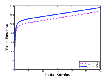
5.1.1 Total expected discounted value of all dividends versus initial surplus

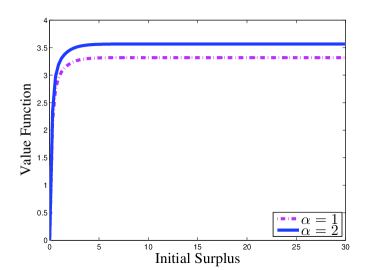
5.1.2 Differential marginal yield versus initial surplus

Figure 5.1: Proportional reinsurance with exponential claim size distribution with two regimes

   

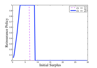
5.1.3 Optimal reinsurance policy to total expected discounted value of all dividends versus initial surplus

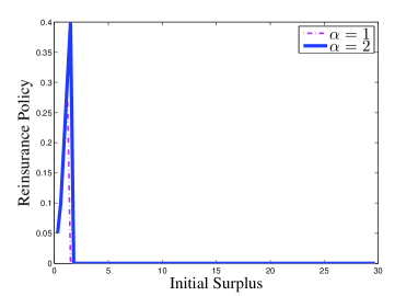
5.1.4 Optimal reinsurance policy to differential marginal yield versus initial surplus

Example 5.2.

In this example, the claim size distribution is assumed to be uniform in $[0,1]$. Then $E[Y]=\frac{1}{2}$ and $E[Y^{2}]=\frac{1}{3}$. Then the dynamic systems follows

$$\begin{array}[]{rl}\begin{cases}dX(t)=\frac{1}{2}\beta(\alpha(t))u(t)dt+\sqrt{\frac{1}{3}\beta(\alpha(t))}u(t)dw(t)-dZ(t),\\ X(0^{-})=x.\end{cases}\end{array}$$

Using the same data and payoff function in Example 5.1, we then obtained Figure 25.2.4.

   

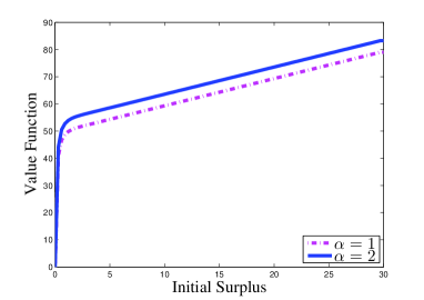
5.2.1 Total expected discounted value of all dividends versus initial surplus

5.2.2 Differential marginal yield versus initial surplus

Figure 5.2: Proportional reinsurance with uniform claim size distribution with two regimes

   

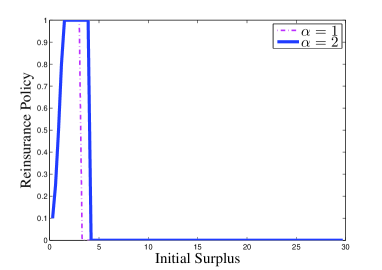
5.2.3 Optimal reinsurance policy to total expected discounted value of all dividends versus initial surplus

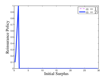
5.2.4 Optimal reinsurance policy to differential marginal yield versus initial surplus

5.2 Excess-of-Loss Reinsurance

Example 5.3.

Comparing to Example 5.1 and Example 5.2, the retention level $u(t)$ describes the maximal amount paid by the cedent for each claim. Assume the claim size distribution to be exponential with parameter 1 and $Q$, $\beta(1),\beta(2)$ and payoff functions to be the same as those in Example 5.1. Intuitively, the retention level cannot be arbitrarily large, then we restrict the risk control set $U$ to be $[0,1]$. That is, the retention level should not exceed the mean value of the exponential distributed claim size. Following (1.3)

$$\begin{array}[]{ll}&\!\!\!\displaystyle E[Y^{u}]=\int_{0}^{u}e^{-x}dx=1-e^{-u},\\ &\!\!\!\displaystyle E[(Y^{u})^{2}]=\int_{0}^{u}2xe^{-x}dx=2[1-e^{-u}(1+u)].\end{array}$$

Then the dynamic systems satisfy

$$\left\{\begin{array}[]{ll}&\!\!\!\displaystyle dX(t)=\beta(\alpha(t))[1-e^{-u(t)}]dt+\sqrt{2\beta(\alpha(t))[1-e^{-u(t)}(1+u(t))]}dw(t)-dZ(t),\\ &\!\!\!\displaystyle X(0^{-})=x;\end{array}\right.$$

see Figure 35.3.2 for this case.

   

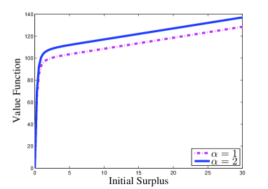
5.3.1 Total expected discounted value of all dividends versus initial surplus

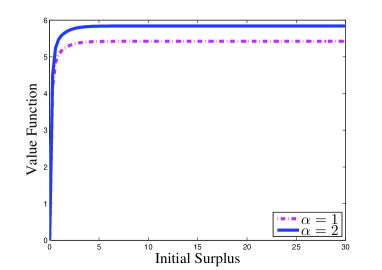
5.3.2 Differential marginal yield versus initial surplus

Figure 5.3: Excess-of-loss reinsurance with exponential claim size distribution with two regimes

   

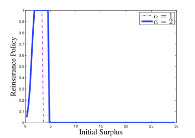
5.3.3 Optimal reinsurance policy to total expected discounted value of all dividends versus initial surplus

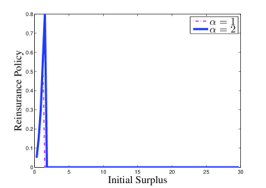
5.3.4 Optimal reinsurance policy to differential marginal yield versus initial surplus

Example 5.4.

Assume the claim size distribution to be uniform in $[0,1]$. Similarly, we obtain

$$\begin{array}[]{ll}&\!\!\!\displaystyle E[Y^{u}]=\int_{0}^{u}(1-x)dx=u-\frac{u^{2}}{2},\\ &\!\!\!\displaystyle E[(Y^{u})^{2}]=\int_{0}^{u}2x(1-x)dx=u^{2}\Big{[}1-\frac{2u}{3}\Big{]}.\end{array}$$

Hence, the dynamic systems satisfy

$$\left\{\begin{array}[]{ll}&\!\!\!\displaystyle dX(t)=\Big{[}\beta(\alpha(t))(u(t)-\frac{u(t)^{2}}{2})\Big{]}dt+\sqrt{\beta(\alpha(t))u(t)^{2}\Big{[}1-\frac{2u(t)}{3}\Big{]}}dw(t)-dZ(t),\\ &\!\!\!\displaystyle X(0^{-})=x.\end{array}\right.$$

Let the risk control set $U=[0,1]$. We obtain Figure 5.4 in this case.

       

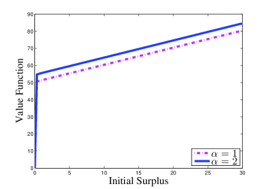
5.4.1 Total expected discounted value of all dividends versus initial surplus

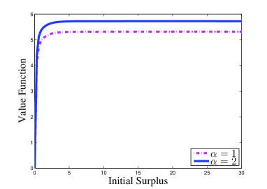
5.4.2 Differential marginal yield versus initial surplus

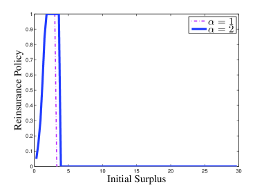
5.4.3 Optimal reinsurance policy to total expected discounted value of all dividends versus initial surplus

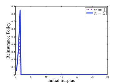
5.4.4 Optimal reinsurance policy to differential marginal yield versus initial surplus

Figure 5.4: Excess-of-loss reinsurance with uniform claim size distribution with two regimes

All of the figures contain two lines since we consider the two-regime case. Figures 15.1.1, 25.2.1, 35.3.1 and 45.4.1 show that the value function is concave and the dividend payout strategy is a barrier strategy. It is clear that if the surplus is higher than some barrier level, the extra surplus will be paid as the dividend, with the same time the value functions increase with unity slope.

Regarding the reinsurance policy, it is demonstrated in Figures 15.1.3, 25.2.3, 35.3.3, and 45.4.3 that both the proportional reinsurance and excess-of-loss reinsurance increase at first, maintain the highest rate in an interval, and decrease sharply to zero at a threshold to maximize the total expected discounted value of all dividends. From Figures 15.1.4, 25.2.4, 35.3.4, 45.4.4, in the case of maximizing the differential marginal yield, it is shown that both the proportional reinsurance and excess-of-loss reinsurance have similar trend comparing to the case of maximizing the total expected discounted value of all dividends, except that there are not the interval to hold the highest reinsurance rate. Furthermore, it is shown that in both regimes, there exists a free boundary (barrier) that separates two regions where the regular control or singular control is dominant. Also, the barrier levels are different in different regimes due to the Markov switching.

In addition, we compare the values for proportional reinsurance and excess-of-loss reinsurance with exponential claim size distribution in Table 5.1. At the level of initial surplus $x=30$, we compare the corresponding values in two regimes. Similarly we have the comparison in Table 5.2 for the uniform claim size distribution.

Reinsurance type	$\alpha=1$	$\alpha=2$
proportional reinsurance	127.661229	136.139963
excess-of-loss reinsurance	128.207117	136.686110

Table 5.1: $V(30,\alpha)$ with exponential claim size distribution for proportional reinsurance and excess-of-loss reinsurance

Reinsurance type	$\alpha=1$	$\alpha=2$
proportional reinsurance	79.010314	83.256482
excess-of-loss reinsurance	80.097716	84.302264

Table 5.2: $V(30,\alpha)$ with uniform claim size distribution for proportional reinsurance and excess-of-loss reinsurance

From Tables 5.1 and 5.2, we see that $V(30,\alpha)$ of excess-of-loss reinsurance are bigger than that of proportional reinsurance in both of the two regimes. That is, we can conclude that the excess-of-loss reinsurance is more profitable than proportional reinsurance under the same condition. This is consistent with the one regime case in Asmusen et al., (2000). Finally, the numerical method can treat complicate cost functions such as the marginal yield, which is another advantage of the numerical solutions.

6 Further Remark

In this work, we have developed a numerical approximation scheme to maximize the payoff function of the total discounted dividend paid out until the lifetime of ruin. A generalized formulation of reinsurance and dividend pay-out strategy is presented. Although one could derive the associated system of QVIs by using the usual dynamic programming approach together with the use of properties of regime-switchings, solving for the mixed regular-singular control problem analytically is very difficult. As an alternative, we presented a Markov chain approximation method using mainly probabilistic methods. For the singular control part, a technique of time rescaling is used. In the actual computation, the optimal value function can be obtained by using the value or policy iteration methods. Examples of proportional and excess-of-loss reinsurance are presented with more complicated payoff functions.

Appendix A Appendix: Proof of Proposition 4.3

The proof is similar in spirit to Yin et al., (2009) however regime-switching is included. The technique are originated from the work of Kushner and Dupuis, (2001). For simplicity, We divide the proofs into several steps. First, for any $\varsigma>0$, by Theorem 4.2, there are $\varepsilon>0$, a finite set $U^{\varsigma}\subset U$, and a probability space on which are defined a solution in the stochastic differential equation in (2.1). Thus, we have $(x^{\varsigma}(\cdot),\alpha^{\varsigma}(\cdot),u^{\varsigma}(\cdot),w^{\varsigma}(\cdot))$, where $U^{\varsigma}(\cdot)$ is $U^{\varsigma}$-valued and constant on $[n\varepsilon,n\varepsilon+\varepsilon)$. Moreover, $(x^{\varsigma}(\cdot),\alpha^{\varsigma}(\cdot),m^{\varsigma}(\cdot),w^{\varsigma}(\cdot))$ converges weakly to $(X(\cdot),\alpha(\cdot),m(\cdot),w(\cdot))$, the solution of the differential equation in (2.1). This further implies that $\limsup_{\varsigma}|J^{m^{\varsigma}}_{x,\iota}(\cdot)-J^{m}_{x,\iota}(\cdot)|\leq\varepsilon_{\widetilde{\varsigma}}$ with $\varepsilon_{\widetilde{\varsigma}}$ satisfying $\varepsilon_{\widetilde{\varsigma}}\to 0$ as $\widetilde{\varsigma}\to 0$.

Next, consider a $u^{\varsigma}(\cdot)$ for $\varsigma$ sufficiently small. Let $0<\theta<\varepsilon$. For $\phi\in U^{\varsigma}$, define the function $F_{n,\theta}$ as the regular conditional probability

$$\begin{array}[]{rl}&\!\!\!\displaystyle F_{n,\theta}(\phi,u^{\varsigma}(i\varepsilon),i<n,w^{\varsigma}(p\theta),p\theta\leq n\varepsilon)=P(u^{\varsigma}(n\varepsilon)=\phi|u^{\varsigma}(i\varepsilon),i<n,w^{\varsigma}(p\theta),p\theta\leq n\varepsilon).\end{array}$$

The uniqueness of the solution of the wealth equation or the associated martingale problem implies that the law of $(x^{\varsigma},\alpha^{\varsigma}(\cdot),m^{\varsigma}(\cdot),w^{\varsigma}(\cdot))$ is determined by the law of $(\alpha^{\varsigma}(\cdot),m^{\varsigma}(\cdot),w^{\varsigma}(\cdot))$ since the $\sigma$-algebra determined by $\{u^{\varsigma}(i\varepsilon),i<n,w^{\varsigma}(p\theta),\alpha^{\varsigma}(p\theta),p\theta\leq n\varepsilon\}$ increases to the $\sigma$-algebra determined by $\{u^{\varsigma}(i\varepsilon),i<n,w^{\varsigma}(\tau),\alpha^{\varsigma}(\tau),\tau\leq n\varepsilon\}$ as $\theta\to 0$, we can show that for each $n$, $\phi$, and $\varepsilon$, $F_{n,\theta}(\phi,u^{\varsigma}(i\varepsilon),i<n,w^{\varsigma}(p\theta),\alpha^{\varsigma}(p\theta),p\theta\leq n\varepsilon)\to P(u^{\varsigma}(n\varepsilon)=\phi|u^{\varsigma}(i\varepsilon),i<n,w^{\varsigma}(\tau),\alpha^{\varsigma}(\tau),\tau\leq n\varepsilon)$ with probability one as $\theta\to 0$.

For $w^{\varsigma,\theta}(\cdot)$, define the control $u^{\varsigma,\theta}(\cdot)$ by the conditional probability given in $F_{n,\theta}$ with $\varsigma$ replaced by $\varsigma,\theta$. Owing to the construction of the control law, as $\theta\to 0$, $(\alpha^{\varsigma,\theta}(\cdot),m^{\varsigma,\theta}(\cdot),w^{\varsigma,\theta}(\cdot))$ converges weakly to $(\alpha^{\varsigma}(\cdot),m^{\varsigma}(\cdot),w^{\varsigma}(\cdot))$. We can further show $(x^{\varsigma,\theta}(\cdot),\alpha^{\varsigma,\theta}(\cdot),m^{\varsigma,\theta}(\cdot),w^{\varsigma,\theta}(\cdot))$ converges weakly to $(x^{\varsigma}(\cdot),\alpha^{\varsigma}(\cdot),m^{\varsigma}(\cdot),w^{\varsigma}(\cdot))$ as $\theta\to 0$, and moreover $x^{\varsigma,\theta}(\cdot)$ converges weakly to $x^{\varsigma}(\cdot)$. Thus $|J^{m^{\varsigma,\theta}}_{x,\iota}(\cdot)-J^{m^{\varsigma}}_{x,\iota}(\cdot)|\leq g_{1}(\theta)$, where $g_{1}(\theta)\to 0$ as $\theta\to 0$.

For $\Delta>0$, consider the mollifier $F_{n,\theta,\Delta}(\cdot)$ given by

$$\begin{array}[]{rl}&\!\!\!\displaystyle F_{n,\theta,\Delta}(\phi;u(i\varepsilon),i<n,w(p\theta),p\theta\leq n\varepsilon)\\ &\!\!\!\displaystyle=N(\Delta)\int\cdots\int F_{n,\theta}(\phi;u(i\varepsilon),i<n,w(p\theta)+z_{p},p\theta\leq n\varepsilon)\times\prod_{p}\exp(-|z_{p}|^{2}/(2\Delta))dz_{p},\end{array}$$

where $N(\Delta)$ is a normalizing constant so the integral of the mollifier is unity. Note that $F_{n,\theta,\Delta}$ are nonnegative, and they are continuous in the $w$-variable. As $\Delta\to 0$, $F_{n,\theta,\Delta}$ converges to $F_{n,\theta}$ with probability one. Let $u^{\varsigma,\theta,\Delta}(\cdot)$ be the piecewise constant admissible control that is determined by the conditional probability distribution $F_{n,\theta,\Delta}(\cdot)$. There is a probability space on which we can define $w^{\varsigma,\theta,\Delta}(\cdot)$ and the control law $u^{\varsigma,\theta,\Delta}(\cdot)$ by the conditional probability

$$\begin{array}[]{rl}&\!\!\!\displaystyle P(u^{\varsigma,\theta,\Delta}(n\varepsilon)=\phi|u^{\varsigma,\theta,\Delta}(i\varepsilon),i<n,w^{\varsigma,\theta,\Delta}(\tau),\tau\leq n\varepsilon)\\ &\displaystyle\ =F_{n,\theta,\Delta}(\phi;u^{\varsigma\theta,\Delta}(i\varepsilon),i<n,w^{\varsigma,\theta,\Delta}(p\theta),p\theta\leq n\varepsilon).\end{array}$$

Then $(x^{\varsigma,\theta,\Delta}(\cdot),\alpha^{\varsigma,\theta,\Delta}(\cdot),m^{\varsigma,\theta,\Delta}(\cdot),w^{\varsigma,\theta,\Delta}(\cdot))$ converges weakly to $(x^{\varsigma,\theta}(\cdot),\alpha^{\varsigma,\theta},m^{\varsigma,\theta}(\cdot),w^{\varsigma,\theta}(\cdot))$ as $\Delta\to 0$. This yields that $|J^{m^{\varsigma,\theta,\Delta}}_{x,\iota}(\cdot)-J^{m^{\varsigma,\theta}}_{x,\iota}(\cdot)|\leq g_{2}(\Delta)$, where $g_{2}(\Delta)\to 0$ as $\Delta\to 0$.

Finally, choose $\widetilde{\varsigma}$ sufficiently small. Then for each $\varsigma>0$, there are $\varepsilon>0$, $\theta>0$, $w^{\varsigma}(\cdot)$, and an admissible control that is piecewise constant on $[n\varepsilon,n\varepsilon+\varepsilon)$ taking values in a finite set $U^{\varsigma}\subset U$ determined by the conditional probability law

$$\begin{array}[]{rl}&\!\!\!\displaystyle P(u^{\varsigma}(n\varepsilon)=\phi|u^{\varsigma}(i\varepsilon),i<n,w^{\varsigma}(\tau),\alpha^{\varsigma}(\tau),\tau\leq n\varepsilon)\\ &\displaystyle\ \ =F_{n}(\phi;u^{\varsigma}(i\varepsilon),i<n,w^{\varsigma}(p\theta),\alpha^{\varsigma}(p\theta),p\theta\leq n\varepsilon),\end{array}$$

where $F_{n}(\cdot)$ are continuous w.p.1 in the $w$-variables for each of other variables. Moreover, (4.16) holds. $\Box$

References

- (1)
- (2)
- Alvarez, (2000) Alvarez, L.H.R. (2000). Singular stochastic control in the presence of a state-dependent yield structure, Stochastic Process. Appl., 86: 323–343.
- Asmussen, (1989) Asmussen, A. (1989). Risk theory in a Markovian environment, Scand. Actur. J., (2):69–100.
- Asmusen et al., (2000) Asmussen, S., Høgaard, B., and Taksar, M. (2000). Optimal risk control and dividend distribution policies. Example of excess-of loss reinsurance for an insurance corporation. Finance and Stochastics, 4: 299–324.
- Asmussen and Taksar, (1997) Asmussen, S. and Taksar, M. (1997). Controlled diffusion models for optimal dividend pay-Out. Insurance: Math. and Economics, 20: 1–15.
- Bayraktar et al., (2011) Bayraktar, E., Song, Q.S., and Yang, J. (2011), On the continuity of stochastic exit time control problems, Stoch. Anal. Appl., 29(1):48–60.
- Browne, (1995) Browne, S. (1995). Optimal investment policies for a firm with a random risk process: Exponential utility and minimizing the probability of ruin. Mathematics of Operations Research 20(4): 937–958.
- Browne, (1997) Browne, S. (1997). Survival and growth with liability optimal portfolio strategies in continuous time. Mathematics of Operations Research 22(2): 468–493.
- Budhiraja and Ross, (2007) Budhiraja, A. and Ross, K. (2007). Convergent numerical scheme for singular stochastic control with state constraints in a portfolio selection problem. SIAM J. Control Optim., 45(6):2169– 2206.
- Choulli et al., (2001) Choulli, T., Taksar, M. and Zhou, X. Y. (2001). Excess-of-loss reinsurance for a company with debt liability and constraints on risk reduction. Quant. Finance 1:573–96.
- De Finetti, (1957) De Finetti, B. (1957). Su unimpostazione alternativa della teoria collettiva del rischio. Transactions of the XVth International Congress of Actuaries 2: 433–443.
- Fleming and Soner, (2006) Fleming, W. and Soner, H. (2006). Controlled Markov Processes and Viscosity Solutions, volume 25 of Stochastic Modelling and Applied Probability. Springer-Verlag, New York, NY, second edition.
- Gerber and Shiu, (2004) Gerber, H. and Shiu, E. (2004). Optimal dividends: analysis with Brownian motion. North American Actuarial Journal, 8: 1–20.
- Gerber and Shiu, (2005) Gerber, H. and Shiu, E (2005). On optimal dividends: From reflection to refraction. Journal of Computational and Applied Mathematics, 186: 4–22.
- Gerber and Shiu, (2006) Gerber, H. and Shiu, E. (2006). On optimal dividend strategies in the compound Poisson model. North American Actuarial Journal, 10: 76–93.
- Hamilton, (1989) Hamilton, J. (1989). A new approach to the economic analysis of non-stationary time series. Econometrica, (57): 357–384.
- Jin et al., (2011) Jin, Z., Yin, G. and Yang, H.L. (2011). Numerical methods for dividend optimization using regime-switching jump-diffusion models. Mathematical Control and Related Fields, 1: 21-40.
- Kushner, (1990) Kushner, H. (1990). Weak Convergence Methods and Singularly Perturbed Stochastic Control and Filtering Problems, Birkhäuser, Boston, MA.
- Kushner and Dupuis, (2001) Kushner, H. and Dupuis, P. (2001). Numerical Methods for Stochstic Control Problems in Continuous Time, volume 24 of Stochastic Modelling and Applied Probability. Springer, New York, second edition.
- Kushner and Martins, (1991) Kushner, H. J. and Martins, L. F. (1991). Numerical methods for stochastic singular control problems. SIAM J. Control Optim., 29:1443–475.
- Lundberg, (1903) Lundberg, F. (1903). Approximerad Framställning av Sannolikehetsfunktionen, Aterförsäkering av Kollektivrisker, Almqvist & Wiksell, Uppsala. Akad. Afhandling. Almqvist o. Wiksell, Uppsala.
- Ma and Yong, (1999) Ma, J. and Yong, J. (1999). Dynamic programming for multidimensional stochastic control problems. Acta Math. Sin., 15(4):485–506.
- Pham, (2009) Pham, H. (2009). Continuous-time stochastic control and optimization with financial applications, volume 61 of Stochastic Modelling and Applied Probability. Springer-Verlag, Berlin.
- Sotomayor and Cadenillas, (2011) Sotomayor, L. and Cadenillas, A. (2011) Classical, singular, and impulse stochastic control for the optimal dividend policy when there is regime switching. Insurance: Mathematics and Economics, 48(3), 344–54
- Wei et al., (2010) Wei, J., Yang, H. and Wang, R. (2010). Classical and impulse control for the optimization of dividend and proportional reinsurance policies with regime switching. Journal of Optimization Theory and Applications, 147(2).
- Yang and Yin, (2004) Yang, H and Yin, G. (2004), Ruin probability for a model under Markovian switching regime, In T.L. Lai, H. Yang, and S.P. Yung, editors, Probability, Finance and Insurance, pages 206–217. World Scientific, River Edge, NJ.
- Yin et al., (2009) Yin, G., Jin, H., and Jin, Z. (2009). Numerical methods for portfolio selection with bounded constraints. J. Computational Appl. Math., 233: 564–581.
- Yin et al., (2003) Yin, G., Zhang, Q., Badowski, G. (2003). Discrete-time singularly perturbed Markov chains: Aggregation, occupation measures, and switching diffusion limit. Advances in Applied Probability, 35:449–476.
- Yin and Zhu, (2010) Yin, G. and Zhu, C. (2010). Hybrid Switching Diffusions: Properties and Applications. Springer, New York, 2010.
- (31)