Bondi-Sachs energy-momentum for the constant mean extrinsic curvature initial value problem

Abstract

The constraints on the asymptotic behavior of the conformal factor and conformal extrinsic curvature imposed by the initial value equations of general relativity on constant mean extrinsic curvature (CMC) hypersurfaces are analyzed in detail. We derive explicit formulas for the Bondi-Sachs energy and momentum in terms of coefficients of asymptotic expansions on CMC hypersurfaces near future null infinity. Precise numerical results for the Bondi-Sachs energy, momentum, and angular momentum are used to interpret physically Bowen-York initial data on conformally flat CMC hypersurfaces similar to that calculated earlier by Buchman et al. [1].

I Introduction

Recently, there has been increased interest in formulations for numerical relativity based on conformal compactification [2] in which the calculational grid extends to future null infinity ($\mathscr{I}^{+}$), where the gravitational radiation amplitude can be read off unambiguously, with at most numerical errors, and where no dynamical boundary conditions are necessary. In principle this can be done with Cauchy characteristic matching methods, but these have not been implemented successfully with non-trivial dynamics. Cauchy characteristic extraction methods can extrapolate from the outer boundary of a conventional Cauchy code to determine waveforms at $\mathscr{I}^{+}$, but do not eliminate errors in the Cauchy development deriving from inexact boundary conditions at a finite radius. The characteristic methods are reviewed by J. Winicour [3]. Our focus here is the initial value problem on hyperboloidal spacelike hypersurfaces, and specifically the case of constant mean extrinsic curvature (CMC) hypersurfaces [4, 5, 6, 7, 8]. The vanishing of the conformal factor $\Omega$ at $\mathscr{I}^{+}$ accounts for the singular behavior of the physical spacetime metric at $\mathscr{I}^{+}$ in compactified coordinates. The conformal geometry, in which $\mathscr{I}^{+}$ is an ingoing null hypersurface, is regular in a neighborhood of $\mathscr{I}^{+}$, and a CMC hypersurface of the physical spacetime is spacelike in the conformal spacetime out to and including its intersection with $\mathscr{I}^{+}$, a 2-surface with spherical topology which we denote by $\dot{\mathscr{I}^{+}}$. Regularity conditions relating the 2D extrinsic curvature of $\dot{\mathscr{I}^{+}}$ as embedded in the CMC hypersurface to the conformal extrinsic curvature need to be satisfied at $\dot{\mathscr{I}^{+}}$, but when imposed in the initial data are automatically preserved by the evolution equations [5, 8]. The constraint equations, given suitable gauge conditions, determine the leading behavior of the conformal factor and the conformal extrinsic curvature of the hypersurface in the neighborhood of $\mathscr{I}^{+}$ in terms of asymptotic gravitational wave amplitudes [9]. If the physical mean extrinsic curvature is not too large, the dynamics of the sources (black holes, neutron stars) takes place where the CMC hypersurfaces are not that different from the hypersurfaces of conventional 3+1 methods.

Conformally flat initial data on CMC hypersurfaces were considered in Ref. [1]. The conformal momentum constraint equations have the same form as they do on maximal hypersurfaces, and with conformal flatness admit a class of analytic solutions which are slight generalizations of the well-known Bowen-York solutions [10] often used for single or multiple black hole initial data on maximal hypersurfaces. The Hamiltonian constraint provides an elliptic equation for the conformal factor which is degenerate at $\mathscr{I}^{+}$. Despite this degeneracy, Ref. [1] obtained numerical solutions without much difficulty using the standard spectral elliptic solver of the Caltech-Cornell-CITA SpEC code [11, 12]. The degeneracy constrains the leading terms in the expansion of $\Omega$ about $\dot{\mathscr{I}^{+}}$.

An essential part of the physical interpretation of these solutions is knowing precisely the total energy, linear momentum, and angular momentum of the system as coded in the asymptotic behavior of the spacetime metric at $\mathscr{I}^{+}$. The standard Arnowitt-Deser-Misner (ADM) formulas [13] for these quantities only apply on asymptotically flat slices at spatial infinity. The Bondi-Sachs energy and momentum at $\mathscr{I}^{+}$ [14, 15] are the relevant quantities for CMC hypersurfaces. Ref. [1] did not fully address this issue, making only some rather crude estimates of the total energy, momentum, and angular momentum with limited validity and for the most part with uncertain errors.

While there is an extensive literature dealing with the problem of extracting these global physical quantities near or at at future null infinity (see, e.g., the review [16]), part of which deals specifically with CMC hypersurfaces [17], we see practical difficulties in implementing many of these procedures. Some of them require the choice of a reference spatial metric and extrinsic curvature. Determining the reference quantities with the precision necessary to obtain unambiguous results requires considerable effort, in general. Formulas based on the asymptotic behavior of the Weyl tensor (e.g., [15, 18, 19]) can be useful computationally, but an analysis based on geometrically defined spatial coordinates gives more insight into the asymptotic geometry of CMC hypersurfaces and its relationship to the Bondi expansion on null hypersurfaces.

We first consider the problem of calculating the Bondi energy and momentum in general asymptotically flat spacetimes foliated by CMC hypersurfaces. Following Appendix A of Ref. [8], we analyze the asymptotic geometry using Gaussian normal spatial coordinates tied to the $\dot{\mathscr{I}^{+}}$ 2-surface. This gauge choice allows a relatively simple characterization of the asymptotic behavior of the spacetime metric and extrinsic curvature on a CMC hypersurface based on asymptotic solutions of the constraint equations. Constructing the asymptotic coordinate transformation from the CMC-based coordinates to Bondi-Sachs null coordinates gives us the Bondi-Sachs mass aspect in terms of geometric objects defined on a single CMC hypersurface. The monopole and dipole moments of the Bondi-Sachs mass aspect are the Bondi-Sachs energy and linear momentum, respectively. In the simple case of conformally flat initial data, the mass aspect is just a sum of contributions from the asymptotic expansions of the conformal factor and conformal extrinsic curvature.

The Bowen-York solutions for the conformal extrinsic curvature contain parameters such as boost and spin vectors, which on maximal hypersurfaces are simply related to the ADM momentum and angular momentum. On CMC hypersurfaces, the relationship of the Bowen-York parameters to physical momenta and energies is more complicated, but we are able to obtain analytic expressions for the direct contributions of the conformal extrinsic curvature to the Bondi-Sachs energy and momentum in terms of the Bowen-York parameters. Unlike on maximal hypersurfaces, on conformally flat CMC hypersurfaces the coordinate displacement of the black hole from the center of the coordinate sphere representing $\mathscr{I}^{+}$ enters in a non-trivial way. The conformal factor contributions to the Bondi-Sachs energy and momentum are extracted from the numerical solution of the Hamiltonian constraint equation. We also derive an analytic expression for the total angular momentum of the system which only depends on the Bowen-York parameters, without any contribution from the conformal factor. We discuss the physical interpretation of some representative examples of Bowen-York initial data on CMC hypersurfaces similar to those of Ref. [1], and show how to construct initial data approximating a circular-orbit binary black hole system.

The Wald sign convention for the extrinsic curvature is adopted, so that the mean extrinsic curvature $K$ is positive for hypersurfaces with diverging future-directed normals, the hypersurfaces extending to future null infinity rather than to spatial infinity ($K=0$) or to past null infinity ($K<0$). Our notation is an amalgam of that of Refs. [1, 17] and very similar to that in Appendix A of Ref. [8], but be alert to occasional deviations. We assume vacuum in a neighborhood of future null infinity. The discussion of the asymptotic geometry on general CMC hypersurfaces is in Sec. II. In Sec. III, we use the lapse and shift which preserve the CMC hypersurface condition and the Gaussian normal spatial coordinate condition to facilitate the asymptotic transformation to Bondi-Sachs coordinates. The final expression for the mass aspect depends only on the geometric properties of a single CMC hypersurface. Numerical results for the generalized Bowen-York initial data on conformally flat CMC hypersurfaces are presented in Sec. IV. The implications of our results for astrophysically interesting initial data are summarized in Sec. V. In Appendix A, we derive the analytic expressions for the conformal extrinsic curvature contribution to Bondi-Sachs four-momentum and in Appendix B the analytic expression for the total angular momentum.

II Asymptotic behavior on CMC hypersurfaces

The fact that the Hamiltonian constraint equation for the conformal factor and the momentum constraint equation for the extrinsic curvature are degenerate at $\mathscr{I}^{+}$ means that the first few terms in a power series expansion of these quantities away from $\dot{\mathscr{I}^{+}}$ are uniquely determined from the expansion of the conformal spatial metric, in spite of the elliptic character of the equations and therefore the generally nonlocal character of the solutions. In our derivation of formulas for the Bondi-Sachs energy-momentum 4-vector, we will not assume the conformal spatial metric is flat, though all of our numerical examples are for the conformally flat case. The expansion parameter defined in Ref. [1] is only meaningful for a flat conformal spatial metric, so the analysis here follows the derivation of asymptotic behavior presented in Appendix A of Ref. [8], which in turn rather closely follows that of Ref. [9]. It is based on a particular choice of spatial coordinates, Gaussian normal coordinates, in which the “radial” coordinate $z$ is the conformal proper distance inward from $\dot{\mathscr{I}^{+}}$ along normal spatial geodesics in the CMC hypersurface considered as a slice of the conformal spacetime. As in Ref. [8], we assume that the intrinsic geometry of $\dot{\mathscr{I}^{+}}$ is that of a 2-sphere of fixed area in the conformal geometry, which can be enforced in any asymptotically flat spacetime by suitable boundary conditions on the initial conformal gauge and its subsequent evolution, at least if the gauge evolution variables are determined by elliptic equations, as in Refs. [5, 8]. Angular coordinates $x^{A}$ are propagated along the normal geodesics starting from standard polar angles on the $\dot{\mathscr{I}^{+}}$ two-sphere. While the actual computational coordinates will be different, in general, the coefficients in the expansions are expressed in terms of quantities defined covariantly and therefore can be computed in any coordinate system. An equality which holds only at $\mathscr{I}^{+}$ is indicated by a dot above the equal sign.

We just give the key definitions and results here, and refer the reader to Ref. [8] for details of the derivations. The conformal spacetime metric $\tilde{g}_{\mu\nu}$ is related to the physical spacetime metric $g_{\mu\nu}$ by

$$\tilde{g}_{\mu\nu}=\Omega^{2}g_{\mu\nu},$$

and a tilde will be used generally to distinguish quantities associated with the conformal, rather than the physical, geometry. The conformal factor is required to vanish on $\mathscr{I}^{+}$, where it cancels the infinities in the physical metric due to the compactified spatial coordinates and the CMC hypersurfaces becoming asymptotically null, and is strictly positive in the interior. The general form of the conformal spatial metric in Gaussian normal coordinates is

$$\tilde{g}_{ij}dx^{i}dx^{j}=dz^{2}+\tilde{h}_{AB}dx^{A}dx^{B},$$ (1)

with $z=0$ at $\dot{\mathscr{I}^{+}}$. A metric function $\xi$ is defined such that $\det\tilde{h}_{AB}=\xi^{-4}\sin^{2}\theta$. At $\dot{\mathscr{I}^{+}}$, $\tilde{h}_{AB}\doteq\xi_{0}^{-2}\breve{h}_{AB}$, with $\breve{h}_{AB}$ the standard metric of the unit two-sphere in polar coordinates. We require that $\xi_{0}$ be independent of angle. Then the 2D scalar curvature of $\dot{\mathscr{I}^{+}}$ is $2\xi_{0}^{2}$. The only way to preserve this property of $\dot{\mathscr{I}^{+}}$ is to demand that $\partial_{t}\xi_{0}=0$ during the evolution as a condition on the evolution of the conformal gauge. We can keep the CMC time coordinate $t$ equal to a Minkowski retarded time coordinate $u$ at $\mathscr{I}^{+}$ by imposing the boundary condition $\tilde{\alpha}\doteq K/(3\xi_{0})\equiv\tilde{\alpha}_{0}$ on the elliptic equation for the conformal lapse which follows from $\partial_{t}K=0$.

A general form for the expansion of $\tilde{h}_{AB}$ in powers of $z$ away from $\dot{\mathscr{I}^{+}}$ is then

$$\tilde{h}_{AB}=\xi^{-2}\left[\breve{h}_{AB}-2\breve{\chi}_{AB}z+\left(\breve{\chi}^{CD}\breve{\chi}_{CD}\breve{h}_{AB}-\breve{\psi}_{AB}\right)z^{2}+O(z^{3})\right].$$ (2)

Here $\breve{\chi}_{AB}$ and $\breve{\psi}_{AB}$ are traceless, symmetric tensors on the unit sphere with indices lowered and raised by $\breve{h}_{AB}$ and its inverse. Note the identity that $\breve{\chi}_{A}^{\;C}\,\breve{\chi}_{CB}\equiv\frac{1}{2}\breve{\chi}^{CD}\breve{\chi}_{CD}\breve{h}_{AB}$. As argued in Ref. [8], we believe it is consistent and physically appropriate in the context of gravitational radiation generated by the internal dynamics of isolated systems not to allow any polyhomogeneous terms, that is, terms containing powers of $\log{z}$ as well as powers of $z$, to this order in the expansion. The expansion of $\tilde{h}_{AB}$ is closely related to the expansion of the angular part of the metric in Bondi-Sachs coordinates. Ref. [20] showed that the coefficient of the leading polyhomogeneous term of order $r^{-1}\log r$ or $r^{-2}\log r$ in the Bondi expansion is a constant of the motion, so if these terms are absent initially they never appear. If these polyhomogeous terms are not present in the Bondi expansion, the corresponding terms are not present in Eq. 2. The inverse of the angular part of the metric is

$$\tilde{h}^{AB}=\xi^{2}\left[\breve{h}^{AB}+2\breve{\chi}^{AB}z+\left(\breve{\chi}^{CD}\breve{\chi}_{CD}\breve{h}^{AB}+\breve{\psi}^{AB}\right)z^{2}+O(z^{3})\right].$$ (3)

The angular metric functions can be related to the extrinsic curvature $\tilde{\kappa}^{A}_{B}$ of the constant-$z$ two-surfaces as embedded in the 3D conformal geometry of the CMC hypersurface. The trace of the 2D extrinsic curvature is $\tilde{\kappa}=2\partial_{z}(\log{\xi})$, and the traceless part is

$$\hat{\tilde{\kappa}}^{A}_{B}=\breve{\chi}^{A}_{B}+\breve{\psi}^{A}_{B}z+O(z^{2}).$$

The expansion of $\xi$ as a power series in $z$ can be expressed in terms of the expansion of $\tilde{\kappa}$,

$$\tilde{\kappa}=\tilde{\kappa}_{0}+\tilde{\kappa}_{1}z+\tilde{\kappa}_{2}z^{2}+O(z^{3}),$$

with the result

$$\log{\xi}=\log{\xi_{0}}+\frac{1}{2}\tilde{\kappa}_{0}z+\frac{1}{4}\tilde{\kappa}_{1}z^{2}+\frac{1}{6}\tilde{\kappa}_{2}z^{3}+O(z^{4}).$$ (4)

Satisfying our condition on the intrinsic geometry of $\dot{\mathscr{I}^{+}}$ requires that $\xi_{0}$ be a constant, independent of both time and angle, but all of the coefficients in the expansion of $\tilde{\kappa}$ will in general depend on the time $t$ and the angular coordinates $x^{A}$. The 2D extrinsic curvature is a tensor which can be calculated in any coordinate system by solving the geodesic equations in the conformal spatial geometry.

A straightforward calculation gives the conformal 3D Ricci tensor components. The result is Eq. (A6) of Ref. [8],

$$\tilde{R}^{z}_{\,z} = \partial_{z}\tilde{\kappa}-\hat{\tilde{\kappa}}_{AB}\hat{\tilde{\kappa}}^{AB}-\frac{1}{2}\tilde{\kappa}^{2},$$

$$\tilde{R}^{z}_{\,A} = \frac{1}{2}\tilde{\kappa}_{|{A}}-\hat{\tilde{\kappa}}^{C}{}_{{A}|{C}},$$ (5)

$$\tilde{R}^{A}_{B} = \,\partial_{z}\hat{\tilde{\kappa}}^{A}_{B}-\tilde{\kappa}\,\hat{\tilde{\kappa}}^{A}_{B}+\frac{1}{2}\left({\,{}^{2}\tilde{R}+\partial_{z}\tilde{\kappa}-\tilde{\kappa}^{2}}\right)\delta^{A}_{B},$$

with

$$\,^{2}\tilde{R}^{A}_{B}=\frac{1}{2}\,\,^{2}\tilde{R}\,\delta^{A}_{B}=\xi_{0}^{2}\left[1+\left(\tilde{\kappa}_{0}+\frac{1}{2}\tilde{\kappa}_{0}{}^{\breve{\scriptscriptstyle{|}}C}{}_{\breve{\scriptscriptstyle{|}}C}-\breve{\chi}^{CD}{}_{\breve{\scriptscriptstyle{|}}CD}\right)z+O(z^{2})\right]\delta^{A}_{B}.$$ (6)

The $\scriptstyle{|}$ symbol denotes a covariant derivative with respect to the metric $\tilde{h}_{AB}$ of the constant-$z$ two-surface, while the $\breve{\scriptscriptstyle{|}}$ symbol denotes a covariant derivative on the unit sphere. The curvature scalar evaluated at $\dot{\mathscr{I}^{+}}$ is

$$\tilde{R}\doteq 2\xi_{0}^{2}+2\tilde{\kappa}_{1}-\frac{3}{2}\tilde{\kappa}_{0}^{2}-\breve{\chi}^{AB}\breve{\chi}_{AB}.$$ (7)

We define the 3D conformal extrinsic curvature $\tilde{K}_{ij}$ to have the same relationship to the time derivative of the conformal spatial metric, the conformal lapse, and the shift as the physical extrinsic curvature $K_{ij}$ has to the time derivative of the physical spatial metric, the physical lapse, and the shift. This corresponds to the convention in Ref. [8] and the usual convention in the literature, but differs from Ref. [1]. The conformal extrinsic curvature is decomposed into its trace $\tilde{K}$ and traceless part $\hat{\tilde{K}}_{ij}$. The sign of the extrinsic curvature is that of Wald, with $K>0$ on a CMC hypersurface extending to $\mathscr{I}^{+}$.

The initial value equations on a CMC hypersurface constrain $\hat{\tilde{K}}_{ij}$ through the momentum constraint. The well-known “zero-shear” condition necessary for $\mathscr{I}^{+}$ to exist as a regular null hypersurface in the conformal manifold, expressed in our coordinates, says that

$$\Sigma^{A}_{B}\equiv\hat{\tilde{K}}^{A}_{B}-\frac{1}{2}\delta^{A}_{B}\hat{\tilde{K}}^{C}_{C}\doteq\hat{\tilde{\kappa}}^{A}_{B}\doteq\breve{\chi}^{A}_{B},\qquad\hat{\tilde{K}}^{z}_{A}\doteq\hat{\tilde{K}}^{z}_{z}\doteq 0.$$ (8)

The Hamiltonian constraint equation is an elliptic equation for $\Omega$, degenerate at $\dot{\mathscr{I}^{+}}$, where $\Omega\doteq 0$. The degeneracy allows no freedom in the first few terms of the expansion of the solution in powers of $z$. The asymptotic solution from Ref. [8] is

$$\Omega=\frac{K}{3}z\left[1-\frac{1}{4}\tilde{\kappa}_{0}z+\frac{1}{6}\left(\xi_{0}^{2}+\frac{1}{4}\tilde{\kappa}_{0}^{2}-\tilde{\kappa}_{1}-\breve{\chi}^{AB}\breve{\chi}_{AB}\right)z^{2}+\left(c_{3}+\frac{1}{8}Q\log{\frac{Kz}{3}}\right)z^{3}+O(z^{4})\right],$$ (9)

where $c_{3}$ is a function of angle only known from the global (numerical) solution of the elliptic equation and

$$Q\equiv\xi_{0}^{2}\left[\breve{\chi}^{AB}{}_{\breve{\scriptscriptstyle{|}}AB}+\breve{\chi}^{A}_{B}\left(\breve{\psi}^{B}_{A}-\frac{1}{2}\tilde{\kappa}_{0}\breve{\chi}^{B}_{A}\right)\right].$$ (10)

The logarithmic term is present whenever outgoing radiation is present at $\mathscr{I}^{+}$. It is a consequence of the CMC hypersurface condition. The coefficient $Q$ also appears in the asymptotic expansion of the conformal extrinsic curvature derived from the momentum constraint equation:

$$\hat{\tilde{K}}^{z}_{z}=\breve{\chi}^{A}_{B}\breve{\chi}^{B}_{A}z+\left(d_{1}-Q\log{\frac{Kz}{3}}\right)z^{2}+O(z^{3}).$$ (11)

If, in addition to the zero-shear condition, we require that the Weyl tensor vanish at $\mathscr{I}^{+}$, the expansion of $\Sigma^{A}_{B}$ is

$$\Sigma^{A}_{B}=\breve{\chi}^{A}_{B}+\frac{1}{2}\tilde{\kappa}_{0}\breve{\chi}^{A}_{B}z+O(z^{2}),$$ (12)

and the expansion of $\hat{\tilde{K}}^{z}_{A}$ is

$$\hat{\tilde{K}}^{z}_{A}=\breve{\chi}^{B}_{A\breve{\scriptscriptstyle{|}}B}z+e_{1}z^{2}+O(z^{3}).$$ (13)

The coefficients $d_{1}$ and $e_{1}$ are functions of angle which are known only from a global solution of the momentum constraint equation. The vanishing of the Weyl tensor at $\mathscr{I}^{+}$, called the Penrose regularity condition in Ref.  [8], is a necessary condition for the absence of polyhomogeneous terms in the Bondi-Sachs asymptotic expansion based on special null coordinates (see Ref. [15]).

The time evolution of the conformal factor $\Omega$ is given by

$$\partial_{t}\Omega=\beta^{k}\partial_{k}\Omega-\frac{1}{3}\tilde{\alpha}\left(K-\Omega\tilde{K}\right),$$ (14)

from which we see that $\tilde{K}$ controls how the conformal gauge evolves. We want the conformal gauge to be consistent with $\dot{\mathscr{I}^{+}}$ being a two-sphere at the coordinate position $z=0$ at all times. Keeping $\mathscr{I}^{+}$ at $z=0$ requires the boundary condition $\beta^{z}\doteq\tilde{\alpha}\doteq\tilde{\alpha}_{0}$ on the shift, so $\partial_{t}\Omega=0$ at $z=0$. The only way to make sure that $\xi_{0}$ stays independent of angle is to require that $\partial_{t}\xi_{0}=0$. We also require $\beta^{A}\doteq 0$, in order that the angular coordinates be propagated along the null generators of $\mathscr{I}^{+}$. These conditions greatly simplify the identification of the Bondi-Sachs mass aspect from the asymptotic behavior, since they make our coordinates close to inertial Bondi coordinates, for which the Bondi-Sachs mass aspect can be read off directly from the asymptotic expansion of the Bondi-Sachs metric.

The evolution equation for $\xi$, obtained from the evolution equation for the determinant of the angular part of the conformal metric in terms of the conformal extrinsic curvature, is

$$\partial_{t}(\log{\xi})=\beta^{k}\partial_{k}(\log{\xi})-\frac{1}{2}\beta^{C}{}_{\breve{\scriptscriptstyle{|}}C}+\tilde{\alpha}\left(\frac{1}{2}\hat{\tilde{K}}^{z}_{z}-\frac{1}{3}\tilde{K}\right),$$ (15)

where $\beta^{C}{}_{\breve{\scriptscriptstyle{|}}C}$ is the divergence of the angular part of the shift considered as a vector field on the unit sphere. At $\dot{\mathscr{I}^{+}}$, this becomes

$$\partial_{t}(\log{\xi})\doteq\tilde{\alpha}_{0}\left(\frac{1}{2}\tilde{\kappa}-\frac{1}{3}\tilde{K}\right).$$ (16)

Therefore, we impose the boundary condition

$$\tilde{K}\doteq\frac{3}{2}\tilde{\kappa}_{0}.$$ (17)

We make no other restrictions on the conformal gauge, i.e., on the details of the equation for $\tilde{K}$. As long as the equation is elliptic, as in Refs. [8] and [5], the boundary condition is easily enforced. If the conformal gauge is evolved as part of a purely hyperbolic system, in which there are no boundary conditions at $\mathscr{I}^{+}$, things may not be so simple.

III The Bondi-Sachs energy and momentum

The Bondi-Sachs energy is the true physical energy defined at future null infinity in asymptotically flat spacetimes. Its original definition [14, 15] was based on a special class of retarded null coordinates $\left(u,r,\bar{\theta},\bar{\phi}\right)$ with a metric of the form, in close to the notation of Ref. [9],

$$ds^{2}=-Ve^{2\beta}du^{2}-2e^{2\beta}dudr+r^{2}\bar{h}_{AB}\left({d\bar{x}^{A}-U^{A}du}\right)\left({d\bar{x}^{B}-U^{B}du}\right),$$

where $\bar{h}_{AB}$ is a 2D metric asymptotically approaching the unit sphere metric $\breve{h}_{AB}$ and whose determinant equals the determinant of $\breve{h}_{AB}$ everywhere. We put bars on the angular coordinates to distinguish them from the angular coordinates in the CMC hypersurface. The expansion of $\bar{h}_{AB}$ in powers of $x\equiv r^{-1}$ away from $\mathscr{I}^{+}$ has the form

$$\bar{h}_{AB}=\breve{h}_{AB}+\bar{\chi}_{AB}x+\frac{1}{4}\bar{\chi}^{CD}\,\bar{\chi}_{CD}\,\breve{h}_{AB}x^{2}+O(x^{3}).$$ (18)

The absence of any traceless contribution to the $O(x^{2})$ term in Eq. (18) implies the vanishing of the Weyl tensor on $\mathscr{I}^{+}$, as Eq. (12) did on CMC hypersurfaces. The remaining metric functions are asymptotically

$$V=1-2\,M\left(u,\bar{\theta},\bar{\varphi}\right)\,x+O(x^{2}),$$ (19)

$$\beta=-\frac{1}{{32}}\,\bar{\chi}^{BC}\,\bar{\chi}_{BC}\,x^{2}+O(x^{3}),$$ (20)

$$U^{A}=-\frac{1}{2}\,\bar{\chi}^{AB}{}_{\breve{\scriptscriptstyle{|}}{B}}\,x^{2}+O(x^{3}).$$ (21)

Like $\breve{\chi}_{AB}$, $\bar{\chi}_{AB}\left(u,\bar{\theta},\bar{\varphi}\right)$ is a traceless symmetric tensor on the unit sphere. Its retarded time derivative along $\mathscr{I}^{+}$ is the Bondi news.

The Bondi-Sachs metric function $M\left(u,\bar{\theta},\bar{\varphi}\right)$ is what was originally identified as the Bondi mass aspect [14]. Its average over the unit sphere at a fixed retarded time $u$ is the Bondi-Sachs energy $E_{\rm BS}$ and the average over the unit sphere weighted by $N^{i}$, where

$$N^{i}\equiv(\sin{\theta}\cos{\varphi},\sin{\theta}\sin{\varphi},\cos{\theta}),$$ (22)

is the $i$th component of of the Bondi-Sachs momentum three-vector in the asymptotic Minkowski frame. However, there are other less coordinate-specific definitions of the mass aspect which give the same Bondi-Sachs energy and momentum when averaged. Some are based on the asymptotic behavior of Weyl tensor [15, 21, 22, 19] and some are based on charge integrals derived from a Hamiltonian formalism (see, e.g., [23, 17]). What we will call the Bondi-Sachs mass aspect is not the metric function $M$, but rather the quantity which is monotonically decreasing on each of the null generators of $\mathscr{I}^{+}$ [23],

$$M_{\rm A}\equiv M-\frac{1}{4}\bar{\chi}^{AB}{}_{\breve{\scriptscriptstyle{|}}AB}.$$ (23)

The monopole and dipole angular moments of $M_{\rm A}$ and $M$ are identical for arbitrary $\bar{\chi}^{\rm AB}$ [17].

The task of actually calculating $M_{\rm A}$ from data on a CMC hypersurface can be accomplished in various ways. The charge integrals of Ref. [17] require comparing the actual spatial metric and extrinsic curvature on the hypersurface with a background metric and extrinsic curvature. The results are sensitive to the choice of background quantities. The only fail-safe procedure mentioned in Ref. [17] is to find the coordinate transformation from the CMC coordinates to Bondi coordinates, where the appropriate background spacetime metric is known, and then perform the inverse of this coordinate transformation on the Bondi-Sachs background metric. However, once one has transformed to Bondi coordinates, it is much simpler just to read off the Bondi-Sachs metric function $M$ from the transformed metric. It is the latter procedure that we will follow. While the coordinate transformation involves the lapse and shift for the CMC coordinates, the final result only depends on the spatial metric and extrinsic curvature of a single CMC hypersurface.

The lapse and shift which preserve the CMC slicing condition and the Gaussian normal coordinates based on $\dot{\mathscr{I}^{+}}$ were derived in Appendix A of Ref. [8]. The singular terms in the elliptic equation for the conformal lapse allow no freedom in the leading terms of the expansion away from $\dot{\mathscr{I}^{+}}$, with the result

$$\tilde{\alpha}=\tilde{\alpha}_{0}\left[1-\frac{1}{2}\tilde{\kappa}_{0}z+\frac{1}{4}\left(\frac{1}{2}\tilde{\kappa}_{0}^{2}-\tilde{\kappa}_{1}-3\breve{\chi}^{C}_{\,D}\breve{\chi}^{D}_{\,C}+2\xi_{0}^{2}\right)z^{2}+O\left(z^{3}\right)\right].$$ (24)

The coordinate components of the shift are, using the boundary condition on $\tilde{K}$ of Eq. (17),

$$\beta^{z}=\tilde{\alpha}_{0}\left(1-\frac{1}{2}\tilde{\kappa}_{0}z+O(z^{2})\right)$$ (25)

and

$$\beta^{A}=\tilde{\alpha}_{0}\xi_{0}^{2}\left[\left(\frac{1}{4}\breve{h}^{AB}\partial_{B}\tilde{\kappa}_{0}-\breve{\chi}^{AB}{}_{\breve{\scriptscriptstyle{|}}{B}}\right)z^{2}+O(z^{3})\right].$$ (26)

III.1 Coordinate transformation to Bondi-Sachs coordinates

The coordinate transformation to Bondi-Sachs coordinates is obtained from the transformation equations for the inverse metric. We replace $r$ by its inverse $x$, so the Bondi-Sachs coordinates are $\left(u,x,\bar{x}^{A}\right)$. The inverse Bondi-Sachs metric components, denoted by bars, are then

$$\bar{g}^{uu}=\bar{g}^{u{A}}=0,\,\,\,\,\bar{g}^{ux}=x^{2}e^{-2\beta},\,\,\,\,\bar{g}^{xx}=x^{4}Ve^{-2\beta},\,\,\,\,\bar{g}^{x{A}}=x^{2}U^{A}e^{-2\beta},\,\,\,\,\bar{g}^{AB}=x^{2}\bar{h}^{AB}.$$ (27)

The metric transformation equations are in part partial differential equations for the Bondi-Sachs coordinates as functions of the CMC coordinates $\left(t,z,x^{A}\right)$ and in part equations for the Bondi-Sachs metric functions. We solve these equations term by term in expansions in powers of $z$ away from $\dot{\mathscr{I}^{+}}$ in the CMC hypersurface. From

$$\bar{g}^{uu}=\frac{\Omega^{2}}{\tilde{\alpha}^{2}}\left[-\left(\frac{\partial u}{\partial t}\right)^{2}+2\frac{\partial u}{\partial t}\frac{\partial u}{\partial z}\beta^{z}+\left(\frac{\partial u}{\partial z}\right)^{2}\left(\tilde{\alpha}^{2}-\left(\beta^{z}\right)^{2}\right)+O(z^{4})\right]=0,$$

we get

$$\frac{\partial u}{\partial t}=\left(\tilde{\alpha}+\beta^{z}\right)\frac{\partial u}{\partial z}+O(z^{4}).$$

The solution satisfying the boundary condition $u\doteq t$ is

$$u=t+\frac{z}{2\tilde{\alpha}_{0}}\left[1+\frac{1}{4}\tilde{\kappa}_{0}z+O(z^{2})\right].$$ (28)

From

$$\bar{g}^{uA}=\frac{\Omega^{2}}{\tilde{\alpha}^{2}}\left[\beta^{z}\frac{\partial\bar{x}^{A}}{\partial z}-\beta^{A}\beta^{z}\frac{\partial u}{\partial z}+\tilde{h}^{AC}\frac{\partial u}{\partial x^{C}}+O(z^{3})\right]=0$$

and

$$\frac{\partial u}{\partial x^{C}}=\frac{1}{8\tilde{\alpha}_{0}}\frac{\partial\tilde{\kappa}_{0}}{\partial x^{C}}z^{2}+O(z^{3}),$$

with the boundary condition $\bar{x}^{A}\doteq x^{A}$,

$$\bar{x}^{A}=x^{A}+\frac{1}{6}\xi_{0}{}^{2}\left(\breve{\chi}^{AB}{}_{\breve{\scriptscriptstyle{|}}B}-\frac{1}{2}\tilde{\kappa}_{0}{}^{\breve{\scriptscriptstyle{|}}A}\right)z^{3}+O(z^{4}).$$ (29)

The Bondi-Sachs $x$-coordinate is obtained from the transformation of the angular part of the inverse metric,

$$x^{2}\bar{h}^{AB}=\Omega^{2}\left[\tilde{h}^{CD}\frac{\partial\bar{x}^{A}}{\partial x^{C}}\frac{\partial\bar{x}^{B}}{\partial x^{D}}+O(z^{4})\right].$$ (30)

Equating the determinants of the two sides gives

$$x=\Omega\xi\left[1+\frac{1}{12}\xi_{0}{}^{2}\left(\breve{\chi}^{AB}{}_{\breve{\scriptscriptstyle{|}}AB}-\frac{1}{2}\breve{\Delta}\tilde{\kappa}_{0}\right)z^{3}+O(z^{4})\right],$$ (31)

where $\breve{\Delta}$ is the Laplacian operator on the unit sphere. Substituting back into Eq. (30) gives

$$\bar{\chi}^{AB}=-2\left(\frac{z}{\Omega\xi}\right)_{0}\breve{\chi}^{AB}=-2\left(\frac{3}{K\xi_{0}}\right)\breve{\chi}^{AB}.$$ (32)

The second-order contribution to $\tilde{h}^{AB}$ is consistent with the second-order contribution to $\bar{h}^{AB}$ once the correction is made for the time dependence of $\breve{\chi}^{AB}$ (Eq. (A34) of Ref. [8]), taking into account the difference between $t$ and $u$ at the same physical point in the interior of the hypersurface (Eq. (28)).

The Bondi-Sachs metric functions $\beta$ and $U^{A}$ obtained from the coordinate transformation are consistent with the Bondi-Sachs asymptotic solutions from the Einstein equations, taking into account Eq. (32). To obtain the metric function $V$, from which the mass aspect is derived, we use Eq. (31) and the fact that $\tilde{\alpha}-\beta^{z}=O(z^{2})$ to get

$$x^{4}Ve^{-2\beta}=\left(\frac{\Omega}{\tilde{\alpha}}\right)^{2}\left\{2\beta^{z}\partial_{z}\left(\Omega\xi\right)\left[\partial_{t}\left(\Omega\xi\right)+\left(\tilde{\alpha}-\beta^{z}\right)\partial_{z}\left(\Omega\xi\right)\right]+O(z^{4})\right\}.$$ (33)

From Eqs. (14, 15), the time derivative of $\Omega\xi$ is

$$\partial_{t}\left(\Omega\xi\right)=\beta^{z}\partial_{z}\left(\Omega\xi\right)-\frac{K}{3}\tilde{\alpha}\xi+\beta^{A}\partial_{A}\left(\Omega\xi\right)+\frac{1}{2}\Omega\xi\left(\tilde{\alpha}\hat{\tilde{K}}_{z}^{z}-\breve{\nabla}_{c}\beta^{c}\right).$$ (34)

Note that $\tilde{K}$ cancels out, so there is no direct dependence on the conformal gauge. Inserting Eq. (34) into Eq. (33) and rearranging terms gives

$$x^{4}Ve^{-2\beta}=\left(\frac{\Omega^{2}}{\tilde{\alpha}}\right)^{2}2\beta^{z}\partial_{z}\left(\Omega\xi\right)\left[\beta^{z}\left(\partial_{z}\left(\Omega\xi\right)-\frac{K}{3}\xi\right)+\Omega\xi\left(\tilde{\alpha}\hat{\tilde{K}}^{z}_{z}-\breve{\nabla}_{c}\beta^{c}\right)+O(z^{4})\right].$$ (35)

From the expansions of $\Omega$ and $\xi$ in Eqs. (9, 4),

$$\Omega\xi = \frac{K\xi_{0}}{3}z\left[1+\frac{1}{4}\tilde{\kappa}_{0}z+\frac{1}{6}\left(\xi_{0}{}^{2}+\frac{1}{4}\tilde{\kappa}_{0}{}^{2}+\frac{1}{2}\tilde{\kappa}_{1}-\breve{\chi}^{A}_{B}\breve{\chi}^{B}_{A}\right)z^{2}\right.$$ (36)

$$+ \left.\left(c_{3}+\frac{1}{8}Q\log{\frac{Kz}{3}}+\frac{1}{12}\xi_{0}{}^{2}\tilde{\kappa}_{0}+\frac{1}{96}\tilde{\kappa}_{0}{}^{3}-\frac{1}{48}\tilde{\kappa}_{0}\tilde{\kappa}_{1}+\frac{1}{6}\tilde{\kappa}_{2}-\frac{1}{12}\tilde{\kappa}_{0}\breve{\chi}^{A}_{B}\breve{\chi}^{B}_{A}\right)z^{3}+O(z^{4})\right].$$

Combine Eqs. (35), (36), (4), (11), (26), as well as the first-order expansions of $\Omega$, $\tilde{\alpha}$, and $\beta^{z}$, and simplify to get

$$V=1+\frac{3}{K\xi_{0}{}^{3}}\left[8c_{3}+d_{1}+\frac{1}{4}Q-\frac{1}{3}\xi_{0}{}^{2}\tilde{\kappa}_{0}+\frac{1}{24}\tilde{\kappa}_{0}{}^{3}-\frac{5}{12}\tilde{\kappa}_{0}\left(\tilde{\kappa}_{1}+\breve{\chi}^{C}_{D}\breve{\chi}^{D}_{C}\right)+\tilde{\kappa}_{2}+\xi_{0}{}^{2}\left(\breve{\chi}^{CD}{}_{\breve{\scriptscriptstyle{|}}CD}-\frac{1}{4}\breve{\Delta}\tilde{\kappa}_{0}\right)\right]\Omega\xi+O(z^{2}).$$ (37)

The Bondi-Sachs mass aspect $M_{\rm A}$ as defined in Eq. (23) is

$$M_{\rm A}=-\frac{3}{K\xi_{0}{}^{3}}\left[4c_{3}+\frac{1}{2}d_{1}+\frac{1}{8}Q-\frac{1}{6}\xi_{0}{}^{2}\tilde{\kappa}_{0}+\frac{1}{48}\tilde{\kappa}_{0}{}^{3}-\frac{5}{24}\tilde{\kappa}_{0}\left(\tilde{\kappa}_{1}+\breve{\chi}^{C}_{D}\breve{\chi}^{D}_{C}\right)+\frac{1}{2}\tilde{\kappa}_{2}-\frac{1}{8}\xi_{0}{}^{2}\breve{\Delta}\tilde{\kappa}_{0}\right],$$ (38)

with $Q$ defined by Eq. (10), which is equivalent to

$$Q=\xi_{0}{}^{2}\breve{\chi}^{CD}{}_{\breve{\scriptscriptstyle{|}}CD}+\breve{\chi}^{C}_{D}\partial_{t}\breve{\chi}^{D}_{C}.$$ (39)

The alternative approach to calculating the Bondi-Sachs mass aspect based on the Weyl scalar $\Psi_{2}$ in the Newman-Penrose formalism is also straightforward to implement. The real part of $\Psi_{2}$ is the component $\hat{\tilde{E}}^{z}_{z}=s^{k}s^{l}\hat{\tilde{E}}_{kl}$, where $s^{k}$ is the unit outward normal to the $\dot{\mathscr{I}^{+}}$ 2-surface, of the traceless electric part of the conformal Weyl tensor. Its normal derivative at $\dot{\mathscr{I}^{+}}$ is related to the mass aspect by

$$\frac{K\xi_{0}{}^{3}}{3}M_{\rm A}-\frac{1}{2}\xi_{0}{}^{2}\breve{\chi}^{CD}{}_{\breve{\scriptscriptstyle{|}}CD}=\frac{K\xi_{0}{}^{3}}{3}M=-\frac{1}{2}\left[\partial_{z}\hat{\tilde{E}}^{z}_{z}+\breve{\chi}^{C}_{D}\partial_{t}\breve{\chi}^{D}_{C}\right]_{\dot{\mathscr{I}^{+}}}.$$ (40)

This simple form is valid if the Weyl tensor vanishes on $\mathscr{I}^{+}$ and the gauge evolution boundary conditions preserve the explicit spherical geometry of $\dot{\mathscr{I}^{+}}$, with angular coordinates propagated along the null generators, such that the curves on $\mathscr{I}^{+}$ with tangent vector $\partial_{t}$ are null geodesics. A 3D expression for $\hat{\tilde{E}}_{ij}$, from Appendix A of Ref. [8], is

$$\hat{\tilde{E}}_{ij}=\frac{1}{\Omega}\left\{\tilde{\nabla}_{i}\tilde{\nabla}_{j}\Omega+\frac{K}{3}\hat{\tilde{K}}_{ij}\right\}^{TF}+\left\{\hat{\tilde{R}}_{ij}-\hat{\tilde{K}}_{i}^{k}\hat{\tilde{K}}_{kj}\right\}^{TF}.$$ (41)

III.2 Conformally flat initial data

The general expression derived in the previous section simplifies drastically for conformally flat initial data. By conformal flatness we mean that the conformal spatial metric is Euclidean, $\tilde{g}_{ij}=\delta_{ij}$, but we still assume a CMC hypersurface. Future null infinity is a coordinate sphere,

$$R\equiv\sqrt{(x^{1})^{2}+(x^{2})^{2}+(x^{3})^{2}}=R_{+}.$$

The Gaussian normal coordinates based on $\dot{\mathscr{I}^{+}}$ are $z=R_{+}-R$ and the usual polar angles $x^{A}$ of spherical coordinates. The extrinsic curvature of constant-$R$ two-surfaces is isotropic, with $\tilde{\kappa}=2/R=2/(R_{+}-z)$, and

$$\tilde{\kappa}_{0}=\frac{2}{R_{+}}=2\xi_{0},\qquad\tilde{\kappa}_{1}=2\xi_{0}{}^{2},\qquad\tilde{\kappa}_{2}=2\xi_{0}{}^{3}.$$

No gravitational waves are present at $\dot{\mathscr{I}^{+}}$, since $\breve{\chi}_{AB}=\breve{\psi}_{AB}=0$.

For the conformal extrinsic curvature on the CMC hypersurface, we adopt the generalized Bowen-York solutions of the vacuum momentum constraint equations from Ref. [1]:

$$\Omega^{-2}\hat{\tilde{K}}_{ij}\equiv\tilde{A}_{ij} = \frac{C}{{R_{\mathbf{D}}^{3}}}\left[{3n_{i}n_{j}-\delta_{ij}}\right]-\frac{3}{{R_{\mathbf{D}}^{3}}}\left[{\varepsilon_{ik{\ell}}S^{k}n^{\ell}n_{j}+\varepsilon_{jk{\ell}}S^{k}n^{\ell}n_{i}}\right]$$ (42)

$$-\frac{3}{{2R_{\mathbf{D}}^{2}}}\left[{P_{i}n_{j}+P_{j}n_{i}+P^{k}n_{k}\left({n_{i}n_{j}-\delta_{ij}}\right)}\right]$$

$$+\frac{3}{{2R_{\mathbf{D}}^{4}}}\left[{Q_{i}n_{j}+Q_{j}n_{i}+Q^{k}n_{k}\left({\delta_{ij}-5n_{i}n_{j}}\right)}\right],$$

with $R_{\mathbf{D}}\equiv\left|{{\mathbf{x}}-{\mathbf{D}}}\right|$, $n^{i}\equiv\left({x^{i}-D^{i}}\right)/R_{\mathbf{D}}$. Since the momentum constraint equations are linear, these solutions can be superimposed to generate initial data for multiple individual black holes or a single distorted black hole, depending on whether, after solving for the conformal factor, there are disjoint apparent horizons or a single all-encompassing apparent horizon. We follow Ref. [1] in only considering cases for which each solution represents a separate black hole centered at the coordinate position $x^{i}=D^{i}$, and impose an inner excision boundary condition for each black hole so that the coordinate sphere $R_{\mathbf{D}}=R_{\rm ms}$ is a minimal 2-surface. The minimal surface condition, that the normal derivative of $\Omega$ vanish, is an inner boundary condition on the elliptic equation for the conformal factor. The choice of $R_{\rm ms}$ is an additional input parameter for each black hole. In the limit $R_{\rm ms}\to 0$, the Einstein-Rosen bridge associated with the minimal surface becomes an infinitely long “trumpet” configuration. The minimal surface should be inside the apparent horizon, which means $R_{\rm ms}$ should not be too large and also requires $C>0$.

For black holes on a conventional asymptotically flat (e.g. maximal) hypersurface, with the boundary condition $\Omega\to 1$ as $R\to\infty$, the sum of the boost 3-vectors $\mathbf{P}$ is the ADM linear momentum of the system. The physical interpretation of the boost is not so straightforward on CMC hypersurfaces. The vector $\mathbf{Q}$ represents the boost of the black hole as viewed from the other side of its Einstein-Rosen bridge. For a single centered black hole, it can be related to $\mathbf{P}$ through a condition of inversion symmetry about the minimal surface, but initial data without inversion symmetry are also valid. In our numerical results we will take $\mathbf{Q}=0$. Note that $\tilde{A}_{ij}$ is finite and non-zero at future null infinity, $R=R_{+}$, which means that the traceless part of the physical extrinsic curvature goes to zero as $\Omega^{3}$ for all contributions. This is quite unlike the situation on maximal hypersurfaces.

Since conformal flatness implies that the conformal Ricci tensor vanishes, the equation for $\Omega$ simplifies to

$$\Omega\tilde{\Delta}\Omega=\frac{3}{2}\left(\tilde{\nabla}_{k}\Omega\,\tilde{\nabla}^{k}\Omega-\frac{K^{2}}{9}\right)+\frac{{\Omega^{6}}}{4}\tilde{A}_{ij}\tilde{A}^{ij},$$ (43)

with $\tilde{\Delta}$ the flat space Laplacian operator. The equation is elliptic almost everywhere, but is degenerate at the outer boundary $R=R_{+}$, where the boundary condition $\Omega=0$ is imposed. Solutions are characterized by the values of $K$ and $R_{+}$ and, for each black hole, the Bowen-York parameters and $R_{\rm ms}$.

A natural dimensionless parameter for expanding the solution away from $\dot{\mathscr{I}^{+}}$ is $\bar{z}\equiv\xi_{0}z$. The asymptotic solution of Eq. (43) then reduces to

$$\Omega=\frac{KR_{+}}{3}\bar{z}\left[1-\frac{1}{2}\bar{z}+\bar{c}_{3}\bar{z}^{3}\left(1+\bar{z}\right)+O(\bar{z}^{5})\right].$$ (44)

Here $\bar{c}_{3}\equiv R_{+}^{3}c_{3}$ is the rescaled dimensionless version of the locally undetermined coefficient $c_{3}$ of Eq. (9). The angular derivatives in $\tilde{\Delta}\Omega$ first affect the solution in $O(\bar{z}^{5})$ and the conformal extrinsic curvature first contributes in $O(\bar{z}^{6})$.

With conformal flatness plus the regularity conditions, the 3D conformal extrinsic curvature has

$$\hat{\tilde{K}}^{z}_{z}=\Omega^{2}N^{i}\tilde{A}_{ij}N^{j}=d_{1}z^{2},$$

and we define the rescaled dimensionless form of $d_{1}$ as

$$\bar{d}_{1}\equiv R_{+}^{3}d_{1}\equiv 2\bar{A}_{RR}=\left(\frac{K}{3}\right)^{2}R_{+}^{3}N^{i}\tilde{A}_{ij}N^{j}.$$ (45)

Eq. (38) for the Bondi-Sachs mass aspect simplifies to

$$M_{\rm A}=-\frac{3}{K}\left(4\bar{c}_{3}+\frac{1}{2}\bar{d}_{1}\right)=-\frac{3}{K}\left(4\bar{c}_{3}+\bar{A}_{RR}\right).$$ (46)

Note that for spherical symmetry in Eq. (42), all the Bowen-York parameters except $C$ are zero and $\bar{A}_{RR}=\left(K/3\right)^{2}C\equiv\bar{C}$. See Ref. [1] for an extensive discussion of CMC hypersurfaces in the Schwarzschild geometry and the significance of the parameter $\bar{C}$. The two contributions to the Bondi-Sachs mass aspect are labeled by $\left(M_{\rm A}\right)_{\rm\Omega}$ for the contribution from the conformal factor and by $\left(M_{\rm A}\right)_{\rm K}$ for the contribution from the conformal extrinsic curvature.

To sum up, the Bondi-Sachs energy and 3-momentum associated with a CMC hypersurface are given by the integrals on $\dot{\mathscr{I}^{+}}$:

$$E_{\rm BS}=\frac{1}{{4\pi}}\oint{M_{\rm A}\sqrt{\det\breve{h}_{AB}}}\,\,dx^{A}dx^{B}=\frac{1}{{4\pi}}\oint{M_{\rm A}}\sin\theta d\theta d\phi$$ (47)

and

$$P_{\rm BS}^{k}=\frac{1}{{4\pi}}\oint{M_{\rm A}}N^{k}\sin\theta d\theta d\phi.$$ (48)

An expression for the angular momentum as an integral over $\dot{\mathscr{I}^{+}}$ in the context of Bondi coordinates is given in Sec. 6 of Ref. [17]. In the absence of radiation, and specifically in the conformally flat case with Euclidean coordinates on a CMC hypersurface, this becomes

$$J_{i}=-\frac{1}{{8\pi}}\oint\limits_{R=R_{+}}{\sin\theta\,d\theta\,d\phi\,\varepsilon_{ijk}\,N^{j}\left({R^{3}\tilde{A}_{\ell}^{~{}k}}\right)N^{\ell}}.$$ (49)

Analytic expressions for the $\left(M_{\rm A}\right)_{\rm K}$ contributions to the Bondi-Sachs energy and linear momentum in terms of the Bowen-York parameters of Eq. (42) are obtained in Appendix A, and the angular momentum integral is evaluated in Appendix B. The result for the angular momentum 3-vector $\mathbf{J}$ is deceptively Newtonian,

$$\mathbf{J}=\mathbf{S}+\mathbf{D}\times\mathbf{P},$$ (50)

deceptive because $\mathbf{D}$ is a coordinate displacement, not a physical distance, and the boost $\mathbf{P}$ is not a physical linear momentum.

IV Numerical evaluation of the Bondi-Sachs energy and momentum

For conformally flat initial data, with an analytic solution of the conformal momentum constraint equation such as that of Eq. (42), the only significant numerical task is solving the Hamiltonian constraint equation for the conformal factor $\Omega$. Our results are obtained with the pseudospectral elliptic solver that is part of the Caltech-Cornell-CITA Spectral Einstein Code (SpEC), described in detail in Refs. [11, 12]. The overall domain is divided into a number of sub-domains, which are spherical near the boundary at $R=R_{+}$. The output for the conformal factor in the outermost spherical sub-domain, from an inner radius $R_{1}$ to $R_{+}$, is in the form of coefficients of a spherical harmonic expansion $\Omega=\sum_{\ell,m}\Omega_{\ell m}Y_{\ell}^{m}$ at each of a number of radial collocation points.

To obtain the coefficients of the spherical harmonic expansion of $\bar{c}_{3}$, we fit the asymptotic form of Eq. (44) to the numerical results for the conformal factor $\Omega$. It is counterproductive to use collocation points too close to $R_{+}$ where the small contribution of the $\bar{c}_{3}$ terms to $\Omega$ may not be large compared to numerical error, so we exclude collocation points with $\bar{z}<\bar{z}_{2}$ and fit

$$\frac{1}{\left(1+\bar{z}\right)\bar{z}^{4}}\left(\frac{3}{KR_{+}}\Omega_{\ell m}-\bar{z}+\frac{1}{2}\bar{z}^{2}\right)$$

to the form

$$\left(\bar{c}_{3}\right)_{\ell m}+e_{\ell m}\,\bar{z}^{2}+f_{\ell m}\,\bar{z}^{3}$$

using a standard Grace curve-fitting routine. In practice, for single black holes, we find that taking $R_{1}/R_{+}=0.95$ and $\bar{z}_{2}\gtrsim 0.02$ gives values of $\left(\bar{c}_{3}\right)_{00}$ stable to about $1$ part in $10^{5}$, as long as the black hole centers are within $0.12\,R_{+}$ or so, and the boost parameters are not too large. We also need the coefficients of the spherical harmonic expansion of $\bar{A}_{RR}$, which are obtained analytically in Appendix A for $\ell=0$ and $\ell=1$. Then the Bondi-Sachs energy is

$$E_{\rm BS}=-\frac{3}{K}\left[4\left(\bar{c}_{3}\right)_{00}+\left(\bar{A}_{RR}\right)_{00}\right]\sqrt{\frac{1}{4\pi}}.$$ (51)

The Cartesian components of the radial unit vector $N^{i}$ are composed only of $\ell=1$ spherical harmonics, and since $\bar{c}_{3}$ is real, the standard Condon-Shortley phase convention gives $\left(\bar{c}_{3}\right)_{1\,-1}=-\left(\bar{c}_{3}\right)_{1\,1}$. Then from Eq. (48) for the Cartesian components of the Bondi-Sachs momentum,

$$P^{x}_{\rm{BS}} = +\frac{3}{K}\operatorname{Re}\left[{4\left({\bar{c}_{3}}\right)_{11}+\left(\bar{A}_{RR}\right)_{11}}\right]\sqrt{\frac{1}{6\pi}},$$

$$P^{y}_{\rm{BS}} = -\frac{3}{K}\operatorname{Im}\left[{4\left({\bar{c}_{3}}\right)_{11}+\left(\bar{A}_{RR}\right)_{11}}\right]\sqrt{\frac{1}{6\pi}},$$ (52)

$$P^{z}_{\rm{BS}} = -\frac{3}{K}\left[{4\left(\bar{c}_{3}\right)_{10}+\left(\bar{A}_{RR}\right)_{10}}\right]\sqrt{\frac{1}{12\pi}}.$$

Analytic expressions for the contributions to the Bondi-Sachs energy and $3$-momentum from the conformal extrinsic curvature, the $\bar{A}_{RR}$ terms in Eqs. (51) and (IV), and their dependence on the Bowen-York parameters, are derived in Appendix A. The results are given in Eqs. (56) and (58). The total Bondi-Sachs energy and $3$-momentum form a $4$-vector in the asymptotic Minkowski spacetime, and the Bondi-Sachs mass of the system is defined to be the special relativistic magnitude of this $4$-vector,

$$M_{\rm{BS}}=\sqrt{E_{\rm{BS}}^{2}-\mathbf{P}_{\rm{BS}}^{2}}.$$ (53)

The angular momentum of the system has no contribution from the conformal factor and is given analytically by Eq. (50) (see Appendix B).

There are two arbitrary scale factors in our problem, the choice of the unit of mass-length-time and in the definition of the conformal factor. Only combinations of variables invariant under both a change of units and a uniform conformal rescaling are physically meaningful. Combinations of the input parameters with this property are:

$$\bar{C}\equiv(K/3)^{2}C,~{}~{}\bar{P}^{i}\equiv(K^{2}R_{+}/18)P^{i},~{}~{}\bar{Q}^{i}\equiv(K^{2}/18R_{+})Q^{i},~{}~{}\bar{S}^{i}\equiv S^{i}/C,~{}~{}\bar{R}_{\rm ms}\equiv R_{\rm ms}/R_{+},~{}~{}\bar{D}^{i}\equiv D^{i}/R_{+}.$$ (54)

For sufficiently small $\bar{R}_{\rm ms}$, so there is a trumpet-like configuration inside the apparent horizon, $\bar{C}^{\frac{1}{2}}\approx(K/3)M$ for a Schwarzschild-like black hole of mass $M$ (see Fig. 4 in Ref. [1]). Making $\bar{C}\ll 1$ ensures that the warping effects of the mean extrinsic curvature are small in the vicinity of the apparent horizon of a centered black hole. As argued in Ref. [1], when this is the case, the physical momentum should be roughly $\Omega_{\rm max}$ times the boost. From the asymptotic solution for the conformal factor, $\Omega_{\rm max}\approx\left|\partial\Omega/\partial R\right|_{R_{+}}(R_{+}/2)=KR_{+}/6$, so that we expect $KR_{+}/6$ times the Bowen-York boost (or $3/K$ times $\bar{P}^{i}$) to be a rough estimate of the physical Bondi-Sachs 3-momentum of the black hole. Inversion symmetry about the apparent horizon, as sometimes assumed, implies $Q^{i}=\pm R_{\rm ms}^{2}P^{i}$, so at $\mathscr{I}^{+}$ the $Q^{i}$ terms in the conformal extrinsic curvature are of order $\bar{R}_{\rm ms}^{2}$ times the $P^{i}$ terms and typically make a negligible contribution to the Bondi-Sachs momentum. We will simply take $Q^{i}=0$ in our numerical calculations. Well away from any black hole apparent horizons and not too close to $R_{+}$ ($R<R_{+}/3$), the conformal factor plateaus near its maximum value, so in this regime physical distances are roughly coordinate distances divided by $KR_{+}/6$.

A key output parameter is the dimensionless rescaled “irreducible mass” $\bar{M}_{\rm irr}\equiv(K/3)M_{\rm irr}=(K/3)\sqrt{A/16\pi}$, where $A$ is the area of the black hole apparent horizon. The irreducible mass is used to scale the results for the Bondi-Sachs energy, momentum, and mass. In Ref. [1], the irreducible mass is used as a surrogate for the physical mass in the discussion of results, so giving our results in units of the irreducible mass facilitates comparison with that paper.

For single black holes, we vary the Bowen-York parameters starting from a representative spherically symmetric model that has $\bar{C}=0.0011207$, $\bar{R}_{\rm ms}=0.00127$, and $\bar{M}_{\rm irr}=0.028339$. For these parameters, the effects of the non-zero $K$ start becoming important at about $10$ times the radius of the apparent horizon, which means initial data near the black hole are similar to initial data on a conventional maximal hypersurface. We also present results for two examples of binary black hole initial data.

IV.1 Single spinning black hole

Here we see how the Bondi-Sachs mass for a single centered black hole with no Bowen-York boost varies with Bowen-York spin $\mathbf{S}=(0,0,S)$. As the dimensionless magnitude of the spin $\bar{S}$ increases, we keep $\bar{C}_{\rm eff}\equiv\bar{C}\sqrt{1+2\left(\bar{S}\right)^{2}}$ rather than $\bar{C}$ constant, because the square root of $\bar{C}_{\rm eff}$ tracks $\bar{M}_{\rm irr}$ much better than $\bar{C}^{\frac{1}{2}}$ as $\bar{S}$ becomes larger than $1$. There is no linear momentum, so the Bondi-Sachs mass equals the Bondi-Sachs energy, and by Eq. (50) the angular momentum equals the spin. The ratio $M_{\rm BS}/M_{\text{irr}}-1$ is plotted in Fig. 1 as a function of the spin extremality parameter $\zeta\equiv S/(2M_{\text{irr}}^{2})$, for $0\leq\zeta\leq 0.78$. The sequence terminates at $\zeta=0.78$ in the limit $\bar{S}\to\infty$ for conformally flat initial data (see Ref. [1]). We also plot the corresponding quantity for the Christodoulou mass [24] $M_{\rm C}$, which is defined as the mass of the Kerr black hole with the same $M_{\text{irr}}$ and angular momentum. The Bondi-Sachs mass for our initial data is a bit larger than the mass of the Kerr black hole for the same $\zeta$, but the maximum $M_{\rm C}/M_{\text{irr}}-1$ is significantly larger, $0.414$, because for a Kerr black hole the maximum $\zeta$ and the maximum $J/M_{\rm C}^{2}$ are both $1$.

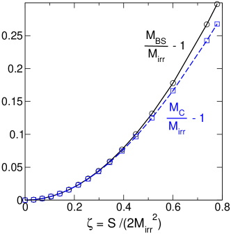
Figure 1: Single spinning unboosted centered black hole: The ratio of the Bondi-Sachs mass ($M_{\rm BS}$) to the irreducible mass ($M_{\text{irr}}$) is compared to the ratio of the Christodoulou mass ($M_{\rm C}$) to the irreducible mass, as the spin extremality parameter $\zeta$ is varied from $0$ to $0.78$.

IV.2 Single displaced black hole with zero spin and boost

Now we displace a single, non-spinning, unboosted black hole a coordinate distance $D$ (in the $x$-direction) from the center of the $\dot{\mathscr{I}^{+}}$ coordinate sphere. The other Bowen-York parameters are the same as for our representative spherically symmetric black hole. Surprisingly, rather than being zero, the velocity of the black hole in the asymptotic Minkowski frame (given by the ratio of the Bondi-Sachs momentum to the Bondi-Sachs energy) is proportional to and in the same direction as the displacement from the origin, as shown in Fig. 2. The dominant contributions to the Bondi-Sachs energy and momentum are from the conformal factor, and have opposite signs from the contributions associated directly with the extrinsic curvature. The contributions from the extrinsic curvature, as calculated using Eqs. (56) and (58), are simply $(E_{\rm BS})_{\rm K}=-KC/3$ and $(\mathbf{P}_{\rm BS})_{\rm K}=-(\mathbf{D}/R_{+})KC/3$. With $\bar{D}=0.1$, $\bar{M}_{\rm irr}=0.028340$, and $\bar{C}=0.0011207$, the fractional extrinsic curvature contributions to the Bondi-Sachs energy and momentum are, respectively, $(E_{\rm BS})_{\rm K}/E_{\rm BS}=-0.039$ and $(\mathbf{P}_{\rm BS})_{\rm K}/\mathbf{P}_{\rm BS}=-0.019$.

Figure 2: Single black hole displaced in the $x$-direction with no boost or spin. The velocity of the black hole in the asymptotic Minkowski frame, $|P^{x}_{\rm BS}|/E_{\rm BS}$, is plotted against the relative displacement $\bar{D}^{x}=D^{x}/R_{+}$. The remaining input parameters ($\bar{C}$, $\bar{R}_{\rm ms}$) have their usual values.

As an indication of whether the displaced black hole is just a moving Schwarzschild black hole or whether it has additional distortions, we compare the Bondi-Sachs mass as given by Eq. (53) with the irreducible mass derived from the area of the apparent horizon. We find that these are the same to the numerical accuracy of our calculations (about $5$ significant figures), which suggests that the displaced black hole is in fact just a Schwarzschild black hole in an asymptotic Lorentz frame in which the black hole is not at rest. We have not tried to prove this more decisively, by finding the coordinate transformation to the conventional form of the Schwarzschild metric.

IV.3 Single centered boosted black hole

Now consider a Bowen-York boost as the only deviation from Schwarzschild. On an asymptotically flat hypersurface, such as a maximal hypersurface, the Bowen-York boost is equal to the physical ADM momentum. In the limit of small $K^{2}C$, there is a range of $R$ over which $\Omega$ is roughly constant near its maximum and $M_{\rm irr}<<R/\Omega<<1/K$, a region of the CMC hypersurface approximating the asymptotic part of a maximal hypersurface. Ref. [1] argued on this basis for using $\mathbf{P}\,\Omega_{\rm max}$ as an estimate of the Bondi-Sachs linear momentum. The close agreement between $\bar{P}^{z}$ and $(K/3)P_{\rm BS}^{z}$ in Table 1 shows that over the entire range of boosts considered, $(KR_{+}/6)P^{z}$ is within about one percent of $P_{\rm BS}^{z}$. The ratio of the actual numerical result for $\Omega_{\rm max}$ to the $KR_{+}/6$ analytic estimate varies from $0.931$ to $0.858$ over this range, so it is considerably better to use the analytic estimate for $\Omega_{\rm max}$, rather than its actual numerical value, in relating the Bowen-York boost to the physical momentum of a centered black hole.

The fact that $M_{\rm BS}/M_{\rm irr}$ becomes significantly larger than $1$ as the black hole motion becomes relativistic shows that the boosted Bowen-York black holes are definitely not simply Schwarzschild black holes moving relative to the asymptotic Minkowski frame. There is additional energy associated with non-kinematic distortions of the geometry. From Eq. (56), we see that for centered black holes, the direct contribution to the Bondi-Sachs energy from the conformal extrinsic curvature is independent of the boost, and for the initial data calculated here, $(E_{\rm BS})_{\rm K}/M_{\rm irr}\approx-0.04$, which is small compared with the positive contribution from conformal factor. In contrast, the the Bondi-Sachs momentum is strongly dominated by the contribution from the conformal extrinsic curvature for centered black holes, since by Eq. (58), $(\mathbf{P}_{\rm BS})_{\rm K}=(3/K)\bar{\mathbf{P}}$.

The $Q^{i}$ boosts are taken to be zero rather than the inversion-symmetric values often assumed in Bowen-York initial value calculations on maximal hypersurfaces (e.g., in Ref. [25]). Only one side of the Einstein-Rosen bridge is astrophysically relevant, since the other side cannot exert any causal influence on the astrophysical side. There is no very compelling reason, other than geometrical elegance, to assume any symmetry between the two sides of the bridge or that the bridges of multiple black holes connect to a common asymptotically flat space. The geometry of the physical space in the immediate vicinity of the black holes may depend to some extent on whether the $Q^{i}$ are zero or inversion symmetric, with possible small effects on the results for the Bondi energy and momentum, but such effects should not be noticeable for the near trumpet considered here, and disappear completely in the limit of an extreme trumpet configuration $(R_{\rm ms}\to 0)$.

$\bar{P}^{z}\times 10$	0.0	0.13889	0.27778	0.55556	0.83333	1.11111	1.38889
$(K/3)P_{\rm BS}^{z}\times 10$	0.0	0.13641	0.27352	0.54974	0.82708	1.10474	1.38249
$(K/3)M_{\rm irr}\times 10$	0.28339	0.28334	0.28338	0.28361	0.28382	0.28390	0.28388
$P_{\rm BS}^{z}/M_{\rm irr}$	0.0	0.48142	0.96521	1.93839	2.91413	3.89129	4.87005
$E_{\rm BS}/M_{\rm irr}$	1.0	1.11221	1.41439	2.32632	3.39577	4.52196	5.67844
$M_{\rm BS}/M_{\rm irr}$	1.0	1.00261	1.03387	1.28624	1.74330	2.30348	2.92016

Table 1: Centered black hole with varying Bowen-York boost $\bar{P}^{z}$. The $\bar{C}$ parameter is fixed at our adopted standard value, and $R_{\rm ms}/R_{+}$ is adjusted to keep the irreducible mass roughly constant as $\bar{P}^{z}$ increases. The input and output quantities are tabulated in the dimensionless and conformal-scale invariant forms discussed earlier in Section IV.

For a slightly different slant on our results, we plot in Fig. 3 (i) the fractional “excess mass” of the black hole $M_{\rm BS}/M_{\text{irr}}-1$, (ii) the velocity of the black hole $v^{z}\equiv P^{z}_{\rm BS}/E_{\rm BS}$ in the asymptotic Minkowski frame, and (iii) the similar excess ADM mass for a boosted Bowen-York black hole on a maximal hypersurface, all as functions of the ratio of the appropriate physical momentum (Bondi-Sachs or ADM) to the irreducible mass. Data for the last curve are taken from Table II of Ref. [25], for $C=0$ and inversion-symmetric $Q^{i}$. Note that as the boost and physical momentum increase, the gravitational mass $M_{\rm BS}$ (solid black curve) increases rapidly enough that the black hole’s velocity $v^{z}\equiv P^{z}_{\rm BS}/E_{\rm BS}$ (violet dash-dot curve) asymptotes to a value less than one (about $0.86$). The results of Ref. [25] are quite similar, but with a slightly higher asymptotic velocity. The excess gravitational mass can be thought of as energy stored in distortions of the geometry relative to a boosted Schwarzschild black hole, energy which would be radiated into the black hole and to infinity during subsequent evolution.

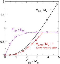
Figure 3: Centered black hole with Bowen-York boosts. Using data from Table 1 above and Table II of Cook and York [25], we plot (i) the fractional excess of the Bondi-Sachs mass over the irreducible mass (solid black line), (ii) the corresponding excess ADM mass of Bowen-York initial data on maximal hypersurfaces (dashed red curve), and (iii) the velocity of the black hole $v^{z}=P^{z}_{\rm BS}/E_{\rm BS}$ (dash-dot violet line) in our initial data. All quantities are shown as a function of the ratio of physical momentum, $P_{\rm BS}$ or $P_{\rm ADM}$ as appropriate, to the irreducible mass. The curves are interpolations between results for discrete models.

The black holes on CMC hypersurfaces have more excess mass than the corresponding black holes on maximal hypersurfaces, modestly so as long as the motion of the black holes is non-relativistic, but more substantially as the motion becomes relativistic. The Cook and York initial data has $C=0$, which in the case of spherical symmetry means that their maximal slice passes through the intersection of the future and past Schwarzschild event horizons, as opposed to the more trumpet-like configurations chosen here and emphasized in Ref. [1]. How much effect this has on the difference in behavior needs further calculations to sort out.

IV.4 Displaced and boosted black holes

In this section, we lay the groundwork for building a binary black hole initial data set on CMC hypersurfaces. For binary black holes in circular orbit, we want each black hole considered by itself to have zero radial momentum and transverse momentum corresponding to that of a mass in a circular orbit, which can be estimated crudely from the Newtonian equations of motion. Since we have seen that a displaced unboosted black hole on a CMC slice has a non-zero radial momentum, this requires finding the radial boost which makes the net Bondi-Sachs momentum of a displaced single black hole zero, and then the transverse boost which generates the desired transverse physical momentum. Once this is done for each black hole of the binary considered separately, the Bowen-York data for the black holes can be superimposed and the Bondi-Sachs energy and momentum of the full system calculated. As long as the two black holes are well-separated, we should find that the Bondi-Sachs energy of the combined system is less than the sum of the energies of the black holes considered separately by something close to the Newtonian binding energy of the system, provided that the total Bondi-Sachs momentum of the system is close to zero.

The first step is to construct a single black hole which is displaced from the center of the coordinate grid and at rest. Fig. 4 shows that this result can be achieved by giving the black hole an appropriate boost antiparallel to its displacement. For the example shown in Fig. 4, the hole is displaced in the positive x-direction, with $\bar{D}^{x}=0.1$. A rescaled boost $\bar{P}^{x}=-0.006$ very nearly cancels the radial momentum associated with the displacement, yielding a net $P^{x}_{\rm BS}/M_{\text{irr}}=-9.6\times 10^{-6}$.

Figure 4: Finding the Bowen-York boost that cancels the Bondi-Sachs momentum associated with the displacement $\bar{D}^{x}=0.1$. The CMC parameters have their usual values, except that $\bar{R}_{\rm ms}$ is varied with the boost to keep $\bar{M}_{\rm irr}$ approximately constant.

Next, we build an initial data set with two non-spinning displaced black holes, each of which considered separately has zero Bondi-Sachs momentum, and calculate the gravitational binding energy; i.e., the decrease in the Bondi-Sachs energy of the combined system compared with the sum of Bondi-Sachs energies of each hole separately. The input parameters are chosen so that, as estimated by the procedures outlined in Sec. IIID of [1] for Schwarzschild black holes, the ratio of minimal surface radius to horizon radius for each hole is about $0.8$, the ratio of the black hole masses $M^{\rm A}/M^{\rm B}\approx 2/1$, and the total rescaled irreducible mass of the system is about $0.7$ that of our standard single black hole. We locate holes A and B along the x-axis at $\bar{D}^{x}_{\rm A}=0.04$ and $\bar{D}^{x}_{\rm B}=-0.08$, so the center of mass of the system is close to the origin. The values for $\bar{C}^{A}$ and $\bar{C}^{B}$ are, respectively, $0.000228$ and $0.0000568$. The scaled minimal surface radii are $\bar{R}_{\rm ms}^{\rm A}=0.000978$ and $\bar{R}_{\rm ms}^{\rm B}=0.000489$. We apply Bowen-York boosts which for each black hole in isolation approximately cancel the Bondi-Sachs radial momentum due to that hole’s displacement. The dimensionless Bondi-Sachs masses ($\bar{M}_{\rm BS}\equiv(K/3)M_{\rm BS}$) for each hole in isolation are $\bar{M}_{\rm BS}^{A}=0.013104$ and $\bar{M}_{\rm BS}^{B}=0.006604$. When the black holes are superimposed, we find that the combined Bondi-Sachs momentum is less than the sum of the already small values for the individual holes. The dimensionless Bondi-Sachs mass of the superimposed black holes is $\bar{M}_{\rm BS}=0.019368$, which is $0.000340$ less than the sum of the individual values. The Newtonian gravitational binding energy of the system is $U=M^{\rm A}M^{\rm B}/{r_{\rm AB}}\approx\Omega_{\rm max}M^{\rm A}M^{\rm B}/|\mathbf{D}^{A}-\mathbf{D}^{B}|$ or, using the analytic estimate of $\Omega_{\rm max}$, $KU/3\approx 0.5R_{+}\;\bar{M}_{\rm BS}^{\rm A}\;\bar{M}_{\rm BS}^{\rm B}/|\bar{\mathbf{D}}^{A}-\bar{\mathbf{D}}^{B}|=0.000371$, which is reasonably close to the rescaled general relativistic binding energy.

The third step is to determine how Bowen-York boosts transverse to a black hole’s displacement translate into the transverse motion of the black hole as revealed by its physical transverse momentum. We have calculated the Bondi-Sachs energy, linear momentum, and angular momentum of a displaced black hole with nearly zero radial momentum and various transverse boosts. The relationship between transverse boost and transverse physical momentum is very close to what we found between boost and momentum for a centered black hole in Sec. IV.3. An example of the comparison for a black hole given a moderately relativistic Bowen-York boost transverse to the displacement in the $x$-direction is given in Table 2. We conclude that it is acceptable to use the results for a centered boosted black hole in Sec. IV.3, including the analytic formula, when estimating the transverse Bowen-York boosts appropriate for black holes in quasi-circular binary orbits. Of course, the displaced black holes also acquire orbital angular momentum according to Eq. (50).

$\bar{D}^{x}$	$\bar{P}^{y}\times 10$	$(K/3)M_{\text{irr}}\times 10$	$P_{\rm BS}^{y}/M_{\text{irr}}$	$E_{\rm BS}/M_{\text{irr}}$	$M_{\rm BS}/M_{\text{irr}}$	$J^{z}/M_{\text{irr}}^{2}$
0	0.13889	0.28334	0.48142	1.11220	1.00261	0
0.1	0.13889	0.28336	0.47686	1.11117	1.00365	3.45956

Table 2: A centered black hole (first row) and a displaced black hole (second row) are both given the same mildly relativistic (transverse) rescaled Bowen-York boosts $\bar{P}^{y}=0.013889$. The displaced black hole is also given a longitudinal rescaled boost $\bar{P}^{x}=-0.00660$ to approximately cancel the physical momentum associated with the displacement. The other input parameters for both holes have the standard values. The black holes have almost identical physical properties, except for the orbital angular momentum of the displaced hole.

The close relationship between the transverse Bondi-Sachs momentum and the transverse rescaled Bowen-York boost can be understood as a consequence of the dominance of the direct contribution to the Bondi-Sachs momentum from the conformal extrinsic curvature, as calculated in Eq. (58), over the contribution from the conformal factor for these transverse components. As long as $\bar{D}$ is reasonably small, the dominant transverse term in Eq. (58) is just $(KR_{+}/6)P_{\rm trans}$. There is no simple relation between the longitudinal component of the Bondi-Sachs momentum and the longitudinal component of the Bowen-York boost because the conformal factor contribution to the longitudinal component is not small.

IV.5 Binary black hole initial data

Here we build on the results of the previous subsections to construct initial data for two spinning unequal-mass black holes with initial momenta roughly appropriate for circular orbits. The input parameters are chosen based on a Newtonian analysis, in circumstances such that the post-Newtonian corrections are roughly at the $10\%$ level. Ignoring relativistic corrections is consistent with other sources of uncertainty, such as estimating parameters for each black hole in isolation, ignoring their tidal interactions. While similar initial data were presented in [1], we are now on much firmer ground in considering the relationship between the Bowen-York parameters and the physical properties of each hole.

We consider two examples. Both are constructed to have about a 2:1 mass ratio and roughly a 12:1 ratio of physical distance between the black holes to the total gravitational mass of the system. The minimal surface radii are chosen to give moderately trumpet-like configurations. The black holes are assigned close to maximal spins oriented in the orbital plane and perpendicular to the displacement between the holes. In one case (Case I), the ratio of coordinate separation of the holes to the coordinate radius of $\mathscr{I}^{+}$ is $0.12$, and in the other case (Case II), it is three times larger. In the latter case, there is the potential for greater computational efficiency, since the black holes can be resolved with a lower resolution grid.

The Newtonian analysis of a circular orbit binary system with masses $M_{\rm A}$ and $M_{\rm B}$ separated by a distance $r_{\rm AB}$ gives for the equal and opposite momenta of the masses

$$P_{\rm A}^{y}=-P_{\rm B}^{y}=\frac{M_{\rm A}M_{\rm B}}{M_{\rm A}+M_{\rm B}}\sqrt{\frac{M_{\rm A}+M_{\rm B}}{r_{\rm AB}}},$$

perpendicular to the displacements of the black holes (which are along the $x$-axis). Equating the transverse rescaled Bowen-York boost to $K/3$ times the transverse physical momentum, for $M_{\rm A}\approx 2M_{\rm B}$, we choose $\bar{P}^{y}=0.064(K/3)(M_{\rm A}+M_{\rm B})$, since $r_{\rm AB}$ is about $12$ times the total mass. Estimating black hole masses from the Bowen-York parameters is a bit uncertain when the black holes are not Schwarzschild, but consistency with the total system mass can be verified retrospectively.

The non-zero input parameters chosen for Case I are $\bar{C}_{\rm A}=2.4531\times 10^{-5}$, $\bar{C}_{\rm B}=5.1224\times 10^{-6}$, $\bar{S}_{\rm A}^{y}=6.5224$, $\bar{S}_{\rm B}^{y}=-7.8088$, $\bar{D}_{\rm A}^{x}=0.04$, $\bar{D}_{\rm B}^{x}=-0.08$, $\bar{R}_{\rm ms}^{\rm A}=9.78\times 10^{-4}$, $\bar{R}_{\rm ms}^{\rm B}=4.89\times 10^{-4}$, and boost components $\bar{P}_{\rm A}^{x}=-0.001074$, $\bar{P}_{\rm A}^{y}=0.00116$, $\bar{P}_{\rm B}^{x}=0.001060$, $\bar{P}_{\rm B}^{y}=-0.00116$. As noted in Sec. IV.1, we expect the rescaled black hole masses to scale roughly as $\bar{C}_{\rm eff}=\left[\bar{C}\sqrt{1+2\left(\bar{S}\right)^{2}}\right]^{1/2}$, which is $0.0150864$ for hole A and $0.0075366$ for hole B. The large values of $\bar{S}$ for each hole mean that the black holes have close to the maximum possible spin extremality parameter $\zeta$.

In Case II, the input parameters are $\bar{C}_{\rm A}=3.6231\times 10^{-4}$, $\bar{C}_{\rm B}=8.5343\times 10^{-5}$, $\bar{S}_{\rm A}^{y}=3.9347$, $\bar{S}_{\rm B}^{y}=-4.1761$, $\bar{D}_{\rm A}^{x}=0.12$, $\bar{D}_{\rm B}^{x}=-0.24$, $\bar{R}_{\rm ms}^{\rm A}=2.934\times 10^{-3}$, $\bar{R}_{\rm ms}^{\rm B}=1.467\times 10^{-3}$, and boost components $\bar{P}_{\rm A}^{x}=-0.010026$, $\bar{P}_{\rm A}^{y}=0.00348$, $\bar{P}_{\rm B}^{x}=0.010617$, $\bar{P}_{\rm B}^{y}=-0.003639$. The $\bar{C}_{\rm eff}$ values are $0.04526$ for hole A and $0.02261$ for hole B, about three times the values in Case I, while the $\bar{D}$ values are also three times larger. This suggests the two cases are similar in the ratio of physical separation of the holes to the total mass of the system. The $\bar{S}$ values are smaller in Case II than in Case I; this is because the elliptic solver failed to converge if we tried to make the $\bar{S}$ values as large as in Case I. Another effect of the larger ratio of the size of the binary system to $3/K$ in Case II is the larger $\bar{P}^{x}$ values needed to cancel out the radial components of the individual black hole momenta.

Our results for the irreducible masses and angular momenta of the individual holes and the physical energy, momentum, mass, and angular momentum of the systems are given in Table 3. Note that there are non-zero, though small, $z$-components for the system velocities even though none of the boosts has a non-zero $z$-component. This is the result of the spins of the black holes interacting with the geometry of the hypersurface, one indication of which is the $\mathbf{D}\times\mathbf{S}$ term in Eq. (58). Also, note that $K/3=0.02$ gives a total system mass close to $1$ in Case I, and this together with $R_{+}=100$ makes coordinate distances close to physical distances. The same is true for Case II since $K$ is increased and $R_{+}$ is decreased by a factor of $3$. The calculations for Case II took about $80\%$ of the time on the same computer as the calculations for Case I, indicating some potential for realizing increased efficiency of computation by having the binary system occupy a larger fraction of the conformal domain.

	$\bar{M}_{\rm irr}$	$(K/3)E_{\rm BS}$	$(K/3)M_{\rm BS}$	$P_{\rm BS}^{x}/E_{\rm BS}$	$P_{\rm BS}^{y}/E_{\rm BS}$	$P_{\rm BS}^{z}/E_{\rm BS}$	$(K/3)^{2}J^{x}$	$(K/3)^{2}J^{y}$	$(K/3)^{2}J^{z}$
	$\times 10^{2}$	$\times 10^{2}$	$\times 10^{2}$	$\times 10^{3}$	$\times 10^{3}$	$\times 10^{3}$	$\times 10^{4}$	$\times 10^{4}$	$\times 10^{4}$
Case I
hole A:	1.06367	n/a	n/a	n/a	n/a	n/a	0	1.60000	0.92800
hole B:	0.53449	n/a	n/a	n/a	n/a	n/a	0	-0.40000	1.85600
system:	1.59816	1.96685	1.96685	-1.04379	0.25464	0.05850	0	1.20000	2.78400
Case II
hole A:	3.16247	n/a	n/a	n/a	n/a	n/a	0	14.25600	8.35200
hole B:	1.62032	n/a	n/a	n/a	n/a	n/a	0	-3.56400	17.46720
system:	4.78280	5.90011	5.90003	-5.25838	-0.16546	0.17739	0	10.69200	25.81920

Table 3: Physical quantities for two binary black hole initial data sets. (See text for input parameter values.) From left to right are the irreducible masses, the Bondi-Sachs energy, the Bondi-Sachs mass, the system velocity components, and the angular momentum components, all made dimensionless by appropriate powers of $K/3$. There are no well-defined Bondi-Sachs energy and linear momentum for the individual black holes, but the angular momenta can be calculated using Eq. (65).

While the system momentum and velocity should ideally be zero, this is not precisely the case in our calculations, which made no attempt to fine-tune the input parameters. Still, the residual system velocities are quite small compared with the Newtonian estimates for the orbital velocities. The system mass is significantly greater than the sum of the irreducible masses in both Cases I and Case II, since the contributions of the spins to the black hole hole masses dominates over their gravitational binding energy. The slightly smaller spins in Case II make this effect somewhat smaller there. Of course, the system mass can never be less than the total irreducible mass.

V Discussion

The first part of this paper is a discussion of the asymptotic behavior of the conformal factor $\Omega$, the conformal spatial metric, and the conformal extrinsic curvature of CMC hypersurfaces in the neighborhood of $\mathscr{I}^{+}$ as constrained by the initial value equations for astrophysically general asymptotically flat spacetimes, and a calculation of the Bondi-Sachs mass aspect in terms of the coefficients in the expansion away from the $\dot{\mathscr{I}^{+}}$ 2-surface, which is the intersection of the CMC hypersurface with the $\mathscr{I}^{+}$ null hypersurface. In this analysis, we adopt special spatial coordinates, Gaussian normal coordinates based on $\dot{\mathscr{I}^{+}}$, and use the conformal proper distance $z$ from $\dot{\mathscr{I}^{+}}$ along the normal spatial geodesics as the expansion parameter. Angular coordinates are propagated along the normal spatial geodesics, initialized to be standard polar coordinates on $\dot{\mathscr{I}^{+}}$, which is assumed to be a true sphere with intrinsic curvature $\xi_{0}^{2}$. This is not a physical constraint for an asymptotically flat spacetime with a topologically spherical null infinity, just a constraint on the conformal gauge. The asymptotic expansion is essentially identical to that presented in Ref. [9], except we do not allow the polyhomogeneous terms in the expansion of the angular part of the conformal spatial metric through $O(z^{2})$ that are a major focus of that paper. No such terms are present unless they are present at some arbitrarily early time, which means that they should be associated with incoming radiation at past null infinity. In typical astrophysical problems incoming radiation near $\mathscr{I}^{+}$ should only be generated by backscatter or nonlinear interaction of outgoing radiation, and should not be present ab initio, except for what might be plausibly associated with backscatter of radiation emitted before the start of the numerical calculation.

As noted in Ref. [9], polyhomogeneous terms are nevertheless generically present at $O(z^{4})$ in the expansion of the conformal factor and at $O(z^{2})$ in the expansion of the conformal extrinsic curvature. The authors of Ref. [9] considered the vanishing of the expression in Eq. (39) a condition for the absence of these polyhomogeneous terms, but we point out that the condition cannot be satisfied over any finite time interval in which outgoing gravitational radiation, as indicated by time variation of $\breve{\chi}_{\rm AB}$, is present at $\mathscr{I}^{+}$ (see also Ref. [8]). The implied smoothness of only $C^{3}$ for the conformal factor and $C^{1}$ for the conformal extrinsic curvature at $\mathscr{I}^{+}$ is a gauge artifact of the CMC hypersurface condition. The offending terms are not present if the physical mean curvature $K$ has precisely the right angular dependence at $O(z^{3})$ in a power series expansion away from $\dot{\mathscr{I}^{+}}$. This cannot be accomplished by any predetermined specification of $K$, but maintaining a high degree of smoothness at $\mathscr{I}^{+}$ is possible with fully hyperbolic evolution schemes, such as the regular conformal field equations of Friedrich [26, 27], as well as with the Bondi-Sachs gauge.

For the assumed special geometric properties of $\dot{\mathscr{I}^{+}}$ to be preserved during evolution, a constraint must be placed on the evolution of the conformal factor; specifically, that the trace of the conformal extrinsic curvature $\tilde{K}$ satisfy the boundary condition of Eq. (17). This says that the 3D mean conformal extrinsic curvature of the CMC hypersurface at $\dot{\mathscr{I}^{+}}$, which governs the evolution of the conformal factor, should equal the 2D mean extrinsic curvature of the $\dot{\mathscr{I}^{+}}$ 2-surface when both are renormalized according to their respective number of dimensions. All this also assumes preservation of the coordinate location of $\mathscr{I}^{+}$ as a coordinate sphere centered at the origin and propagation of the angular coordinates on $\mathscr{I}^{+}$ along its null generators, which imposes boundary conditions on the shift vector. These boundary conditions can be implemented in a mixed hyperbolic-elliptic evolution scheme like those of Ref. [5] or Ref. [8]. Also, we impose the usual regularity conditions at $\mathscr{I}^{+}$, the “zero-shear” condition and the vanishing of the Weyl tensor, which as shown for the evolution schemes of [5, 8], are preserved by the evolution equations.

We have applied this asymptotic analysis to derive the expression for the Bondi-Sachs mass aspect given in Eq. (38), from which the Bondi-Sachs energy and momentum can be calculated as appropriate angular averages over $\dot{\mathscr{I}^{+}}$. This is a 3D expression, involving only quantities evaluated on a single CMC hypersurface. The 3D expression derived in Section 5.3 of Ref. [17] requires knowledge of a “background” metric and extrinsic curvature in addition to the actual metric and extrinsic curvature of the CMC hypersurface. It is non-trivial to determine the appropriate background quantities. The terms appearing in Eq. (38) are simply related to the asymptotic behavior of the conformal factor, conformal metric, and conformal extrinsic curvature in Gaussian normal coordinates, and can be determined by solving the geodesic equation for the geodesics normal to $\dot{\mathscr{I}^{+}}$ in the CMC hypersurface in any computational spatial gauge satisfying our boundary conditions. The alternative expression of Eq. (40) based on the Weyl tensor is completely equivalent, as can be seen by evaluating the Weyl tensor in the form of Eq. (41) in Gaussian normal coordinates.

With conformally flat initial data, all of this simplifies drastically. With $\dot{\mathscr{I}^{+}}$ a coordinate sphere of constant radius in a flat conformal geometry, the normal geodesics are radial, and the 2D extrinsic curvature of surfaces of constant coordinate radius $R$ is just $R^{-1}$ times the unit sphere metric. The momentum constraint equation admits solutions identical in form to the Bowen-York solutions. We have shown in the Appendices how to evaluate analytically the angular integrals of the term coming from the conformal extrinsic curvature in the mass aspect in terms of the Bowen-York parameters. The only numerical calculation necessary is solving the Hamiltonian constraint equation for the conformal factor and fitting to a power series expansion in the coordinate distance from $\dot{\mathscr{I}^{+}}$, taking advantage of the known analytic form through order $z^{5}$. We have computed how the Bondi-Sachs energy-momentum and the angular momentum of the system depend on the Bowen-York parameters for a sampling of single and double black hole systems, similar to those considered in Ref. [1].

For a single black hole centered at the origin, with varying Bowen-York spin (which in this case equals the system angular momentum), the results are displayed in Fig. 1. They show that the “rotational energy” of the black hole, the excess of the Bondi-Sachs mass over the irreducible mass, has a dependence on the spin extremality parameter $\zeta$ similar to that of Kerr black holes. The Bondi-Sachs mass is a bit larger in our case, as one would expect. The main difference is that our sequence cannot be extended to as large a value of the extremality parameter as the Kerr sequence.

A single non-spinning, unboosted black hole displaced from the origin, i.e., displaced relative to the center of the sphere representing future null infinity, is more interesting. As shown in Fig. 2, the displaced black hole acquires a velocity in the asymptotic Minkowski frame in the direction of its displacement close to twice the ratio of the displacement to $R_{+}$. Consequently, when constructing initial data for black hole binaries on CMC hypersurfaces, compensating Bowen-York boosts directed inward should be introduced for each displaced black hole, so that its net radial velocity is zero.

Results for a single centered black hole given various, mostly rather large, boosts are presented in Sec. IV.2. Here we emphasize how close the numerical result for the Bondi-Sachs momentum $\mathbf{P}_{\rm BS}$ is to $KR_{+}/6$ times the Bowen-York boost vector, even when the black hole is moving at relativistic speeds. Ref. [1], presented a crude hand-waving argument that the physical momentum should be roughly $\Omega_{\rm max}$ (calculated numerically) times the boost. The expected accuracy of this estimate was of order $KM_{\rm irr}$, or about $10\%$ for our choices of Bowen-York parameters. Comparison of the first two rows of Table 1 shows that $KR_{+}/6$ times the boost is within about $1\%$ of $\mathbf{P}_{\rm BS}$, while $KR_{+}/6$ differs from $\Omega_{\rm max}$ by about $10\%$. The physical properties of these boosted centered black holes are explored further in Fig. 3 and compared with corresponding results for boosted black holes on maximal hypersurfaces. In both cases, the ratio of physical mass to irreducible mass increases rather rapidly with increasing boost, and the velocity of the black hole plateaus at a value somewhat less than the speed of light for large boosts. Bowen-York initial data cannot produce black holes moving at speeds arbitrarily close to the speed of light.

A combination of boosts and displacements is necessary to construct initial data for binary black holes. In Section IV.4, we first determine the radial boost opposite to the direction of the displacement necessary to cancel the radial momentum induced by the displacement. Orbital motion of a black hole in a binary system requires a transverse boost, and we verified in Table 2 that the relationship between the transverse boost and transverse momentum for a displaced black hole is very nearly the same as the relation between boost and momentum for a centered boosted black hole, as calculated in Section IV.2. We also checked that the gravitational binding energy of two black holes at rest separated by about 10 times the total gravitational mass of the system agrees reasonably well with the Newtonian formula.

Finally, we make a crude attempt to construct initial data for two black holes in circular orbits about the center of mass. Again, the black holes, with about a 2:1 mass ratio, are separated by a proper distance about 10 times the gravitational mass of the system. Boosts are assigned so that, considered individually, each black hole has zero radial momentum and transverse momentum roughly as expected from a Newtonian analysis of the orbit. The black holes are also given close to maximal spins oriented in the plane of the orbit. The total energy, momentum, and angular momentum of the system are calculated and displayed in Table 3. The numerical results are consistent with the system linear momentum being close to zero, in that the system $P^{i}_{\rm BS}/E_{\rm BS}$ values are rather small compared to the $\bar{P}^{i}/\bar{M}_{\rm irr}$ for each black hole. The component of the residual momentum along the line of the black hole displacements (the $x$-component) is considerably larger than the other components, suggesting that we should have taken account of the black hole spins in estimating the radial boosts. The system angular momentum, including both spin and orbital angular momentum, is roughly consistent with Newtonian expectations. The two cases we present are designed to have similar ratios of physical separation to black hole masses, but values of $(K/3)M_{\rm BS}$ differing by about a factor of three. The ratio of the coordinate separation of the holes to $R_{+}$ is three times larger in Case II than in Case I, implying correspondingly larger effects of the warping of the CMC hypersurface at the scale of the binary system. Nonetheless, Case II achieves close to the same accuracy as Case I with half the number of collocation points in the outer spherical computational domain surrounding the two holes, $40$ versus $80$.

The exploratory analyses of conformally flat initial data on CMC hypersurfaces carried out in Ref. [1] and this paper need to be extended in various ways to approach the current sophistication of initial data calculations on maximal hypersurfaces. In particular, it would be interesting to see how well the numerical techniques used here hold up when considering non-conformally-flat data, particularly when radiation is present at $\dot{\mathscr{I}^{+}}$. How well does the SpEC elliptic solver handle the more complicated asymptotic behavior, including the polyhomogeneous terms in the conformal factor and extrinsic curvature? This is important for implementing mixed hyperbolic-elliptic evolution systems. Also, quasi-equilibrium methods [28, 29, 30] based on the conformal-thin-sandwich approach to the initial data problem [31, 32] have come to the fore in recent years as a way of obtaining quieter starts to binary black hole calculations, with less junk radiation and more circular initial orbits. It is clearly worthwhile to attempt to adapt these approaches to initial data on CMC hypersurfaces. Can initial data for more Kerr-like black holes, as in Ref. [33], be constructed on CMC hypersurfaces? We hope to explore such issues in future papers.

Appendix A Analytic calculation of the partial Bondi-Sachs four-momentum from the conformal extrinsic curvature

The Bondi-Sachs mass aspect for the conformally flat initial data is given in Eq. (46) as the sum of two terms, one a coefficient in the expansion of the conformal factor away from $\dot{\mathscr{I}^{+}}$, and the other a projection $\bar{A}_{RR}$ of the conformal extrinsic curvature defined by Eq. (45). The first term requires solving a non-linear elliptic equation, which can only be done numerically. However, in the case of Bowen-York initial data on a conformally flat spatial geometry, the conformal extrinsic curvature $\tilde{A}_{ij}$ is as given explicitly in Eq. (42). The angular integrals on $\dot{\mathscr{I}^{+}}$ for the $\bar{A}_{RR}$ contribution to the Bondi-Sachs mass and linear momentum will be obtained in analytic form with the help of Mathematica.

For a given black hole, we can rotate the Cartesian coordinates in the conformal flat space to locate the black hole on the polar (positive $z$-) axis. The unit vector $\mathbf{N}$ normal to $\dot{\mathscr{I}^{+}}$ has Cartesian components $N^{i}=\left({\sin\theta\cos\phi,\,\sin\theta\sin\phi,\,\cos\theta}\right)$. The displacement from the black hole location to a point on $\dot{\mathscr{I}^{+}}$ has components

$$r^{i}=\left({R_{+}\sin\theta\cos\phi,\,R_{+}\sin\theta\sin\phi,\,R_{+}\cos\theta-D}\right)\equiv rn^{i},$$

where $\mathbf{n}$ is a unit vector. With $q\equiv D/R_{+}$ and $x\equiv\cos\theta$, the coordinate distance from the black hole to the point on $\dot{\mathscr{I}^{+}}$ is

$$r=R_{+}\sqrt{1+q^{2}-2qx}.$$

The scalar and vector products of the two unit vectors are

$$\mathbf{N}\cdot\mathbf{n}=\frac{{1-qx}}{{\sqrt{1+q^{2}-2qx}}},\,\,\,\,\,\,\mathbf{N}\times\mathbf{n}=\frac{{q\sin\theta}}{{\sqrt{1+q^{2}-2qx}}}\left({-\sin\phi,\,\cos\phi,\,0}\right).$$

The direct contribution to the Bondi-Sachs mass aspect $M_{\rm A}$ from the conformal extrinsic curvature is

$$\left({M_{{{\rm A}}}}\right)_{{\rm K}}=-\frac{3}{K}\bar{A}_{RR}=-\frac{K}{6}R_{+}^{3}N^{k}\tilde{A}_{k\ell}N^{\ell}.$$ (55)

Substituting the expression in Eq. (42) gives

$$\left({M_{{{\rm A}}}}\right)_{{\rm K}} = -\frac{{KC}}{6}\left({\frac{R}{r}}\right)^{3}\left[{3\left({\mathbf{N}\cdot\mathbf{n}}\right)^{2}-1}\right]-K\left({\frac{R}{r}}\right)^{3}\mathbf{S}\cdot\left({\mathbf{N}\times\mathbf{n}}\right)\left({\mathbf{N}\cdot\mathbf{n}}\right)$$

$$+\frac{{KR_{+}}}{4}\left({\frac{{R_{+}}}{r}}\right)^{2}\left[{2\left({\mathbf{N}\cdot\mathbf{P}}\right)\left({\mathbf{N}\cdot\mathbf{n}}\right)+\left({\mathbf{n}\cdot\mathbf{P}}\right)\left({\left({\mathbf{N}\cdot\mathbf{n}}\right)^{2}-1}\right)}\right]$$

$$-\frac{K}{{4R_{+}}}\left({\frac{{R_{+}}}{r}}\right)^{4}\left[{2\left({\mathbf{N}\cdot\mathbf{Q}}\right)\left({\mathbf{N}\cdot\mathbf{n}}\right)+\left({\mathbf{n}\cdot\mathbf{Q}}\right)\left({1-5\left({\mathbf{N}\cdot\mathbf{n}}\right)^{2}}\right)}\right].$$

The contribution of this to the Bondi-Sachs energy is the average of Eq. (55) over solid angle. Since the average of any term with an odd power of $\cos\phi$ or $\sin\phi$ vanishes, the spin term and the components of $\mathbf{P}$ and $\mathbf{Q}$ perpendicular to $\mathbf{D}$ do not contribute. We have

$$\left({E_{{{\rm BS}}}}\right)_{{\rm K}} = -\frac{{KC}}{6}\left[{\frac{3}{2}\int\limits_{-1}^{1}{dx\frac{{\left({1-qx}\right)^{2}}}{{\left({1+q^{2}-2qx}\right)^{5/2}}}-\frac{1}{2}\int\limits_{-1}^{1}{\frac{{dx}}{{\left({1+q^{2}-2qx}\right)^{3/2}}}}}}\right]$$

$$+\frac{{KR_{+}}}{4}P^{z}\left[{\int\limits_{-1}^{1}{dx\frac{{x\left({1-qx}\right)}}{{\left({1+q^{2}-2qx}\right)^{3/2}}}+\frac{1}{2}\int\limits_{-1}^{1}{dx\frac{{\left({x-q}\right)\left({1-qx}\right)^{2}}}{{\left({1+q^{2}-2qx}\right)^{5/2}}}-\frac{1}{2}\int\limits_{-1}^{1}{dx\frac{{\left({x-q}\right)}}{{\left({1+q^{2}-2qx}\right)^{3/2}}}}}}}\right]$$

$$-\frac{K}{{4R_{+}}}Q^{z}\left[{\int\limits_{-1}^{1}{dx\frac{{x\left({1-qx}\right)}}{{\left({1+q^{2}-2qx}\right)^{5/2}}}+\frac{1}{2}\int\limits_{-1}^{1}{dx\frac{{\left({x-q}\right)}}{{\left({1+q^{2}-2qx}\right)^{5/2}}}-\frac{5}{2}\int\limits_{-1}^{1}{dx\frac{{\left({x-q}\right)\left({1-qx}\right)^{2}}}{{\left({1+q^{2}-2qx}\right)^{7/2}}}}}}}\right].$$

Evaluating the integrals with Mathematica,

$$\left({E_{{{\rm BS}}}}\right)_{{\rm K}} = -\frac{{KC}}{6}\left[{\frac{{3-2q^{2}}}{{1-q^{2}}}-\frac{1}{{1-q^{2}}}}\right]+\frac{{KR_{+}}}{4}P^{z}\left[{\frac{4}{3}q+0-0}\right]$$

$$-\frac{K}{{4R_{+}}}Q^{z}\left[{\frac{4}{3}\frac{{2q-q^{3}}}{{\left({1-q^{2}}\right)^{2}}}+\frac{2}{3}\frac{q}{{\left({1-q^{2}}\right)^{2}}}-\frac{2}{3}\frac{{5q-2q^{3}}}{{\left({1-q^{2}}\right)^{2}}}}\right],$$

which simplifies to

$$\left({E_{{{\rm BS}}}}\right)_{{\rm K}}=-\frac{{KC}}{3}+\frac{K}{3}\left({\mathbf{D}\cdot\mathbf{P}}\right)=\frac{3}{K}\left[-\bar{C}+2\bar{\mathbf{D}}\cdot\bar{\mathbf{P}}\right].$$ (56)

The Bondi-Sachs momentum $\mathbf{P}_{{{\rm BS}}}$ is the average over solid angle of $M_{{{\rm A}}}\,\mathbf{N}$ . The portion of this directly due to the extrinsic curvature is best calculated separately for the components parallel and perpendicular to the displacement $\mathbf{D}$ of the black hole. The component parallel to $\mathbf{D}$ is obtained simply by inserting a factor of $x=\cos\theta$ into each of the integrals in the above expression for $\left({E_{{{\rm BS}}}}\right)_{{\rm K}}$ . Evaluating the integrals gives

$$\left({P_{{{\rm BS}}}^{z}}\right)_{{\rm K}} = -\frac{{KC}}{6}\left[{\frac{{3q-2q^{3}}}{{1-q^{2}}}-\frac{q}{{1-q^{2}}}}\right]+\frac{{KR_{+}}}{4}P^{z}\left[{\frac{{10+12q^{2}}}{{15}}+\frac{{5-2q^{2}}}{{15}}-\frac{1}{3}}\right]$$

$$-\frac{K}{{4R_{+}}}Q^{z}\left[{\frac{2}{3}\frac{{1+3q^{2}-2q^{4}}}{{\left({1-q^{2}}\right)^{2}}}+\frac{1}{3}\frac{{1+q^{2}}}{{\left({1-q^{2}}\right)^{2}}}-\frac{1}{3}\frac{{5+3q^{2}-2q^{4}}}{{\left({1-q^{2}}\right)^{2}}}}\right],$$

which simplifies to

$$\left({P_{{{\rm BS}}}^{z}}\right)_{{\rm K}}=-\frac{{KC}}{3}\frac{D}{{R_{+}}}+\frac{{KR_{+}}}{6}P^{z}\left({1+\left({\frac{D}{{R_{+}}}}\right)^{2}}\right)+\frac{K}{6R_{+}}Q^{z}.$$ (57)

The perpendicular component has a contribution from the spin term in the extrinsic curvature. For instance, the $x$-component is

$$\left({P_{{{\rm BS}}}^{x}}\right)_{{\rm K}} = \frac{{KR_{+}}}{8}P^{x}\left[{\int\limits_{-1}^{1}{dx\frac{{\left({1-x^{2}}\right)\left({1-qx}\right)}}{{\left({1+q^{2}-2qx}\right)^{3/2}}}+\frac{1}{2}\int\limits_{-1}^{1}{dx\frac{{\left({1-x^{2}}\right)\left({1-qx}\right)^{2}}}{{\left({1+q^{2}-2qx}\right)^{5/2}}}-\frac{1}{2}\int\limits_{-1}^{1}{dx\frac{{\left({1-x^{2}}\right)}}{{\left({1+q^{2}-2qx}\right)^{3/2}}}}}}}\right]$$

$$-\frac{K}{{8R_{+}}}Q^{x}\left[{\int\limits_{-1}^{1}{dx\frac{{\left({1-x^{2}}\right)\left({1-qx}\right)}}{{\left({1+q^{2}-2qx}\right)^{5/2}}}+\frac{1}{2}\int\limits_{-1}^{1}{dx\frac{{\left({1-x^{2}}\right)}}{{\left({1+q^{2}-2qx}\right)^{5/2}}}-\frac{5}{2}\int\limits_{-1}^{1}{dx\frac{{\left({1-x^{2}}\right)\left({1-qx}\right)^{2}}}{{\left({1+q^{2}-2qx}\right)^{7/2}}}}}}}\right]$$

$$-\frac{{KD^{z}S^{y}}}{{4R_{+}}}\int\limits_{-1}^{1}{dx\frac{{\left({1-x^{2}}\right)\left({1-qx}\right)}}{{\left({1+q^{2}-2qx}\right)^{5/2}}}}.$$

Evaluating the integrals gives

$$\left({P_{{{\rm BS}}}^{x}}\right)_{{\rm K}} = \frac{{KR_{+}}}{8}P^{x}\left[{\frac{{20-12q^{2}}}{{15}}+\frac{{10-8q^{2}}}{{15}}-\frac{2}{3}}\right]-\frac{K}{{8R_{+}}}Q^{x}\left[{\frac{4}{3}+\frac{2}{3}\frac{1}{{1-q^{2}}}-\frac{2}{3}\frac{{5-4q^{2}}}{{1-q^{2}}}}\right]-\frac{{KD^{z}S^{y}}}{{3R_{+}}}$$

$$= \frac{{KR_{+}}}{6}P^{x}\left[{1-\left({\frac{D}{{R_{+}}}}\right)^{2}}\right]+\frac{K}{{6R_{+}}}Q^{x}-\frac{{KD^{z}S^{y}}}{{3R_{+}}}.$$

Combine this result with Eq. (57) to get in vector form

$$\left({\mathbf{P}_{{{\rm BS}}}}\right)_{{\rm K}}=\frac{3}{K}\left[-\bar{C}\bar{\mathbf{D}}+\bar{\mathbf{P}}\left(1-\left|\bar{\mathbf{D}}\right|^{2}\right)+2(\bar{\mathbf{D}}\cdot\bar{\mathbf{P}})\bar{\mathbf{D}}+\bar{\mathbf{Q}}+\bar{C}\bar{\mathbf{D}}\times\bar{\mathbf{S}}\right].$$ (58)

The expressions in Eqs. (56) and (58) are only portions of the total Bondi-Sachs energy and momentum, respectively, so nothing can be concluded from these expressions about how the total Bondi-Sachs energy and momentum depend on the Bowen-York parameters. In particular, the total Bondi-Sachs energy is always positive even when the typically dominant first term in Eq. (56) is negative. Also, note that a displaced “Schwarzschild” black hole (with no boosts or spin) has, according to our numerical results, a net linear momentum in the opposite direction from that implied by the first term of Eq. (58).

Appendix B Analytic calculation of total angular momentum

For conformally flat initial data on CMC hypersurfaces, the expression in Eq. (49) for the angular momentum at $\dot{\mathscr{I}^{+}}$ is just an angular integral over the conformal extrinsic curvature $\tilde{A}_{\ell}^{~{}k}$, independent of the conformal factor $\Omega$. The generalized Bowen-York expression for $\tilde{A}_{\ell}^{~{}k}$, as given in Eq. (42), is a simple sum over terms for each black hole, each of which contributes independently to the angular momentum. Therefore, we can consider each black hole and each term separately. For a given black hole, we can rotate the Cartesian coordinates in the conformal flat space to locate the black hole with some displacement $\mathbf{D}$ from the origin to put it on the positive $z$-axis. The unit vector $\mathbf{N}$ normal to this sphere at $R=R_{+}$, the unit vector $\mathbf{n}$ directed away from the black hole, and the coordinate distance $r$ from the black hole to a point on $\dot{\mathscr{I}^{+}}$ are given in Appendix A. Also note Eq. (A3) for the scalar and vector products of $\mathbf{N}$ and $\mathbf{n}$. Define $q\equiv D/{R_{+}}$ and $x\equiv\cos\theta$.

The contribution from the first term in Eq. (42) is

$$-\frac{C}{{8\pi}}\oint{\sin\theta d\theta d\phi\left({\frac{{R_{+}}}{r}}\right)^{3}\left[{3\left({\mathbf{N}\times\mathbf{n}}\right)\left({\mathbf{n}\cdot\mathbf{N}}\right)-\left({\mathbf{N}\times\mathbf{N}}\right)}\right]},$$

which is identically zero since the integrand has only odd powers of $\sin\phi$ and $\cos\phi$.

The “spin” term contribution to the total angular momentum is

$$\mathbf{J}_{S} = \frac{3}{{8\pi}}\oint{\sin\theta d\theta d\phi\left({\frac{{R_{+}}}{r}}\right)^{3}\left[{\mathbf{N}\times\left({\mathbf{S}\times\mathbf{n}}\right)\left({\mathbf{n}\cdot\mathbf{N}}\right)+\mathbf{N}\cdot\left({\mathbf{S}\times\mathbf{n}}\right)\left({\mathbf{N}\times\mathbf{n}}\right)}\right]}$$ (59)

$$= \frac{3}{4}\int\limits_{-1}^{1}{\frac{{dx}}{{\left({1+q^{2}-2qx}\right)^{3/2}}}\left\langle{\left({\mathbf{N}\cdot\mathbf{n}}\right)^{2}\mathbf{S}-\left({\mathbf{N}\cdot\mathbf{S}}\right)\left({\mathbf{n}\cdot\mathbf{N}}\right)\mathbf{n}+\mathbf{N}\cdot\left({\mathbf{S}\times\mathbf{n}}\right)\left({\mathbf{N}\times\mathbf{n}}\right)}\right\rangle_{\phi}}.$$

Consider separately the components of $\mathbf{J}$ along and perpendicular to the displacement of the black hole. The component parallel to $\mathbf{D}$ is

$$J_{S}^{z} = \frac{3}{4}S^{z}\left[{\int\limits_{-1}^{1}{dx\frac{{\left({1-qx}\right)^{2}}}{{\left({1+q^{2}-2qx}\right)^{5/2}}}}-\int\limits_{-1}^{1}{dx\frac{{x\left({1-qx}\right)\left({x-q}\right)}}{{\left({1+q^{2}-2qx}\right)^{5/2}}}}}\right]$$ (60)

$$= \frac{3}{4}S^{z}\left[{\frac{2}{3}\frac{{3-2q^{2}}}{{1-q^{2}}}-\frac{2}{3}\frac{1}{{1-q^{2}}}}\right]=S^{z}.$$

These integrals (and those below) were done in Mathematica. The average over $\phi$ kills the contributions of $S^{x}$ and $S^{y}$ to $J_{S}^{z}$.

In the expression for the perpendicular component $J_{S}^{x}$, there are non-trivial contributions from all three terms in the average over $\phi$, with only terms proportional to $S^{x}$ surviving,

$$J_{S}^{x} = \frac{3}{4}S^{x}\left[{\int\limits_{-1}^{1}{dx\frac{{\left({1-qx}\right)^{2}}}{{\left({1+q^{2}-2qx}\right)^{5/2}}}}-\frac{1}{2}\int\limits_{-1}^{1}{dx\frac{{\left({1-x^{2}}\right)\left({1-qx}\right)}}{{\left({1+q^{2}-2qx}\right)^{5/2}}}-\frac{1}{2}q^{2}\int\limits_{-1}^{1}{dx\frac{{\left({1-x^{2}}\right)}}{{\left({1+q^{2}-2qx}\right)^{5/2}}}}}}\right]$$ (61)

$$= \frac{3}{4}S^{x}\left[{\frac{2}{3}\frac{{3-2q^{2}}}{{1-q^{2}}}-\frac{2}{3}-\frac{2}{3}\frac{{q^{2}}}{{1-q^{2}}}}\right]=S^{x}.$$

Similarly, $J_{S}^{y}=S^{y}$. The spin is unmodified by any factors depending on the ratio $q=D/R_{+}$.

Now consider first the normal boost terms in Eq. (42) arising from the boost vector $\mathbf{P}$,

$$\mathbf{J}_{P} = \frac{{3R_{+}}}{{16\pi}}\oint{\sin\theta d\theta d\phi\left({\frac{{R_{+}}}{r}}\right)^{2}\left[{\left({\mathbf{N}\times\mathbf{P}}\right)\left({\mathbf{n}\cdot\mathbf{N}}\right)+\left({\mathbf{N}\cdot\mathbf{P}}\right)\left({\mathbf{N}\times\mathbf{n}}\right)+\left({\mathbf{n}\cdot\mathbf{P}}\right)\left({\mathbf{n}\cdot\mathbf{N}}\right)\left({\mathbf{N}\times\mathbf{n}}\right)}\right]}$$ (62)

$$= \frac{3}{8}R_{+}\int\limits_{-1}^{1}{\frac{{dx}}{{\left({1+q^{2}-2qx}\right)}}\left\langle{\left({\mathbf{N}\times\mathbf{P}}\right)\left({\mathbf{n}\cdot\mathbf{N}}\right)+\left({\mathbf{N}\cdot\mathbf{P}}\right)\left({\mathbf{N}\times\mathbf{n}}\right)+\left({\mathbf{n}\cdot\mathbf{P}}\right)\left({\mathbf{n}\cdot\mathbf{N}}\right)\left({\mathbf{N}\times\mathbf{n}}\right)}\right\rangle_{\phi}}.$$

Again, the average eliminates all terms containing odd powers of $\sin\phi$ or $\cos\phi$. We see immediately that only $P^{y}$ contributes to $J_{P}^{x}$ and only $P^{x}$ contributes to and $J_{P}^{y}$. In particular,

$$J_{P}^{x} = -\frac{3}{8}R_{+}P^{y}\left[{\int\limits_{-1}^{1}{dx\frac{{x\left({1-qx}\right)}}{{\left({1+q^{2}-2qx}\right)^{3/2}}}+\frac{q}{2}\int\limits_{-1}^{1}{dx\frac{{\left({1-x^{2}}\right)}}{{\left({1+q^{2}-2qx}\right)^{3/2}}}+\frac{q}{2}\int\limits_{-1}^{1}{dx\frac{{\left({1-x^{2}}\right)\left({1-qx}\right)}}{{\left({1+q^{2}-2qx}\right)^{5/2}}}}}}}\right]$$ (63)

$$= -\frac{3}{8}R_{+}P^{y}\left[{\frac{4}{3}q+\frac{2}{3}q+\frac{2}{3}q}\right]=-DP^{y}=\left({\mathbf{D}\times\mathbf{P}}\right)^{x},$$

and similarly for $J_{P}^{y}$.

The other boost vector, $\mathbf{Q}$, potentially could contribute to the angular momentum, because even though its contribution to the extrinsic curvature falls off more rapidly with coordinate distance from the black hole, $\mathscr{I}^{+}$ is at a finite coordinate radius. The terms have a similar form to those in $\mathbf{J}_{P}$, with

$$J_{Q}^{x} = \frac{3}{{8R_{+}}}Q^{y}\left[{\int\limits_{-1}^{1}{dx\frac{{x\left({1-qx}\right)}}{{\left({1+q^{2}-2qx}\right)^{5/2}}}+\frac{q}{2}\int\limits_{-1}^{1}{dx\frac{{\left({1-x^{2}}\right)}}{{\left({1+q^{2}-2qx}\right)^{5/2}}}-\frac{{5q}}{2}\int\limits_{-1}^{1}{dx\frac{{\left({1-x^{2}}\right)\left({1-qx}\right)}}{{\left({1+q^{2}-2qx}\right)^{7/2}}}}}}}\right]$$ (64)

$$= \frac{3}{{8R_{+}}}Q^{y}\left[{\frac{4}{3}q\frac{{\left({2-q^{2}}\right)}}{{\left({1-q^{2}}\right)^{2}}}+\frac{2}{3}\frac{q}{{1-q^{2}}}-\frac{2}{{3}}q\frac{{5-3q^{2}}}{{\left({1-q^{2}}\right)^{2}}}}\right]=0,$$

so in fact, the $\mathbf{Q}$ boost does not contribute.

Our final result for the angular momentum of a generalized Bowen-York black hole at an arbitrary displacement $\mathbf{D}$ from the origin of a CMC hypersurface is

$$\mathbf{J}=\mathbf{S}+\mathbf{D}\times\mathbf{P}.$$ (65)

Again, there are independent contributions from each black hole in the case of multiple black holes.

References

- [1] Luisa T. Buchman, Harald P. Pfeiffer, and James M. Bardeen. Black hole initial data on hyperboloidal slices. Phys. Rev. D, 80:084024–1–084024–17, 2009.
- [2] J. Frauendiener. Conformal infinity. Living Rev. Rel., 7(1), 2004.
- [3] Jeffrey Winicour. Characteristic evolution and matching. Living Rev. Rel., 12(3), 2009.
- [4] S. Husa, C. Schneemann, T. Vogel, and A. Zenginoğlu. Hyperboloidal data and evolution. AIP Conf. Proc., 841:306–313, 2006. 28th Spanish Relativity Meeting (ERE05): A Century of Relativity Physics, Oviedo, Asturias, Spain, 6–10 Sep 2005.
- [5] V. Moncrief and O. Rinne. Regularity of the Einstein equations at future null infinity. Class. Quantum Grav., 26:125010, 2009.
- [6] Oliver Rinne. An axisymmetric evolution code for the Einstein equations on hyperboloidal slices. Class. Quantum Grav., 27:035014, 2010.
- [7] Anil Zenginoğlu and Lawrence E. Kidder. Hyperboloidal evolution of test fields in three spatial dimensions. Phys. Rev. D, 81:124010, 2010.
- [8] James M. Bardeen, Olivier Sarbach, and Luisa T. Buchman. Tetrad formalism for numerical relativity on conformally compactified constant mean curvature hypersurfaces. Phys. Rev. D, 83:104045, 2011.
- [9] Lars Andersson and Piotr T. Chruściel. On ’hyperboloidal’ cauchy data for vacuum Einstein equations and obstructions to smoothness of scri. Commun. Math. Phys., 161:533–568, 1994.
- [10] Jeffrey M. Bowen and James W. York, Jr. Time-asymmetric initial data for black holes and black-hole collisions. Phys. Rev. D, 21(8):2047–2056, 1980.
- [11] http://www.black-holes.org/SpEC.html.
- [12] H. P. Pfeiffer, L. E. Kidder, M. A. Scheel, and S. A. Teukolsky. A multidomain spectral method for solving elliptic equations. Comput. Phys. Commun., 152:253–273, 2003.
- [13] R. Arnowitt, S. Deser, and Charles W. Misner. The dynamics of general relativity. In L. Witten, editor, Gravitation: An Introduction to Current Research. Wiley, New York, 1962.
- [14] H. Bondi, M. G. J. van der Burg, and A. W. K. Metzner. Gravitational waves in general relativity VII. Waves from axi-symmetric isolated systems. Proc. R. Soc. Lond. A, 269:21–52, 1962.
- [15] R. K. Sachs. Gravitational waves in general relativity. VIII. waves in asymptotically flat space-time. Proc. R. Soc. Lond. A, 270(1340):103–126, October 1962.
- [16] László B. Szabados. Quasi-local energy-momentum and angular momentum in General Relativity: A review article. Living Rev. Rel., 12(4), 2009.
- [17] Piotr T. Chruściel, Jacek Jezierski, and Szymon Leski. The Trautman-Bondi mass of hyperboloidal initial data sets. Adv. Theor. Math. Phys., 8(1):83–139, 2004.
- [18] Roger Penrose. Asymptotic properties of fields and space-times. Phys. Rev. Lett., 10(2):66–68, 1963.
- [19] J. M. Stewart. Numerical Relativity III. the Bondi mass revisited. Proc. R. Soc. Lond. A, 424:211–222, 1989.
- [20] P.T. Chruściel, M.A.H. MacCallum, and D.B. Singleton. Gravitational waves in general relativity XIV. Bondi expansions and the polyhomogeneity of scri. Phil. Trans. Roy. Soc. Lond., A350:113–141, 1995.
- [21] R. Penrose. Conformal treatment of infinity. In Relativity, Groups, and Topology, pages 565–584. Gordon and Breach, New York, 1964.
- [22] Louis A. Tamburino and Jeffrey H. Winicour. Gravitational fields in finite and conformal Bondi frames. Phys. Rev., 150:1039–1053, 1966.
- [23] Piotr T. Chruściel, Jacek Jezierski, and Malcolm A. H. MacCallum. Uniqueness of the Trautman-Bondi mass. Phys. Rev. D, 58:084001, 1998.
- [24] Demetrios Christodoulou. Reversible and irreversible transformations in black-hole physics. Phys. Rev. Lett., 25(22):1596–1597, Nov 1970.
- [25] Gregory B. Cook and James W. York, Jr. Apparent horizons for boosted or spinning black holes. Phys. Rev. D, 41(4):1077–1085, 1990.
- [26] Helmut Friedrich. Cauchy problems for the conformal vacuum field equations in general relativity. Commun. Math. Phys., 91(4):445–472, 1983.
- [27] Helmut Friedrich. On the existence of n-geodesically complete or future complete solutions of Einstein’s field equations with smooth asymptotic structure. Commun. Math. Phys., 107(4):587–609, 1986.
- [28] Gregory B. Cook. Corotating and irrotational binary black holes in quasicircular orbits. Phys. Rev. D, 65(8):084003, Mar 2002.
- [29] Gregory B. Cook and Harald P. Pfeiffer. Excision boundary conditions for black-hole initial data. Phys. Rev. D, 70(10):104016, Nov 2004.
- [30] Philippe Grandclément, Eric Gourgoulhon, and Silvano Bonazzola. Binary black holes in circular orbits. II. Numerical methods and first results. Phys. Rev. D, 65:044021, 2002.
- [31] James W. York. Conformal “thin-sandwich” data for the initial-value problem of general relativity. Phys. Rev. Lett., 82(7):1350–1353, Feb 1999.
- [32] Harald P. Pfeiffer and James W. York. Extrinsic curvature and the Einstein constraints. Phys. Rev. D, 67(4):044022, Feb 2003.
- [33] Geoffrey Lovelace, Robert Owen, Harald P. Pfeiffer, and Tony Chu. Binary-black-hole initial data with nearly-extremal spins. Phys. Rev. D, 78:084017, 2008.