Critical Analysis of the Binomial-Tree approach to Convertible Bonds in the framework of Tsiveriotis-Fernandes model

Abstract

In the present paper we show that the Binomial-tree approach for pricing, hedging, and risk assessment of Convertible bonds in the framework of the Tsiveriotis-Fernandes model has serious drawbacks.

Key words: Convertible bonds, Binomial tree, Tsiveriotis-Fernandes model, Convertible bond pricing, Convertible bond Greeks, Convertible Arbitrage, Delta-hedging of Convertible bonds, Risk Assessment of Convertible bonds.

1 Introduction

In the present research, we address a very important and unanswered so far question regarding the Binomial-tree approach to the Tsiveriotis-Fernandes (TF) model for pricing Convertible Bonds (CBs). Namely, does the Binomial-tree framework provide accurate pricing, hedging and risk assessment? We show on a set of representative examples that by applying the Binomial-tree methodology one is unable to provide a consistent analysis of the pricing, hedging and risk assessment.

An important feature of the pricing of CBs is that similar to the American options there is no closed form solution, and the numerical computation of the solution is a challenge due to the free boundaries arising. Respectively, in our study we will employ the natural properties of CBs which are usually exploited in practice. Depending on the underlying stock we examine the profile of CB’s price, of CB’s sensitivities, Convertible Arbitrage strategy, and the Monte Carlo $\operatorname*{VaR}$ estimation.

Convertible bonds are a widely used type of contract, playing a major role in the financing of the companies ([3], [7], [9]). From a pricing and hedging perspective they are highly complex instruments. They have the early exercise feature of American options but in three forms: the option to be converted, the option to be called and the option to be put. Hence, sometimes they behave like a bond and sometimes like a stock.

Convertible bonds (or simply ”convertibles”) are bonds issued by a company where the holder has the option to exchange (to convert) the bonds for the company’s stock at certain times in the future ([2]). The ”conversion ratio” is the number of shares of stock obtained for one bond (this can be a function of time). If the conversion option is executed, then the rights to future coupons are lost. The bonds are almost always callable (i.e., the issuer has the right to buy them back at certain times at predetermined prices). The holder always has the right to convert the bond once it has been called. The call feature is therefore usually a way of forcing conversion earlier than the holder would otherwise choose. Sometimes the holder’s ”call option” is conditional on the price of the company’s stock being above a certain level. Some convertible bonds incorporate a put feature. This right permits the holder of the bond to return it to the issuing company for a predetermined amount.

Throughout the years different convertible bond pricing methodologies were developed. The main development was in the area of modeling the CB’s price dynamics, as well as towards design of numerical methods for evaluating the convertible bond pricing function. The most advanced and popular idea for modeling CB’s price dynamics was introduced in the seminal paper of Tsiveriotis and Fernandes ([1], [8]). They have proposed to split the convertible bond value into two components: a cash-only part which is subject to credit risk, and an equity part, which is independent of the credit risk. This leads to a pair of coupled partial differential equations under certain constraints (in fact boundary and free boundary conditions) that can be solved to value the price of the convertibles. From numerical point of view Tsiveriotis and Fernandes have proposed explicit finite difference method for solving their system of equations. On the other hand, Hull ([2]) has proposed to use Binomial-tree approach for solving the same system. More precisely, the Hull approach is based on Cox, Ross and Rubinstein (CRR) tree.

Currently, there are two basic approaches for CB pricing, hedging and risk assessment. The first one that is based on trees (binomial and trinomial) ([2], [7], [9], [10]), and the second one which is based on finite difference techniques ([1], [5], [4]).

There is a gap in the above studies as they do not provide a complete report on the methodology performance. By the present paper we want to indicate essential drawbacks of the Binomial-tree methodology and mistakes that are made when this methodology is used, in major practice areas as hedging and risk assessment.

The paper is organized as follows: In section 2 we explain the Binomial-tree scheme for approximation of the TF model. Our main results are in section 3 where we provide the performance valuation. Finally, in the Appendix in section 5 we provide a short but closed and informative outline of the model of Tsiveriotis-Fernandes.

2 Binomial-tree approximation of the TF model

We follow the Binomial-tree approximation to the TF model that is widely used in practice (cf. [2]). It involves modeling the issuer’s stock price. It is assumed that the stock price process follows geometric Brownian motion and its dynamics is represented by the usual Binomial-tree of Cox, Ross and Rubinstein.

The life of the tree denoted by $T$ is set equal to the life of the convertible bond denoted also by $T.$ The value of the convertible bond at the final nodes (at time $T$ ) of the tree is calculated based on the conversion option that the holder has at that time $T.$ We then roll back through the tree.

At nodes where the terms of the instrument allow calling back the bond, we test whether the position of the issuer can be improved by calling the bond. We also test whether the terms of the instrument allow improvement of the holder’s position by selling back the bond to the issuer. Finally, we test whether conversion is optimal. This is equivalent to setting the convertible bond value denoted as usually by $V$ at a node equal to

$$\max[\min(Q_{1},Q_{2}),Q_{3},Q_{4}];$$

here $Q_{1}$ is the value given by the rollback (assuming that the bond is neither converted nor called, nor putted at the node), $Q_{2}$ refers to the dirty call price, $Q_{3}$ refers to the dirty put price, and $Q_{4}$ is the value if conversion takes place.

Following the idea of Tsiveriotis and Fernandes, the value of the bond at each node is represented as a sum of two components, $V=E+B,$ namely, a component $E$ that arises from situations where the bond ends up as equity, and a component $B$ that arises from the situations where the bond ends up as a debt. In addition, the computation of the equity component $E$ of $Q_{1}$ is based on risk-free discount rate, and the debt component $B$ of the $Q_{1}$ is based on risky discount rate.

In order to complete the credit risk concept of TF model, we assume a non-zero value for the debt component $B$ only when either cash redemption at maturity or put back of the bond takes place ([1] eq. 6 & 12, [5] eq. 47).

3 Performance Valuation of the Binomial-tree approximation

In our practice we have met a lot of examples for which the Binomial-tree approach of TF model has unsatisfactory performance. To demonstrate this we will choose the widely known and typical example presented in the paper of Tsiveriotis and Fernandes ([1], Exhibit 5). Namely, our current performance evaluations are based on terms and conditions that are given in Table 1.

Table 1: Example Terms and Conditions

Parameter	Value
Issue Date	2-Jan-2002
Maturity Date	2-Jan-2007
Conversion	2-Jan-2002 to 2-Jan-2007 into 1 share
Call	2-Jan-2004 to 2-Jan-2007 at 110
Nominal	100
Coupon Rate	4% paid semi-annually
Day Count Convention	$act/365$
Business Day Convention	$Actual$
Risk-Free Interest Rate	5% (continuously compounded)
Credit Spread	2% (continuously compounded)
Stock Volatility	30%

In the next subsections we exhibit the following inconsistencies to market expectations about:
$\bullet$ profile of the price, delta and gamma sensitivities;
$\bullet$ performance of delta-hedge strategy;
$\bullet$ movement of probability mass of simulations for, e.g., one day holding period.

Taking into account these inconsistencies we believe a methodology that is based on Binomial-tree approach would lead very often to impossibility to make any consistent analysis.

3.1 CB Price performance valuation

Regarding the underlying stock, the CB price has such important properties as strong-monotonicity and convexity. In this section we show that the CB price $V$ obtained by means of the Binary tree method, misses the strong monotonicity and convexity, and exposes spurious oscillations. This misbehavior is persistent no matter how many steps of the Binomial-tree method we use.

To demonstrate the above statements, in Figures 1 and 2 we present the evolution of the CB price $V$ during the time till maturity using a binary tree with 500 and 750 time steps, respectively. The time value 0, corresponds to the issue date, and the time value 5, corresponds to the maturity date. For reader’s convenience on Figure 3 we provide the section $V\left(2,S\right)$ of the CB price $V$ of Figure 1, i.e. we look at $2$ years after the issue date. It is clearly seen that it is not convex and not strictly monotone in the range of $S$ between $108$ and $110.$ Also, on Figure 4 we provided $V\left(2,S\right)$ of the CB price of Figure 2 and have the same observations as above. Let us emphasize that for $750$ tree steps we have a tree levels at every $1\frac{1}{2}$ days or so, and for $500$ tree steps – every $2$ days or so. We make the final conclusion that even such a detailed Binary tree approximation does not guarantee a satisfactory result. Both figures in identical way highlight the wrong performance of the approach.

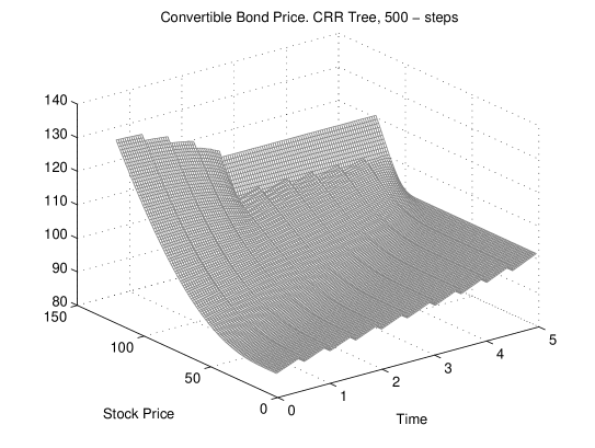
Figure 1: CB price, 500 steps

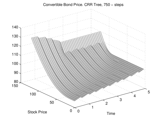
Figure 2: CB price, 750 steps

Figure 3: CB price profile at $t=2$

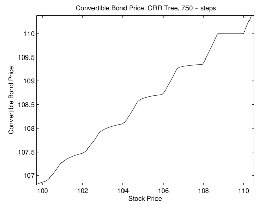
Figure 4: CB price profile at $t=2$

3.2 CB Delta and Gamma Sensitivities

Convertible bond delta and gamma quantify the sensitivity of the convertible price with respect to a small change in the underlying stock.
CB delta sometimes referred to as hedge ratio, is the number of units of the stock we should short for each CB that we hold in order to create a risk-less portfolio. On the other hand, it is the slope of the curve that relates the CB price to the underlying stock price. Thus, the natural definition of CB delta is

$$\Delta=\frac{\partial V}{\partial{S}}.$$

Traders and market makers prefer to use the following form of delta to illustrate the equity sensitivity of the convertible bond ([9], p. $23$)

$$\Delta_{\%}=\frac{\Delta}{C_{r}}$$

where $C_{r}$ refers to the conversion ratio (the number of shares per 100 nominal that bond holder gets when converting the bond). This number ranges between 0 and 100% whereas the previous delta definition would have values in the interval $[0,C_{r}]$.
CB gamma is a representative measure for convexity or non-linearity of the instrument. It measures the change in $\Delta$ for a change in the price of the underlying common stock.

$$\Gamma=\frac{\partial^{2}V}{\partial^{2}S}=\frac{\partial\Delta}{\partial S}$$

From a hedging point of view, CB gamma illustrates how often the position must be re-hedged in order to maintain a delta-neutral position. That is, if gamma is small, delta changes slowly, and adjustments to keep a position delta-neutral need to be made only relatively infrequently. However, if the absolute value of gamma is large, delta is highly sensitive to the price of the underlying asset. It is then quite risky to leave a delta-neutral position unchanged for any length of time.
As we have seen, the path dependency and the possibilities of terminating the bond before the maturity date, prohibit the derivation of a closed form pricing formula. Thus, the absence of closed form formula imposes the use of numerical methods to calculate the Greeks.
Finally, let us remark that it is a notorious fact that finite differences provide a bad approximation to delta and gamma, and are also computationally expensive. A satisfactory approach has been given for the computation of delta in ([2], [3]) and for the computation of gamma, in ([3]), and we will follow these references.
Within the Binomial-tree framework convertible bond delta is defined by (cf. [2], p. $398,$ formula (1.8), p. $170$ ):

$$\Delta=\Delta\left(t,S\right)=\frac{V^{+}-V^{-}}{(u-d)S},$$

where $t$ is the time and $S$ is the stock price at time zero; $u$ and $d$ are the parameters of the CRR tree, and $V_{1,1}$ and $V_{1,0}$ are estimated convertible bond values at one step forward when the stock price is $uS$ and $dS$ respectively.
In a similar way, the convertible bond gamma is defined by

$$\Gamma=\Gamma\left(t,S\right)=\frac{\Delta^{+}-\Delta^{-}}{(u-d)S},$$

where $\Delta^{+}$ is the value of delta at one step forward for the stock price $Su$, and $\Delta^{-}$ is the value of delta at one step forward for the stock price $Sd$.
Now, let us come back to market activities as pricing (Dollar Nuking or Delta Neutral pricing, [9]), analyzing and hedging where the existence of delta is of crucial importance.
Using the example from Table 1, in this section we demonstrate that throughout half of the CB life-span there exist stock prices for which the convertible bond delta is not well defined and atypically oscillates although the computation that we have made where based on large number of time steps. Similarly to the results of delta, the results for the convertible bond gamma are quite inconsistent.
In support of the above statements, in Figure 5 and Figure 6 we present the evolution of the CB delta and gamma during the time till maturity using a binary tree with 500 time steps. As before, the time value 0 corresponds to the issue date, and the time value 5, corresponds to the maturity date. Also, in order to ease the reader, we look at 2 years after the issue date, and in Figure 7 and Figure 8 we exhibit the profile of CB delta and gamma on the basis of 500 tree steps, namely the one-dimensional sections $\Delta\left(2,S\right)$ and $\Gamma\left(2,S\right).$ Both figures in identical way highlight the wrong performance of the approach corresponding to convertible bond delta and gamma.

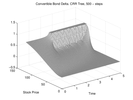
Figure 5: CB delta, 500 steps

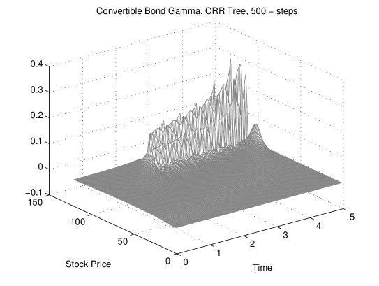
Figure 6: CB gamma, 500 steps

Figure 7: CB delta profile at $t=2$

Figure 8: CB gamma profile at $t=2$

3.3 Delta-Hedging (Convertible Arbitrage) of CB

The Delta-hedging in the case of CBs is called Convertible arbitrage.

Convertible arbitrage is a market-neutral investment strategy often employed by hedge funds (arbitrageurs). It involves the simultaneous purchase of convertible securities and the short sale of the same issuer’s common stock.

The number of shares sold short usually reflects a delta-neutral or market-neutral ratio. As a result, under normal market conditions, the arbitrageur expects the combined position to be insensitive to fluctuations in the price of the underlying stock.

A main reason for the popularity of Binary tree methods is that in the financial math community the following myths are widely spread: first, the delta-hedging is only possible in Binary tree framework and Black-Scholes framework, and second, the Binomial delta becomes, in the limit of time, the BS delta.

In real life situations the arbitrageurs expect that the Hedged position is insensitive with respect to the fluctuations in the price of the underlying stock.

In the following example we provide the graph of the relative change of the convertible arbitrage strategy (hedged position) calculated by means of the Binomial-tree, where the shock of the stock price is equal to $0.5$. The contract size of the position of CB given by Table 1 is $1.000.000,$ which is a realistic example. We assume that the settlement date is the issue date $t.$ The Delta-Hedged position (representing the convertible arbitrage strategy) is given by

$$\Pi\left(S\right)=V\left(S,t\right)-\frac{\partial V\left(S,t\right)}{\partial S}\cdot S$$

while its variation (resulting by the $0.5$ shock) is given by

$$\Pi\left(S+0.5\right)=V\left(S+0.5,t\right)-\frac{\partial V\left(S,t\right)}{\partial S}\cdot\left(S+0.5\right).$$

The increment (the change) $\Pi\left(S\right)$ of the portfolio is given by the difference

$$\Pi\left(S+0.5\right)-\Pi\left(S\right)=V\left(S+0.5,t\right)-V\left(S,t\right)-0.5\cdot\frac{\partial V\left(S,t\right)}{\partial S}.$$

On Figure 9 below we see that the Binomial-tree with $500$ steps does not meet the expectations of the arbitrageur since it oscillates considerably.

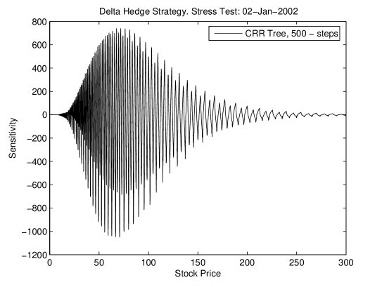
Figure 9: Delta Hedge strategy Stress Test

3.4 Risk Assessment

As an example of the bad performance of the Binomial-tree approximation to Risk Assessment we will present a simple case of Market Risk Assessment.
Market risk assessment explores the impact of market observable variables over the value of an investment (single position or a portfolio). Such variables are stock prices, interest rates, exchange rates etc. which are sometimes referred to as market risk drivers or simply risk drivers.
A commonly used methodology for estimation of market risk is Value-at-Risk (VaR), (see e.g. [6]). The importance of VaR arises from the fact that regulators and the financial industry advisory committees recommend VaR as way of measuring risk. The real boost in the use of VaR came when the Basel Committee on Banking Supervision adopted banks to use VaR as an internal model to set their capital requirements.
The $\operatorname*{VaR}$ measure is the highest possible loss over a certain period of time $h$ at a given confidence level ([6], [9]). The $\operatorname*{VaR}$ with confidence level $1-\alpha$ is defined as

$$\operatorname*{VaR}\nolimits_{1-\alpha}=-\min\left\{x{:P(X<=x)>\alpha}\right\}.$$

Here $1-\alpha$ is the confidence level, $\alpha$ usually takes values like $1\%$ or $5\%$ and $X$ is the change in the portfolio value, i.e. $X=V_{h}-V_{0}$. As usually portfolio values $V_{0}$ and $V_{h}$ correspond to the initial time and the end of the holding period. The mostly used holding period, over which the expected convertible bond loss is calculated, is one day or one month (22 business days).
It is clear that to calculate $\operatorname*{VaR}$ values we need the probability density function of the portfolio value. The $\operatorname*{VaR}$ methodologies mainly differ in ways of constructing the probability density function. The widely used in practice are the following methodologies ([6], [9]):

• Parametric method;

• Historical simulation;

• Monte Carlo simulation.

We will apply the mostly used third method, namely, the MC simulation. The reason is that the Parametric method is based on delta and gamma valuation and we have seen in the previous section that their computation by means of the Binomial-tree is inefficient. Also, the application of the Historical method would require to tie down the evidence with a partial historical environment.

Let us point out, that the use of Binomial-tree approach in building a $\operatorname*{VaR}$ methodology is too inadequate, due to the fact that the probability density function in many examples of CBs is inadequate. In support of this statement we consider the typical CB example considered in Table 1 and provide its simplified $\operatorname*{VaR}$ analysis as described in Table 2.

Table 2: VaR analysis conditions

Parameter	Value
Pricing Model	CRR tree with 500 time steps
Evaluation Date	2-Jan-2004
Holding Period	1 day
Confidence level	99%
Source of risk	Underlying Stock, only
Stock Price Scenario type	Log-normal: mean = 0.05, variance = 30%
Number of Scenarios	10000
Stock Spot Price	100

Although the $\operatorname*{VaR}$ value at $99\%$ given by $\operatorname*{VaR}_{99}=1.1285\%$ looks good as a level of risk, in fact it and all other $\operatorname*{VaR}$ values are very questionable since they are obtained from the wrongly constructed probability density $\rho.$ Indeed, we compute the density $\rho$ by means of MC simulation for the underlying stock that are valid for the end of the holding period. In Figure 10 we see that $\rho$ exhibits the atypical movements of probability mass caused by the atypical price profile of CB price at the end of the holding period. Finally, for completeness sake, in Figure 11 we show Monte Carlo scenarios for the underlying stock which are valid for the end of the holding date.

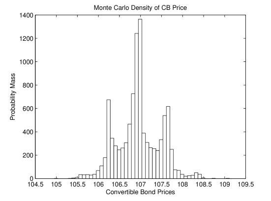
Figure 10: MC density of CB price

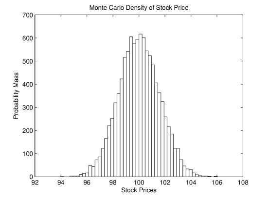
Figure 11: MC density of stock price

4 Conclusion

In this paper we have made performance evaluation of the widely used and popular techniques of Binomial-tree for approximation of the Tsiveriotis-Fernandes model for price dynamics of CBs. Our results show that in many typical examples the Binomial-tree techniques do not meet practitioners’ criteria. Let us mention that even the simplest FDS technique (the explicit method) has much better performance and this will be the subject of our next paper.

5 Appendix. The model of Tsiveriotis-Fernandes (TF)

For reader’s convenience in the present section we provide the Tsiveriotis-Fernandes (TF) model for computation of the Convertible Bonds.

The pricing of CB has two main periods: before $1998$, and after $1998$ when the Tsiveriotis-Fernandes model has appeared, [1]. It represents a major breakthrough in the area which revolutionized the price computation.

First of all, the system of TF represents a prettily complicated system of equations which has solutions with free boundary. This makes it much more complicated for analysis and numerical solution than the American options. For that reason a Binomial-tree model represents a very intuitive approximation to the model of TF, and this is completely analogous to the situation in Options theory where Binomial-tree models are very popular.

The idea of the TF model is that the CB price $V$ is represented as a sum of two components

$$V=B+E$$

where $B$ is the Cash Component, and $E$ is the Equity Component.

$B$ is related to the future payments in cash, given at moment $t$. Then we can construct a risk neutral portfolio

$$\Pi=B-\Delta S.$$

In case of no default in the time interval $[t,t+\delta t]$, for

$$d\Pi=\Pi_{t+\delta t}-\Pi_{t}$$

we have

$$d\Pi=(B_{t}+\frac{1}{2}\sigma^{2}S^{2}B_{S}S)dt.$$

On the other hand, on default in the same time interval the model assumption is that the bond holder will lose all future cash flows, that is

$$d\Pi=-B.$$

Because of this, the expected value of $d\Pi$ is equal to

$$E(d\Pi)=(B_{t}+\frac{1}{2}\sigma^{2}S^{2}B_{S}S-r_{c}B)dt$$

Finally, from non-arbitrage arguments

$$B_{t}+\frac{1}{2}\sigma^{2}S^{2}B_{SS}+rSB_{S}-(r+r_{c})B=0.$$

On the other hand the value $E=V-B$ represents the value of the CB related to payments in equity, and it should therefore satisfy the Black-Scholes equation

$$(V-B)_{t}+\frac{1}{2}\sigma^{2}S^{2}(V-B)_{SS}+rS(V-B)_{S}-r(V-B)=0.$$

Now, replacing the equation for $B$ we obtain equation

$$V_{t}+\frac{1}{2}\sigma^{2}S^{2}V_{SS}+rSV_{S}-rV-r_{c}B=0.$$

Thus we have the system of two equations:

$$\begin{split}&V_{t}+\frac{1}{2}\sigma^{2}S^{2}V_{SS}+rSV_{S}-rV-Br_{c}=0\\ &B_{t}+\frac{1}{2}\sigma^{2}S^{2}B_{SS}+rSB_{S}-(r+r_{c})B=0\end{split}$$

where:

$\qquad V$ - price of CB

$\qquad B$ - price of cash-only part of the CB

$\qquad S$ - stock price, $S\in[0,\infty)$

$\qquad k$ - conversion ratio

$\qquad N$ - nominal (par value) of the CB

$r$ - risk-free rate

$\qquad r_{c}$ - the yield spread, or credit spread

$\qquad t$ - evaluation date, $t\in[0,T]$

$\qquad T$ - maturity date

We have the ”conversion function”:

$$cnv\left(S,t\right):=\left\{\begin{array}[c]{l}k\cdot S\qquad\text{if }t\in\text{{Conversion periods} of the Contract}\\ 0\qquad\text{otherwise}\end{array}\right.$$

The ”Put Back function” is defined by

$$B^{Put}\left(t\right)=\left\{\begin{array}[c]{l}b\left(t\right)\qquad\text{for }t\in\text{ {Put periods} of the Contract}\\ 0\qquad\text{otherwise}\end{array}\right.$$

for a Contracted function $b\left(t\right);$

The ”Call Back function” is defined by

$$B^{Call}(t)=\left\{\begin{array}[c]{l}c\left(t\right)\qquad\text{for }t\in\text{ {Call periods} of the Contract}\\ +\infty\qquad\text{otherwise}\end{array}\right.$$

We have the following Boundary Conditions and Constraints:

$$\begin{array}[c]{l}\mathbf{Expiry}\text{ }\mathbf{Conditions\quad}\text{for }t=T\\ \quad V(S,T)=\max(cnv(S,T),N)\\ \quad B(S,T)=\left\{\begin{array}[c]{ll}N,&cnv(S,T)\leq N\\ 0,&\text{otherwise}\end{array}\right.\end{array}$$

and the

$$\begin{array}[c]{l}\mathbf{Boundary}\text{ }\mathbf{Conditions\quad}\text{for }S=0\text{ and }S=\infty\\ \quad\begin{array}[c]{l}\text{when }S=0,\ 0\leq t\leq T\\ \qquad V(0,t)=\max(B^{Put}(t),V(t))\\ \qquad B(0,t)=\max(B^{Put}(t),B(t))\\ \\ \quad\quad\text{where }V=V(t)\text{ and }B=B(t)\text{ are}\\ \qquad V(t)=B(t)=N\cdot e^{-(r+r_{c})(T-t)}\\ \\ \text{when }S\longrightarrow\infty:\ \text{for }0\leq t\leq T\\ \qquad V(S,t)=cnv(S,T),\ \ B(S,t)=0\end{array}\end{array}$$

The Payoff Constraints: 

$$\begin{array}[c]{l}V(S,t)=\max(B^{Put}(t),cnv(S,t),\min(B^{Call}(t),V_{held}(S,t)))\\ 0\leq S<+\infty,\ 0\leq t<T\end{array}$$

We have to note that all conditions and constraints above are for zero coupon CB which is enough for our present considerations.

E-mail adresses: K. Milanov, kpacu.milanov@gmail.com ; O. Kounchev, kounchev@gmx.de

References

- [1] Tsiveriotis, K. and Fernandes, C. (1998, September) ‘Valuing Convertible Bonds with Credit Risk’, Journal of Fixed Income, Vol. 8, pp. 95–102.
- [2] Hull, J. Options, Futures and Other Derivatives, 5th edition. Prentice-Hall, Upper Saddle River NJ, 2002.
- [3] Wilmott, P. DERIVARIVES: The Theory and Practice of Financial Engineering. John Wiley & Sons, 2000.
- [4] Andersen, L. and Buffrum, D. (2002, October) ‘Calibration and Implementation of Convertible Bond Models’, Working Paper, Bank of America Securities.
- [5] Ayache, E., P.A. Forsyth, and Vetzal, K., ‘Valuation of Convertible Bonds With Credit Risk’, The Journal of Derivatives Vol. 11, pp. 9-29, Fall 2003.
- [6] Fabozzi, F. and Rachev, Z., Fat-Tailed and Skewed Asset Return Distributions. Implications for Risk Management, portfolio Selection, and Option Pricing. John Wiley & Sons, 2005.
- [7] Gushchin, V. and Curien, E. (2008, July), ‘The pricing of Convertible Bonds within Tsiveriotis and Fernandes framework with exogenous credit spread: Empirical Analysis’, Journal of Derivatives & Hedge Funds Vol. 14, pp. 50–64.
- [8] Zabolotnyuk, Y., Jones, R. and Veld, C., ‘An EmpiricalL Comparison of Convertible Bond Valuation Models’, Financial Management Volume 39, Issue 2, pages 675–706, Summer 2010.
- [9] De Spiegeleer, J. and Schoutens, W., The Handbook of Convertible Bonds: Pricing, Strategies and Risk Management. The Wiley Finance Series, 2011.
- [10] Citigroup, ‘Convertible Bonds. A Guide’ (2003, December)