Hawking temperature for near-equilibrium black holes

Abstract

We discuss the Hawking temperature of near-equilibrium black holes using a semiclassical analysis. We introduce a useful expansion method for slowly evolving spacetime, and evaluate the Bogoliubov coefficients using the saddle point approximation. For a spacetime whose evolution is sufficiently slow, such as a black hole with slowly changing mass, we find that the temperature is determined by the surface gravity of the past horizon. As an example of applications of these results, we study the Hawking temperature of black holes with null shell accretion in asymptotically flat space and the AdS–Vaidya spacetime. We discuss implications of our results in the context of the AdS/CFT correspondence.

I Introduction

The fact that black holes possess thermodynamic properties has been intriguing in gravitational and quantum theories, and is still attracting interest. Nowadays it is well-known that black holes will emit thermal radiation with Hawking temperature proportional to the surface gravity of the event horizon Hawking:1974sw . This result plays a significant role in black hole thermodynamics. Moreover, the AdS/CFT correspondence Maldacena:1997re opened up new insights about thermodynamic properties of black holes. In this context we expect that thermodynamic properties of conformal field theory (CFT) matter on the boundary would respect those of black holes in the bulk. In particular, stationary black holes correspond to thermal equilibrium of the dual field theory at finite temperature equal to the bulk Hawking temperature Witten:1998zw .

It is interesting to study if such thermal properties persist when time dependence is turned on. From a technical viewpoint, the original derivation of the Hawking radiation Hawking:1974sw was performed on a static or stationary background (precisely speaking, as an approximation at late time), and it is not obvious how to accommodate dynamical spacetimes into the scheme. From a physical viewpoint, such a study can be useful since realistic black holes in our universe are dynamical or at least quasistationary. For example, processes like black hole formation after a gravitational collapse or black hole evaporation due to the Hawking radiation may involve highly time-dependent phases, and it is not obvious how the Hawking radiation will behave in such systems.

When time dependence is sufficiently weak, however, we may expect thermodynamic properties of a black hole to persist. This expectation partially stems from physical insight on ordinary thermodynamics systems, in which thermodynamic properties persists when the system is sufficiently near equilibrium and quasistationary. If black hole thermodynamics is robust enough, such insight on usual thermodynamic systems leads to the above expectation on dynamical spacetimes and black holes. Many studies have been made on generalizing Hawking temperature for dynamical black hole approaches Harada:2000ar ; Saida:2007ru ; Nielsen:2007ac ; Hayward:2008jq ; Barcelo:2010pj ; Barcelo:2010xk ; Mazumder:2011gk , and they support such an expectation.

Within the context of the AdS/CFT correspondence, thermodynamic properties of dynamical black holes lead to new insights into the dynamics of strongly coupled field theory on the boundary. One typical problem in this line is thermalization processes in the boundary field theory, which is holographically modeled by formation of the bulk black hole and its equilibration into a stationary state. Much effort is devoted to such problems in connection with, for example, application of the AdS/CFT correspondence to QCD physics like that in the RHIC experiment, or to nonequilibrium phenomena in condensed matter physics and fluid dynamics Son:2002sd ; Janik:2006gp ; Kinoshita:2008dq ; Chesler:2008hg ; Murata:2010dx ; Das:2010yw ; Hubeny:2010ry ; Ebrahim:2010ra ; Hashimoto:2010wv ; Erdmenger:2011jb ; CaronHuot:2011dr ; Balasubramanian:2011ur ; Garfinkle:2011hm . In this context, the Hawking radiation in the bulk is interpreted as quantum fluctuation in the boundary theory, and it plays an important role in certain setups deBoer:2008gu ; Aharony:2005bm .

Based on these interests, in this paper we consider nonstationary spacetimes, and try to determine the Hawking temperature measured by observers in the asymptotic region. One naive way to do this would be to define a certain time coordinate to associate temperature of the black hole (future) horizon to that measured by asymptotic observers. Even though this procedure is seemingly natural from the viewpoint of black hole thermodynamics or horizon dynamics, it is puzzling from the viewpoint of causality, since this temperature is determined using information in the future region for that observer. In the AdS/CFT setup, if we were to define temperature at a point on the boundary in this way, we would need information in the bulk region, which is not causally accessible from that boundary point. Such a property would not be desirable if we care about causality in the bulk and boundary, especially when time dependence comes into the story.

To avoid such problems, we consider the conventional derivation of the Hawking radiation based on Bogoliubov transformations for nonstationary background. An advantage of this method is that we can naturally determine temperature measured by asymptotic observers using only information causally available to them. Particularly, we focus our attention on an eternal black hole rather than black hole formation by gravitational collapse because we are interested in near-equilibrium system such as transition from an equilibrium state to another equilibrium state. In other words, we focus on late-time dynamics after the black hole has formed. We clarify how the Hawking temperature changes when a black hole becomes dynamical, for instance, due to mass accretion to the black hole, and show that the Hawking temperature of dynamical black holes can be naturally associated with “surface gravity” of the past horizon.

The paper is organized as follows. In Sec. II, we evaluate the Bogoliubov coefficients using the saddle point approximation and show that the “surface gravity” of the past horizon gives the Hawking temperature observed in the asymptotic region. In Sec. III, as illustrations of the use of our method, we consider applications to simple examples in asymptotically flat and AdS cases. We summarize and discuss implications of the results in Sec. IV.

II Estimation of Bogoliubov coefficients

We estimate Bogoliubov coefficients in order to define Hawking temperature for a nonstationary background in this section. We consider an eternal black hole in thermal equilibrium with its surroundings, that is, in the Hartle–Hawking state. In asymptotically flat cases, we should immerse the black hole into a thermal bath to realize this state. In asymptotically AdS cases, on the other hand, it is naturally realized due to its boundary condition Klemm:1998bb ; Hemming:2000as because the black hole is enclosed in the AdS boundary.

We exploit the saddle point approximation to evaluate the Bogoliubov coefficients and determine the temperature from them. After reviewing usage of the approximation for the static spacetime in Sec. II.1, we consider its extension to nonstationary spacetime in Sec. II.2. In this extension to nonstationary spacetime, we introduce a quantity, $\kappa(u)$, which may be interpreted as an extension of the surface gravity of static Killing horizon. In Sec. II.3, we reinterpret this quantity from a geometric point of view, and clarify that $\kappa(u)$ is naturally associated with the past horizon of the eternal black hole.

II.1 Static spacetime and the saddle point approximation

For simplicity, we consider the two-dimensional part of the spacetime consisting of time and radial directions, that is, we focus on the s-wave sector of radiation. We also adopt the geometric optics approximation, and neglect the backscattering of the waves due to the curvature of spacetime. We introduce the null coordinate $u$ which gives a natural time for observers in the asymptotic region (null infinity). If the spacetime is stationary, this time corresponds to the Killing time. We introduce another null coordinate $U$ which is the affine parameter on the past horizon. For the stationary case it becomes the familiar Kruskal coordinate. Because lines described by $u=\text{const.}$ are outgoing null geodesics, geodesic equations give a relation $U=U(u)$ between the two null coordinates.

Now, we consider a massless scalar field. In the current setup, solutions of the field equation are simply given by arbitrary functions of each null coordinate. In a standard manner we can define positive frequency modes with respect to $u$ and $U$, respectively. Then, the Bogoliubov transformation between two sets of modes $u_{\omega}\propto e^{-i\omega u}$ and $\bar{u}_{\hat{\omega}}\propto e^{-i\hat{\omega}U}$ is determined by the Bogoliubov coefficients

$$\left.\begin{aligned} \alpha_{\omega\hat{\omega}}\\ \beta_{\omega\hat{\omega}}\end{aligned}\right\}=\pm\frac{i}{2\pi}\sqrt{\frac{\hat{\omega}}{\omega}}\int^{\infty}_{-\infty}\mathrm{d}u\frac{\mathrm{d}U}{\mathrm{d}u}e^{\pm i\omega u-i\hat{\omega}U(u)},$$ (1)

where the upper and lower signs correspond to $\alpha_{\omega\hat{\omega}}$ and $\beta_{\omega\hat{\omega}}$, respectively.

Now, to evaluate those coefficients by the saddle point approximation, we will consider the integral

$$\int^{\infty}_{-\infty}\exp\phi(u)\mathrm{d}u,$$ (2)

where

$$\phi(u)\equiv\log\frac{\mathrm{d}U}{\mathrm{d}u}\pm i\omega u-i\hat{\omega}U(u).$$ (3)

Saddle points are located at $u=u_{*}$ given by $\phi^{\prime}(u_{*})=0$, where

$$\phi^{\prime}(u)=\frac{\mathrm{d}}{\mathrm{d}u}\log\frac{\mathrm{d}U}{\mathrm{d}u}\pm i\omega-i\hat{\omega}\frac{\mathrm{d}U}{\mathrm{d}u},$$ (4)

and a prime denotes a derivative.

Consider a static black hole, for example. When the surface gravity at the Killing horizon is $\kappa$, the relation between the two coordinates $u$ and $U$ is given by $U(u)=-\exp(-\kappa u)$, which is the coordinate transformation for the Kruskal coordinate. Then, we have

$$\phi^{\prime}(u_{*})=-\kappa\pm i\omega-i\hat{\omega}\kappa e^{-\kappa u_{*}}=0,$$ (5)

and the saddle point

$$u_{*}=-\kappa^{-1}\log\left(\frac{ire^{\mp i\theta}}{\hat{\omega}}\right)=-\frac{1}{\kappa}\log\frac{r}{\hat{\omega}}-\frac{i}{\kappa}\left(\frac{\pi}{2}\mp\theta\right),$$ (6)

where $re^{\mp i\theta}\equiv 1\mp i\omega/\kappa$. We notice that the real part of $u_{*}$ depends on $\hat{\omega}$ and it becomes larger as $\hat{\omega}$ increases. This implies that the Kruskal modes with very high frequencies $\hat{\omega}$ are relevant for late-time features, while relevant frequencies $\hat{\omega}$ will change depending on the time of observation. [See also discussions around Eq. (30).] Using

$$\phi(u_{*}) =\log\kappa+re^{\mp i\theta}\log\left(\frac{ire^{-1\mp i\theta}}{\hat{\omega}}\right),$$ (7)

$$\phi^{\prime\prime}(u_{*}) =-\kappa^{2}re^{\mp i\theta},$$

we have the saddle point approximation of the integral (2) as

$$\int^{\infty}_{-\infty}e^{\phi(u)}\mathrm{d}u\simeq e^{\phi(u_{*})}\int^{\infty}_{-\infty}e^{\frac{\phi^{\prime\prime}(u_{*})}{2}(u-u_{*})^{2}}\mathrm{d}u=e^{\phi(u_{*})}\sqrt{\frac{2\pi}{-\phi^{\prime\prime}(u_{*})}}=\kappa\left(\frac{ire^{-1\mp i\theta}}{\hat{\omega}}\right)^{re^{\mp\theta}}\sqrt{\frac{2\pi}{re^{\mp i\theta}}},$$ (8)

which becomes a good approximation when $\omega/\kappa\gg 1$. This expression derives the Bogoliubov coefficients of Eq. (1) given by

$$\frac{|\alpha_{\omega\hat{\omega}}|^{2}}{|\beta_{\omega\hat{\omega}}|^{2}}\simeq\exp\left(\frac{2\pi\omega}{\kappa}\right).$$ (9)

Thus, we have the familiar result of the Hawking temperature to be $T=\kappa/2\pi$ by the saddle point approximation.

We could also perform the integral explicitly to obtain a well-known exact expression Hawking:1974sw

$$\int^{\infty}_{-\infty}e^{\phi(u)}\mathrm{d}u=\kappa(-i\hat{\omega})^{-re^{\mp i\theta}}\Gamma\left(re^{\mp i\theta}\right).$$ (10)

Using the Stirling formula of the gamma function

$$\Gamma(1+z)=z\Gamma(z)\simeq\sqrt{2\pi z}\left(\frac{z}{e}\right)^{z},$$ (11)

we have Eq. (8) again from Eq. (10). This result indicates that when the geometric optics approximation is satisfied, namely, when $\omega/\kappa\gg 1$, the saddle point approximation is valid.

II.2 Extension to nonstationary spacetime

Let us now take a nonstationary spacetime background. To probe this spacetime, we use wave packets which are localized in both the time and frequency domains rather than plane waves spreading over the whole time. The wave packet is peaked around a time $u=u_{0}$ with width $\sim\Delta u$, which are the time and duration of the observation, respectively. The Bogoliubov coefficients for a wave packet are obtained by inserting a window function into the integrand of Eq. (1), that is,

$$\left.\begin{aligned} A_{\omega\hat{\omega}}\\ B_{\omega\hat{\omega}}\end{aligned}\right\}=\pm\frac{1}{2\pi}\sqrt{\frac{\hat{\omega}}{\omega}}\int^{\infty}_{-\infty}w_{\Delta u}(u-u_{0})\frac{\mathrm{d}U}{\mathrm{d}u}e^{\pm i\omega u-i\hat{\omega}U(u)}\mathrm{d}u,$$ (12)

where $w_{\Delta u}(x)$ is a window function which goes sufficiently fast to zero outside the interval $\Delta u$ around $x=0$. In addition, we assume that analytic continuation of $w_{\Delta u}(x)$ is varying slowly at least for $|x|<\Delta u$ in the complex plane. Using the Klein–Gordon product, these coefficients are written as $A_{\omega\hat{\omega}}=(\psi_{\omega},\bar{u}_{\hat{\omega}})$ and $B_{\omega\hat{\omega}}=-(\psi^{*}_{\omega},\bar{u}_{\hat{\omega}})$, where we have constructed the wave packet localized around time $u=u_{0}$ and frequency $\omega$ as

$$\psi_{\omega}(u)=\frac{1}{\sqrt{4\pi\omega}}w_{\Delta u}(u-u_{0})e^{-i\omega u}.$$ (13)

We note that $A_{\omega\hat{\omega}}$ and $B_{\omega\hat{\omega}}$ satisfy the following relation

$$\int^{\infty}_{0}\mathrm{d}\hat{\omega}\left(|A_{\omega\hat{\omega}}|^{2}-|B_{\omega\hat{\omega}}|^{2}\right)=(\psi_{\omega},\psi_{\omega}),$$ (14)

which follows from the completeness of $\{\bar{u}_{\hat{\omega}}\}$. The number density in terms of the wave packet mode $\psi_{\omega}$ is given by

$$\frac{1}{(\psi_{\omega},\psi_{\omega})}\int^{\infty}_{0}\mathrm{d}\hat{\omega}|B_{\omega\hat{\omega}}|^{2},$$ (15)

which is roughly the number of particles generated in the frequency band of width $\sim 1/\Delta u$ around frequency $\omega$.

Let us suppose that the evolution of the background spacetime is sufficiently slow around $u=u_{0}$ within time interval $\Delta u$. To clarify what slowly evolving is, we shall introduce the following quantity

$$\kappa(u)\equiv-\frac{\mathrm{d}}{\mathrm{d}u}\log\frac{\mathrm{d}U}{\mathrm{d}u}.$$ (16)

If the background spacetime is stationary, $\kappa(u)$ becomes a constant and it is nothing but the surface gravity of the black hole (Killing) horizon, as we have seen in the previous section. Therefore, we may state that the spacetime is evolving slowly when $\kappa(u)$ is almost constant during $\Delta u$. In that case, we may express $\kappa(u)$ as

$$\kappa(u)=\kappa_{0}\left[1+\epsilon f(u)\right],$$ (17)

where $f(u)$ is a real function which satisfies $f(u_{0})=0$ and $|f(u)|\leq 1$ for $|u-u_{0}|<\Delta u$, and $\epsilon$ is a small parameter. In other words, this assumption implies

$$\frac{\Delta\kappa}{\kappa_{0}}\leq\epsilon\quad\text{for}\quad|u-u_{0}|<\Delta u,$$ (18)

where $\Delta\kappa\equiv|\kappa(u)-\kappa_{0}|$. For discussions below, we further assume that analytic continuation of $f(u)$ satisfies $|f(u)|\leq 1$ for any complex $u$ such that $|u-u_{0}|<\Delta u$.

Then, we may expand $U^{\prime}(u)$, $U(u)$ and $U^{\prime\prime}(u)$ with respect to $\epsilon$ as

$$U^{\prime}(u) =U^{\prime}_{0}\exp\left(-\int_{u_{0}}^{u}\kappa(x)\mathrm{d}x\right)=U^{\prime}_{0}\exp\left\{-\kappa_{0}\left(\delta u+\epsilon g(u)\right)\right\}=U^{\prime}_{0}e^{-\kappa_{0}\delta u}\left(1-\epsilon\kappa_{0}g(u)+\mathcal{O}(\epsilon^{2})\right),$$ (19)

$$U(u) =U_{0}+\int_{u_{0}}^{u}U^{\prime}(x)\mathrm{d}x=U_{0}+U^{\prime}_{0}\left(\frac{1-e^{-\kappa_{0}\delta u}}{\kappa_{0}}-\epsilon\kappa_{0}\int_{u_{0}}^{u}e^{-\kappa_{0}(x-u_{0})}g(x)\mathrm{d}x+\mathcal{O}(\epsilon^{2})\right),$$

$$U^{\prime\prime}(u) =-\kappa(u)U^{\prime}(u)=-\kappa_{0}\left(1+\epsilon f(u)\right)U^{\prime}_{0}e^{-\kappa_{0}\delta u}\left(1-\epsilon\kappa_{0}g(u)+\mathcal{O}(\epsilon^{2})\right),$$

where we defined $U_{0}=U(u_{0})$, $\delta u=u-u_{0}$ and

$$g(u)=\int_{u_{0}}^{u}f(x)\mathrm{d}x.$$ (20)

Note that $|g(u)|\leq|\delta u|$ follows from the assumption $|f(u)|\leq 1$ for $|\delta u|<\Delta u$. We also expand the saddle point $u=u_{*}$ as

$$u_{*}=u_{*}^{(0)}+\epsilon u_{*}^{(1)}+\mathcal{O}(\epsilon^{2}).$$ (21)

Then, the equation for the saddle point from Eq. (4) is expanded using Eq. (19) as

$$0=\phi^{\prime}(u_{*})=-\kappa_{0}re^{\mp i\theta}-i\hat{\omega}U^{\prime}_{0}e^{-\kappa_{0}\delta u_{*}^{(0)}}+\epsilon\kappa_{0}\left[-f\bigl{(}u_{*}^{(0)}\bigr{)}+i\hat{\omega}U^{\prime}_{0}e^{-\kappa_{0}\delta u_{*}^{(0)}}\left(u_{*}^{(1)}+g\bigl{(}u_{*}^{(0)}\bigr{)}\right)\right]+\mathcal{O}(\epsilon^{2}),$$ (22)

where we have redefined $re^{\mp i\theta}\equiv 1\mp i\omega/\kappa_{0}$, which satisfies $r\gg 1$ because of the geometric optics approximation $\omega/\kappa_{0}\gg 1$. Solving $\phi^{\prime}(u_{*})=0$ order by order of $\epsilon$, we find

$$\delta u_{*}^{(0)}= -\kappa_{0}^{-1}\log\left(\frac{i\kappa_{0}re^{\mp i\theta}}{\hat{\omega}U^{\prime}_{0}}\right)=-\frac{1}{\kappa_{0}}\log\left(\frac{\kappa_{0}r}{\hat{\omega}U^{\prime}_{0}}\right)-\frac{i}{\kappa_{0}}\left(\frac{\pi}{2}\mp\theta\right),$$ (23)

$$u_{*}^{(1)}= -g\bigl{(}u_{*}^{(0)}\bigr{)}+\frac{e^{\kappa_{0}\delta u_{*}^{(0)}}}{i\hat{\omega}U^{\prime}_{0}}f\bigl{(}u_{*}^{(0)}\bigr{)}=-g\bigl{(}u_{*}^{(0)}\bigr{)}-\frac{f\bigl{(}u_{*}^{(0)}\bigr{)}}{\kappa_{0}re^{\mp i\theta}}~{}.$$

Plugging Eq. (23) into Eq. (3) and $\phi^{\prime\prime}(u)=-\kappa^{\prime}(u)-i\hat{\omega}U^{\prime\prime}(u)$ at $u=u_{*}$ and expanding with respect to $\epsilon$, we find $\phi(u_{*})-\phi(u_{0})\equiv\phi_{0}+\epsilon\phi_{1}$ and $\phi^{\prime\prime}(u_{*})\equiv\phi^{\prime\prime}_{0}+\epsilon\phi^{\prime\prime}_{1}$ are given by $\phi(u_{0})\equiv\log U^{\prime}_{0}\pm i\omega u_{0}-i\hat{\omega}U_{0}$,

$$\phi_{0}=-re^{\mp i\theta}\left(\kappa_{0}\delta u_{*}^{(0)}+1\right)-\frac{i\hat{\omega}U^{\prime}_{0}}{\kappa_{0}},\qquad\phi_{1}=-\kappa_{0}g\bigl{(}u_{*}^{(0)}\bigr{)}+i\hat{\omega}U^{\prime}_{0}\kappa_{0}\int_{u_{0}}^{u_{*}^{(0)}}e^{-\kappa_{0}\delta u}g(u)\mathrm{d}u$$ (24)

and

$$\phi^{\prime\prime}_{0}=-\kappa_{0}^{2}re^{\mp i\theta},\qquad\phi^{\prime\prime}_{1}=-\kappa_{0}\left(f^{\prime}\bigl{(}u_{*}^{(0)}\bigr{)}+\kappa_{0}\left(1+re^{\mp i\theta}\right)f\bigl{(}u_{*}^{(0)}\bigr{)}\right),$$ (25)

where $\mathcal{O}(\epsilon^{2})$ terms are omitted.

To guarantee that the perturbative expansion above is valid and that the calculation of the saddle point approximation is not affected by the correction terms, we should require each of correction terms [$\epsilon u_{*}^{(1)}$, $\epsilon\phi_{1}$ and $\epsilon\phi^{\prime\prime}_{1}$ in Eqs. (23), (24) and (25)] to be much smaller than their leading term ($\delta u_{*}^{(0)}$, $\phi_{0}$ and $\phi^{\prime\prime}_{0}$, respectively). As for $\epsilon\bigl{|}u_{*}^{(1)}\bigr{|}\ll\bigl{|}\delta u_{*}^{(0)}\bigr{|}$ and $\epsilon\bigl{|}\phi_{1}^{\prime\prime}\bigr{|}\ll\bigl{|}\phi_{0}^{\prime\prime}\bigr{|}$, we can see from Eqs. (23) and (25) that we should assume both $\epsilon\ll 1$ and $\bigl{|}f^{\prime}\bigl{(}u_{*}^{(0)}\bigr{)}\bigr{|}\ll\kappa_{0}r$ to hold to satisfy such requirements, where we used $|g(u)|\leq|\delta u|$. As for $\epsilon|\mathrm{Re}\,\phi_{1}|\ll|\mathrm{Re}\,\phi_{0}|$, we have

$$\mathrm{Re}\,\phi_{0}= \mp\omega\mathrm{Im}\,u^{(0)}_{*}-\kappa_{0}\mathrm{Re}\,\delta u^{(0)}_{*}-1,$$ (26)

$$\mathrm{Re}\,\phi_{1}= -\kappa_{0}\mathrm{Re}\,g\bigl{(}u^{(0)}_{*}\bigr{)}+\mathrm{Re}\left(i\hat{\omega}U^{\prime}_{0}\kappa_{0}\int^{\mathrm{Re}\,u^{(0)}_{*}+i\mathrm{Im}\,u^{(0)}_{*}}_{\mathrm{Re}\,u^{(0)}_{*}}e^{-\kappa_{0}\delta u}g(u)\mathrm{d}u\right),$$

and

$$|\mathrm{Re}\,\phi_{1}|<\kappa_{0}\bigl{|}\delta u^{(0)}_{*}\bigr{|}+\kappa_{0}^{2}r\bigl{|}\delta u^{(0)}_{*}\bigr{|}\bigl{|}\mathrm{Im}\,u^{(0)}_{*}\bigr{|}.$$ (27)

Then, for $\epsilon|\mathrm{Re}\,\phi_{1}|\ll|\mathrm{Re}\,\phi_{0}|$ to hold, we need to additionally require $\epsilon\kappa_{0}\bigl{|}\delta u^{(0)}_{*}\bigr{|}\ll 1$. Under these assumptions, we find that the integral in Eq. (12) can be evaluated by the saddle point approximation as

$$\left|\int^{\infty}_{-\infty}w_{\Delta u}(\delta u)e^{\phi(u)}\mathrm{d}u\right|\simeq U^{\prime}_{0}\left|w_{\Delta u}\bigl{(}\delta u_{*}^{(0)}\bigr{)}\right|e^{\mathrm{Re}\,\phi_{0}}\sqrt{\frac{2\pi}{|\phi^{\prime\prime}_{0}|}}~{}.$$ (28)

So that the suppression due to the window function, $w_{\Delta u}$, is weak and the integral value becomes close to that for the unwindowed function, the saddle point should satisfy $|\delta u_{*}|\lesssim\Delta u$. For the imaginary part of $u_{*}^{(0)}$ the condition $|\delta u_{*}|\lesssim\Delta u$ becomes

$$\frac{1}{\Delta u}\lesssim\kappa_{0},$$ (29)

and for the real part it becomes a condition on $\hat{\omega}$, given by

$$\frac{\kappa_{0}r}{U^{\prime}_{0}}e^{-\kappa_{0}\Delta u}\lesssim\hat{\omega}\lesssim\frac{\kappa_{0}r}{U^{\prime}_{0}}e^{\kappa_{0}\Delta u}.$$ (30)

If $\hat{\omega}$ is out of this region, no saddle point exists between $|u-u_{0}|\lesssim\Delta u$, and then the integral will be suppressed due to the window function. This condition means that only the Kruskal modes of $\hat{\omega}$ with limited frequency band, specified by Eq. (30), can have correlations with the wave packet mode $\psi_{\omega}$ due to its localization in the time domain.

Consequently, sufficient conditions for the saddle point approximation to be valid are given by

$$\epsilon\kappa_{0}\ll\frac{1}{\Delta u}\lesssim\kappa_{0}\ll\omega,\qquad\bigl{|}f^{\prime}(u)\bigr{|}\ll\kappa_{0}r,$$ (31)

for $|u-u_{0}|<\Delta u$. Note that the condition on $\epsilon$, $\epsilon\kappa_{0}\ll\Delta u^{-1}$, can be rewritten as $\Delta\kappa\Delta u\ll 1$, where $\Delta\kappa$ is defined by Eq. (18). If we can take the time interval $\Delta u(\gtrsim\kappa_{0}^{-1})$ satisfying this condition, we have a sufficiently small $\epsilon\ll 1$ for which Eq. (31) holds. Roughly speaking, this condition is indicating that the time variation of $\kappa(u)$ should be sufficiently moderate to satisfy $\frac{1}{\kappa_{0}^{2}}\frac{\mathrm{d}\kappa}{\mathrm{d}u}\ll 1$ between the interval $|u-u_{0}|\lesssim\kappa_{0}^{-1}$. Under these assumptions, at the leading order we have

$$\frac{|A_{\omega\hat{\omega}}|^{2}}{|B_{\omega\hat{\omega}}|^{2}}\simeq\exp\left(\frac{2\pi\omega}{\kappa_{0}}\right),$$ (32)

which implies the spectrum observed at the time $u=u_{0}$ becomes a thermal one with temperature $\kappa_{0}/2\pi$ for high frequencies $\omega\gg\kappa_{0}$.

II.3 Surface gravity for past horizon

In this section, we consider the geometrical meaning of $\kappa(u)$ defined by Eq. (16) in the previous section. Ingoing null vectors with respect to null coordinates $u$ and $U$ are written as

$$k^{a}=\left(\frac{\partial}{\partial u}\right)^{a},\quad\bar{k}^{a}=\left(\frac{\partial}{\partial U}\right)^{a},$$ (33)

respectively. Note that $U$ is an affine parameter on the past horizon because it is one of the Kruskal coordinates. Using $k^{a}=U^{\prime}(u)\bar{k}^{a}$, we have

$$k^{a}\nabla_{a}k^{b}=k^{a}\nabla_{a}(U^{\prime}(u)\bar{k}^{b})=(k^{a}\nabla_{a}U^{\prime}(u))\bar{k}^{b}+(U^{\prime})^{2}\bar{k}^{a}\nabla_{a}\bar{k}^{b}.$$ (34)

The last term vanishes because $U$ is the affine parameter. As a result, we obtain $k^{a}\nabla_{a}k^{b}=-\kappa(u)k^{b}$, where

$$\kappa(u)=-\frac{\mathrm{d}}{\mathrm{d}u}\log\frac{\mathrm{d}U}{\mathrm{d}u}.$$ (35)

We shall call $\kappa(u)$ “surface gravity” for the past horizon because it describes the inaffinity of the null generator $k^{a}$ of the past horizon, which is defined by the asymptotic time at the null infinity. When the spacetime is stationary, the past horizon and $\kappa(u)$ coincide with the Killing horizon and its surface gravity, respectively. In this sense, $\kappa(u)$ is a natural extension of surface gravity of stationary spacetimes. (In Ref. Barcelo:2010xk , it was called “peeling properties” for gravitational collapse.) It is worth noting that the surface gravity for the past horizon is not determined only by local geometrical quantities on that horizon but also by the relation between the time coordinates on the horizon and in the asymptotic region. In fact, the Killing vector which defines the surface gravity of the Killing horizon is also determined using the asymptotic time in a stationary case.

Roughly speaking, the particles of the Hawking radiation observed in the asymptotic region start from the vicinity of the horizon and propagate along outgoing null geodesics. Every outgoing null ray arriving at the null infinity experiences the near-horizon region of the past horizon rather than the (future) event horizon. Based on this observation, it seems to be natural that the spectrum is affected by the surface gravity near the past horizon.

III Applications

In this section, we consider explicit examples of transitions from an initial equilibrium state to another equilibrium state. First, as a simplest example, we consider null shell accretion into a black hole in asymptotically flat spacetime. Next, we will focus attention on the AdS–Vaidya spacetime. This is a toy model to describe a thermalization process in the AdS/CFT correspondence.

III.1 Asymptotically flat case: null shell accretion

In this section, we consider a black hole in asymptotically flat spacetime, whose mass is initially $M_{\mathrm{i}}$ and changes into the final mass $M_{\mathrm{f}}$ due to accretion of a null shell. Then, the Hawking temperature should initially be that of the initial black hole and eventually become the temperature of the final one. The metric of a static and spherically symmetric black hole solution is given by

$$\mathrm{d}s^{2}=-f_{\mathrm{I}}(r)\mathrm{d}t^{2}+\frac{\mathrm{d}r^{2}}{f_{\mathrm{I}}(r)}+r^{2}\mathrm{d}\Omega^{2},$$ (36)

where the subscript $I$ is $i$ or $f$, which are for initial and final quantities, respectively. Double-null coordinates $(u,v)$ are given by

$$v-u=2\int\frac{\mathrm{d}r}{f(r)},\qquad u+v=2t$$ (37)

To describe null shell accretion, we will join two spacetimes at $v=0$ in a manner such that for $v<0$ we use the metric of the initial black hole and for $v>0$ that of the final one. At $v=0$ the junction condition implies that the radial coordinate should be identified as

$$u_{\mathrm{i}}=-2\int\frac{\mathrm{d}r}{f_{\mathrm{i}}(r)},\qquad u_{\mathrm{f}}=-2\int\frac{\mathrm{d}r}{f_{\mathrm{f}}(r)}.$$ (38)

Also, it leads to the following relations

$$\frac{\mathrm{d}R}{\mathrm{d}u_{\mathrm{i}}}=-\frac{f_{\mathrm{i}}(R)}{2},\qquad\frac{\mathrm{d}R}{\mathrm{d}u_{\mathrm{f}}}=-\frac{f_{\mathrm{f}}(R)}{2},$$ (39)

where $R$ is the radius of the null shell, and these are nothing but the equations of motion for the null shell.

The Kruskal coordinate at the past horizon, namely, that of the initial black hole, is

$$U=-\exp(-\kappa_{\mathrm{i}}u_{\mathrm{i}}),$$ (40)

where $\kappa_{\mathrm{i}}$ denotes the surface gravity of the initial black hole, and the retarded time at null infinity is that of the final black hole as $u=u_{\mathrm{f}}$.

$$\frac{\mathrm{d}U}{\mathrm{d}u}=\kappa_{\mathrm{i}}\exp(-\kappa_{\mathrm{i}}u_{\mathrm{i}})\frac{\mathrm{d}u_{\mathrm{i}}}{\mathrm{d}u}=\kappa_{\mathrm{i}}\exp(-\kappa_{\mathrm{i}}u_{\mathrm{i}})\frac{f_{\mathrm{f}}(R)}{f_{\mathrm{i}}(R)}$$ (41)

The surface gravity of the past horizon is

$$\kappa(u)= -\frac{\mathrm{d}}{\mathrm{d}u}\log\frac{\mathrm{d}U}{\mathrm{d}u}=\kappa_{\mathrm{i}}\frac{\mathrm{d}u_{\mathrm{i}}}{\mathrm{d}u}-\frac{f^{\prime}_{\mathrm{f}}(R)}{f_{\mathrm{f}}(R)}\frac{\mathrm{d}R}{\mathrm{d}u}+\frac{f^{\prime}_{\mathrm{i}}(R)}{f_{\mathrm{i}}(R)}\frac{\mathrm{d}R}{\mathrm{d}u}$$ (42)

$$= \left(\kappa_{\mathrm{i}}-\frac{f^{\prime}_{\mathrm{i}}(R)}{2}\right)\frac{f_{\mathrm{f}}(R)}{f_{\mathrm{i}}(R)}+\frac{f^{\prime}_{\mathrm{f}}(R)}{2},$$

where $R(u)$ denotes the radius of the null shell at time $u$. For early time $u\to-\infty$, the radius of the shell becomes $R\to\infty$ and we have $\kappa(u)\to\kappa_{\mathrm{i}}$. For late time $u\to\infty$, the radius of the shell approaches the horizon radius of the final black hole $R\to r_{\mathrm{f}}$ and we have $\kappa(u)\to\kappa_{\mathrm{f}}$ as $u\to\infty$, where we have used $\kappa_{\mathrm{f}}=f^{\prime}_{\mathrm{f}}(r_{\mathrm{f}})/2$. These imply that the asymptotic observers detect a change of the Hawking radiation at the retarded time when the null shell comes into the vicinity of the black hole horizon.

Consider the four-dimensional Schwarzschild case with $f_{\mathrm{I}}(r)=1-2M_{\mathrm{I}}/r$ for example. We have

$$\kappa(u)=\frac{R(u)-2\Delta M}{4M_{\mathrm{i}}R(u)},\qquad\frac{\mathrm{d}}{\mathrm{d}u}\kappa(u)=-\frac{\Delta M(R(u)-2M_{\mathrm{f}})}{4M_{\mathrm{i}}R(u)^{3}},$$ (43)

where $\Delta M\equiv M_{\mathrm{f}}-M_{\mathrm{i}}$. If $M_{\mathrm{i}}\gg\Delta M$, the condition

$$\frac{1}{\kappa^{2}}\frac{\mathrm{d}\kappa}{\mathrm{d}u}\lesssim\frac{\Delta M}{M_{\mathrm{i}}}\ll 1$$ (44)

is satisfied for any retarded time $u$. Therefore, it is concluded that the Hawking temperature observed by asymptotic observers at time $u$ is given by $\kappa(u)/2\pi$ in the current case. We note that $\kappa(u)$ changes gradually even though the spacetime describing the null shell accretion is not smooth.

III.2 Asymptotically anti-de Sitter case: AdS–Vaidya

Next, we discuss an asymptotically anti-de Sitter background. In this case, null infinity at which the Hawking temperature would be observed is not a null surface but a timelike surface, namely, the so-called AdS boundary. Moreover, even when there is no black hole horizon, asymptotically AdS spacetime has a past horizon (not a white hole horizon but a Cauchy horizon).

We consider the $5$D AdS–Vaidya spacetime

$$\mathrm{d}s^{2}=\frac{1}{z^{2}}[-F(\bar{v},z)\mathrm{d}\bar{v}^{2}-2\mathrm{d}\bar{v}\mathrm{d}z+\mathrm{d}{\vec{x}_{3}}^{2}],$$ (45)

where $F(\bar{v},z)$ is given by

$$F(\bar{v},z)=1-2m(\bar{v})z^{4},$$ (46)

and the curvature radius of the AdS is set to unity. We suppose that the mass function $m(\bar{v})$ is

$$m(\bar{v})=\left\{\begin{aligned} m_{0}&\quad&(\bar{v}<0)\\ m_{0}&+\Delta m\sin^{2}\frac{\pi\bar{v}}{2\Delta v}\quad&(0\leq\bar{v}\leq\Delta v)\\ m_{0}&+\Delta m\quad&(\bar{v}>\Delta v)\end{aligned}\right.~{}.$$ (47)

During an interval $\Delta v$, the null fluid is injected into the black hole with mass $m_{0}$, and the mass eventually becomes $m_{0}+\Delta m$. For the AdS–Vaidya, Bondi energy observed at the boundary is described by the mass function $m(\bar{v})$. Note that the time coordinate $\bar{v}$ is nothing but asymptotic time at the boundary. In the context of the AdS/CFT correspondence, $m(\bar{v})$ corresponds to the energy density of the CFT matter. Therefore, the duration of the injection $\Delta v$ will represent the time scale of energy density change.

Now we shall consider the Hawking temperature in the current case. We introduce double-null coordinates $(u,v)$ as

$$z=z(u,v),\quad\bar{v}=v.$$ (48)

In these coordinates, the boundary $z=0$ is described by $u=v$. An asymptotic time $t$ at the boundary is given by $t=\frac{u+v}{2}$, and it is equal to $v$ (or $u$) there. The coordinate condition for $(u,v)$ to be the double-null coordinates leads to

$$\frac{\partial z}{\partial v}=-\frac{F(\bar{v},z)}{2},$$ (49)

which is equivalent to the geodesic equation for the outgoing null ray described by $u$-constant line. Note that we have $\left.\frac{\partial z}{\partial v}\right|_{z=0}=-\left.\frac{\partial z}{\partial u}\right|_{z=0}=-\frac{1}{2}$ as the boundary condition at $z=0$.

In order to calculate the surface gravity for the past horizon we need to know the relation between the asymptotic time and the affine parameter at the past horizon. Because the spacetime is static (strictly speaking, independent of $\bar{v}$) for the initial black hole region ($\bar{v}<0$), the canonical null coordinate $\bar{u}$ is given by

$$\mathrm{d}\bar{u}=d\bar{v}+\frac{2}{F}\mathrm{d}z,$$ (50)

where we note that the metric function $F$ depends only on $z$. Moreover, the affine parameter at the past horizon, namely, the Kruskal coordinate $U$ is immediately given by $U(\bar{u})=-\exp(-\kappa_{\mathrm{i}}\bar{u})$, where $\kappa_{\mathrm{i}}$ is the surface gravity determined by the initial black hole with the mass $m_{0}$. It is worth noting that, in general, the above null coordinate $\bar{u}$ is different from the asymptotic time $u$ defined previously. Let us recall the definition of $u$. The differential form becomes

$$\mathrm{d}z=\frac{\partial z}{\partial u}\mathrm{d}u+\frac{\partial z}{\partial v}\mathrm{d}v=-\frac{F}{2}(-\lambda\mathrm{d}u+\mathrm{d}v),$$ (51)

where $\lambda$ is defined by

$$\lambda(u)\equiv\frac{2}{F}\frac{\partial z}{\partial u}=\frac{\mathrm{d}\bar{u}}{\mathrm{d}u}.$$ (52)

If the spacetime is static, we can take the canonical double-null form such that $\lambda=1$ everywhere. It turns out that $\lambda$ describes the relation between the asymptotic time $u$ at the boundary and the canonical time $\bar{u}$ in the initial black hole region, that is, the redshift factor for the outgoing null ray which goes from the initial black hole region to the boundary, due to dynamical background. (See the Appendix for details.)

Now, we can obtain $\lambda(u)$ as follows. Differentiating Eq. (49) with respect to $u$, we have

$$\frac{\partial}{\partial v}\frac{\partial z}{\partial u}=-\frac{1}{2}\frac{\partial F}{\partial z}\frac{\partial z}{\partial u}.$$ (53)

Integrating the above equation and the geodesic equation with respect to $v$ from the boundary $v=u$ to the initial static region ($v<0$), we obtain $\frac{\partial z}{\partial u}$ for $v<0$. Note that we must integrate those to the past horizon ($v=-\infty$) in general. However, in the current case it is enough to evaluate only up to $v=0$, because the spacetime becomes static for $v<0$ and the redshift factor $\lambda(u)$ does not change any more.

As a result, we have

$$\kappa(u)=-\frac{\mathrm{d}}{\mathrm{d}u}\log\frac{\mathrm{d}U}{\mathrm{d}u}=\kappa_{\mathrm{i}}\lambda(u)-\frac{\mathrm{d}}{\mathrm{d}u}\log\lambda(u),$$ (54)

where we have used $\frac{\mathrm{d}U}{\mathrm{d}u}=\lambda\frac{\mathrm{d}U}{\mathrm{d}\bar{u}}$.

In Fig. 1 we plot $\kappa(u)$ as a function of the boundary time ($u=v$) for shorter injection times $\Delta v=0.1,0.2,0.5,1,2$. The initial and final temperatures are given by $\kappa_{\mathrm{i}}=2$ and $\kappa_{\mathrm{f}}=4$, respectively. The conditions of Eq. (31) are almost satisfied for these parameters and thus the results of the saddle point approximation are valid. In these cases, we find that $\kappa(u)$ converges into the final temperature exponentially after a transient phase. Time scales of the whole process of temperature change are roughly given by $\sim 3$ and do not strongly depend on time scales of injection but are dominated by exponential relaxation to the final temperature. Recalling that the time scale determined by temperature $T$ of a black hole is given by $1/T=2\pi/\kappa$, we may interpret this result as the time scale of the temperature change is governed by the temperature of the final black hole. See also Fig. 2 about final-temperature dependence of relaxation rate for the case of null shell accretion, for which the injection is instantaneous and equivalent to the case of $\Delta v=0$. Note that since we are focusing on time scales shorter than the thermal time scale $\Delta u\sim\kappa^{-1}$ and the minimum time resolution of observation is given by this thermal time scale, we should interpret $\kappa(u)$ not as a value at time $u$ but rather a time-averaged value over time scale $\sim\kappa^{-1}$.

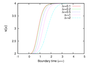
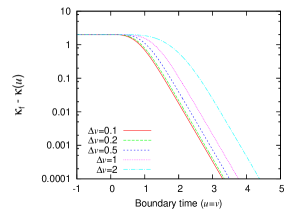
Figure 1: $\kappa(u)$ as a function of time ($u=v$) at the boundary (left) and behaviors of $\kappa(u)$ near the final temperature $\kappa_{\mathrm{f}}$ (right). Time scales of injection are taken to be $\Delta v=0.1,0.2,0.5,1,2$, which are shorter than a typical time scale given by temperature. We set $m_{0}=1/2$ and $\Delta m=15/2$, which give $\kappa_{\mathrm{i}}=2$ and $\kappa_{\mathrm{f}}=4$, respectively.

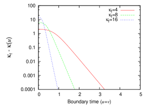
Figure 2: Relaxation rate for final temperatures $\kappa_{\mathrm{f}}=4,8,16$ for the case of null shell accretion ($\Delta v=0$). The initial temperature is given by $\kappa_{\mathrm{i}}=2$. In any case, an exponential decay phase starts after a transient phase, and the decay rate in the exponential decay phase is proportional to inverse of the final temperature.

As the injection time becomes longer than the thermal time scale, $\kappa(u)$ begins to show qualitatively new behaviors. In Fig. 3, for $\Delta v=0,2,10,50$ we plot $\kappa(u)$ together with a quasistatic temperature $2\pi T_{\mathrm{qs}}=2\left(2m(v)\right)^{1/4}$, which is naively determined from the mass functions $m(v)$ in a similar manner to static black holes. We can observe that both curves begin to coincide as the injection time becomes longer. In other words, the variation of the temperature $\kappa(u)$ tends to follow the variation of the black hole mass $m(v)$.

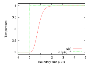
(a) $\Delta v=0$

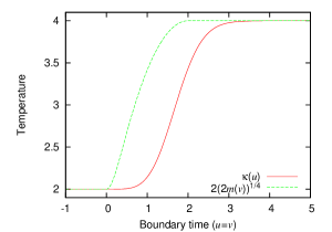
(b) $\Delta v=2$

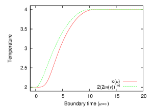
(c) $\Delta v=10$

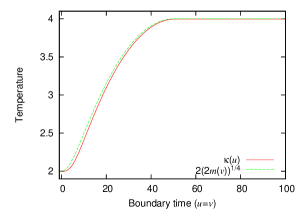
(d) $\Delta v=50$

Figure 3: $\kappa(u)$ and a quasistatic temperature $2\pi T_{\mathrm{qs}}=2(2m(v))^{1/4}$ for various injection times $\Delta v$.

These results lead us to the conclusion that, even if the mass injection is rapid, the temperature will gradually change over a time scale no shorter than the thermal time scale $\sim\kappa^{-1}$. In this sense, we may say that there is a finite relaxation time irrespective of the speed of energy injection. When energy injection and the resultant black hole evolution is slower than this relaxation time, the temperature tends to evolve in a similar way to the mass injection.

IV Summary and Discussion

In this paper we have discussed Hawking temperature for nonstationary spacetimes. We introduced a useful measure for time evolution of spacetime, and showed that the Hawking temperature at each time is determined by the surface gravity of the past horizon when the time evolution of the spacetime is sufficiently slow. This definition of temperature is quite natural because observers can determine it without using causally inaccessible information, such as the position of the event horizon.

Although we have considered an eternal black hole which has the past horizon, the essential calculation does not change for black hole formation in an asymptotically flat spacetime. In this case we should draw null rays from future null infinity back to the past null infinity instead of the past horizon, and as a result we can reproduce the original derivation of the Hawking radiation. The definition of $\kappa(u)$ is the same as Eq. (16), even though it cannot be interpreted as “surface gravity” and should be understood rather in the context of “peeling properties” of outgoing null geodesics, which was discussed in Barcelo:2010xk . It would be interesting to study the properties of $\kappa(u)$ for black holes in an expanding universe, such as those discussed in Refs. Saida:2007ru ; Kaloper:2010ec , for which the derivation is similar to the case of asymptotically flat spacetime. In the case of asymptotically AdS spacetime, in the Poincaré chart the past horizon, which is the Cauchy horizon, exists even in the pure AdS spacetime. This setup is quite similar to the eternal black hole, and we can naturally interpret $\kappa(u)$ as the “surface gravity” of this past horizon.

In the context of the AdS/CFT correspondence, our results indicate that quantum fluctuation of the boundary CFT is governed by the surface gravity of the past horizon when the bulk is the eternal black hole, namely, the thermal equilibrium state. Particularly, our result can be applied to phenomena discussed in Refs. deBoer:2008gu ; Aharony:2005bm , which are directly related to the Hawking radiation in the bulk. It may be interesting to study its implications further. It would be also interesting to study $\kappa(u)$ in numerical solutions obtained in, e.g., Refs. Chesler:2008hg ; Murata:2010dx ; Garfinkle:2011hm , though in general numerical calculation of $\kappa(u)$ becomes difficult at late time due to exponential pileup of outgoing null geodesics onto the horizon.

It is shown that the change of the Hawking temperature is delayed by thermal time scale compared with the mass injection from the boundary. This behavior can be interpreted as follows: The injected matter falls down into the black hole and changes the geometry in the vicinity of the horizon. After that, the Hawking radiation affected by this change emanates from there and reaches the boundary. This process of infall of the matter and return of the modified radiation will take finite time and, roughly speaking, this is the origin of the delay we observed. From the viewpoint of the boundary theory, this delay time can be interpreted as the relaxation time scale needed to achieve thermal equilibrium after the energy injection.

For planar AdS black holes (namely, large black holes in asymptotically AdS spacetime) the horizon is located relatively near to the AdS boundary. If a black hole evolves sufficiently slower than the delay time, we may neglect its delay. In that case, the quasistatic approximation, such that one synchronizes dynamics of the event or apparent horizon and the boundary in terms of the advanced time and uses quantities associated with the future horizon, might be justified.

What we emphasize is that the “surface gravity” of the past horizon, $\kappa(u)$, is not only a geometrical quantity but also one with a physical meaning in the sense that it governs the thermal spectrum of the Hawking radiation observed by asymptotic observers. Many of thermodynamic properties of black holes, however, tend to be associated with the future event or apparent horizon in the previous works, not with the past horizon. It is open to discussion how these points of view are related to each other. It may be also fruitful to study how $\kappa(u)$ is related to other probes of the black hole spacetime, such as those discussed in Ref. Balasubramanian:2011ur , and how our approach is related to other derivations of the Hawking radiation, such as the tunneling approach.

Appendix A redshift factor

In this appendix we show that $\lambda(u)$ defined by Eq. (52) is the redshift factor for the outgoing null ray. Now, we recall that the two-dimensional part of the metric is given by

$$\mathrm{d}s^{2}=\frac{1}{z^{2}}[-F(\bar{v},z)\mathrm{d}\bar{v}^{2}-2\mathrm{d}\bar{v}\mathrm{d}z],$$ (55)

A coordinate transformation such as $z=z(u,v)$ and $\bar{v}=v$ to the double-null coordinates $(u,v)$ gives us the differential form

$$\mathrm{d}z=\frac{\partial z}{\partial u}\mathrm{d}u+\frac{\partial z}{\partial v}\mathrm{d}v=-\frac{F}{2}(-\lambda\mathrm{d}u+\mathrm{d}v),$$ (56)

where we have defined as $\lambda\equiv-\left.\frac{\partial z}{\partial u}\right/\frac{\partial z}{\partial v}$.

We consider a timelike vector field $\xi^{a}=\partial/\partial\bar{v}$ which characterizes a natural Killing time in stationary regions and also in asymptotic regions near the boundary. Note that frequencies of the Killing modes are defined with respect to this Killing time. By using the $1$-form it is rewritten as

$$\xi_{a}=-\frac{1}{z^{2}}(F\mathrm{d}\bar{v}+\mathrm{d}z).$$ (57)

The tangent vector of outgoing null geodesics is given by

$$l^{a}\equiv\frac{\mathrm{d}}{\mathrm{d}s},$$ (58)

where $s$ is an affine parameter, and then the geodesic equations lead to

$$\frac{\mathrm{d}}{\mathrm{d}s}\frac{\dot{\bar{v}}}{z^{2}}=\frac{\partial F}{\partial z}\frac{{\dot{\bar{v}}}^{2}}{2z^{2}},\qquad\dot{z}=-\frac{F}{2}\dot{\bar{v}},$$ (59)

where the dot denotes the derivative with respect to $s$. We note that the last equation is equivalent to the coordinate condition $\partial z/\partial v=-F/2$ defining the double-null coordinates.

The “Killing energy” $E$ associated with the null geodesics is defined by

$$E\equiv-l^{a}\xi_{a}=\frac{1}{z^{2}}(F\dot{\bar{v}}+\dot{z})=\frac{F}{2}\frac{\dot{\bar{v}}}{z^{2}}.$$ (60)

If $\xi^{a}$ is truly a Killing field, $E$ should be constant along the null geodesics. From the geodesic equations we have

$$\frac{\mathrm{d}}{\mathrm{d}\bar{v}}\frac{\dot{\bar{v}}}{z^{2}}=\frac{1}{2}\frac{\partial F}{\partial z}\frac{\dot{\bar{v}}}{z^{2}},$$ (61)

where we have used $\mathrm{d}/\mathrm{d}s=\dot{\bar{v}}\,\mathrm{d}/\mathrm{d}\bar{v}$. On the other hand, differentiating $\partial z/\partial v=-F/2$ with respect to $u$, we have

$$\frac{\partial}{\partial v}\frac{\partial z}{\partial u}=-\frac{1}{2}\frac{\partial F}{\partial z}\frac{\partial z}{\partial u}.$$ (62)

As a result, we find

$$\frac{\partial z}{\partial u}=C\frac{z^{2}}{\dot{\bar{v}}},$$ (63)

where $C$ is an integration constant which can be absorbed into normalization of the affine parameter. Then, the “Killing energy” can be rewritten as

$$E=-C\frac{\partial z}{\partial v}\left/\frac{\partial z}{\partial u}\right..$$ (64)

Since the boundary conditions at $z=0$ are given by

$$\left.\frac{\partial z}{\partial v}\right|_{z=0}=-\left.\frac{\partial z}{\partial u}\right|_{z=0}=-\frac{1}{2},$$ (65)

we have $E_{\mathrm{b}}=C$, which is the energy observed at the boundary, and

$$E|_{z=z(s)}=E_{\mathrm{b}}/\lambda.$$ (66)

Using the geodesic equations, we also have

$$\frac{\mathrm{d}E}{\mathrm{d}s}=\frac{F}{2}\frac{\partial F}{\partial z}\frac{{\dot{\bar{v}}}^{2}}{2z^{2}}+\frac{\dot{\bar{v}}}{2z^{2}}\frac{\mathrm{d}F}{\mathrm{d}s}=\frac{\dot{\bar{v}}}{2z^{2}}\dot{\bar{v}}\frac{\partial F}{\partial\bar{v}}=E\dot{\bar{v}}\frac{\partial\ln F}{\partial\bar{v}}.$$ (67)

Integrating it along the outgoing null geodesics described by $z=z_{\mathrm{g}}(\bar{v})$, we obtain

$$E_{\mathrm{b}}=E_{\mathrm{i}}\exp\int_{\bar{v}_{\mathrm{i}}}^{\bar{v}_{\mathrm{b}}}\mathrm{d}\bar{v}\left(\frac{\partial\ln F}{\partial\bar{v}}\right)_{z=z_{\mathrm{g}}(\bar{v})},$$ (68)

where $E_{\mathrm{i}}$ and $E_{\mathrm{b}}$ are the Killing energy observed at an initial surface and the boundary, respectively.

Consequently, for the outgoing null ray described by $u=\mathrm{const.}$, we have the redshift factor from an initial time $\bar{v}_{\mathrm{i}}$ to asymptotic time $u=\bar{v}_{\mathrm{b}}$ as

$$\lambda(u)=\exp\int_{\bar{v}_{\mathrm{i}}}^{u}\mathrm{d}\bar{v}\left(\frac{\partial\ln F}{\partial\bar{v}}\right)_{z=z_{\mathrm{g}}(\bar{v})}.$$ (69)

It turns out that if the spacetime is stationary, namely, $F$ does not depend on $\bar{v}$, we have $\lambda=1$. The redshift factor $\lambda(u)$ deviates from the unity when time dependence is turned on.

References

- (1) S. W. Hawking, Commun. Math. Phys. 43, 199-220 (1975).
- (2) J. M. Maldacena, Adv. Theor. Math. Phys. 2, 231 (1998) [Int. J. Theor. Phys. 38, 1113 (1999)] [arXiv:hep-th/9711200].
- (3) E. Witten, Adv. Theor. Math. Phys. 2, 505 (1998) [arXiv:hep-th/9803131].
- (4) T. Harada, H. Iguchi and K. i. Nakao, Phys. Rev. D 62, 084037 (2000) [arXiv:gr-qc/0005114].
- (5) H. Saida, T. Harada and H. Maeda, Class. Quant. Grav. 24, 4711 (2007) [arXiv:0705.4012 [gr-qc]].
- (6) A. B. Nielsen, J. H. Yoon, Class. Quant. Grav. 25, 085010 (2008). [arXiv:0711.1445 [gr-qc]].
- (7) S. A. Hayward, R. Di Criscienzo, L. Vanzo, M. Nadalini and S. Zerbini, Class. Quant. Grav. 26, 062001 (2009) [arXiv:0806.0014 [gr-qc]].
- (8) C. Barcelo, S. Liberati, S. Sonego and M. Visser, Phys. Rev. D 83, 041501 (2011) [arXiv:1011.5593 [gr-qc]].
- (9) C. Barcelo, S. Liberati, S. Sonego and M. Visser, JHEP 1102, 003 (2011) [arXiv:1011.5911 [gr-qc]].
- (10) N. Mazumder, R. Biswas and S. Chakraborty, arXiv:1106.4375 [gr-qc].
- (11) D. T. Son, A. O. Starinets, JHEP 0209, 042 (2002). [hep-th/0205051].
- (12) R. A. Janik, R. B. Peschanski, Phys. Rev. D74, 046007 (2006). [hep-th/0606149].
- (13) S. Kinoshita, S. Mukohyama, S. Nakamura, K. -y. Oda, Prog. Theor. Phys. 121, 121-164 (2009). [arXiv:0807.3797 [hep-th]].
- (14) P. M. Chesler and L. G. Yaffe, Phys. Rev. Lett. 102, 211601 (2009) [arXiv:0812.2053 [hep-th]].
- (15) K. Murata, S. Kinoshita, N. Tanahashi, JHEP 1007, 050 (2010). [arXiv:1005.0633 [hep-th]].
- (16) S. R. Das, T. Nishioka and T. Takayanagi, JHEP 1007, 071 (2010) [arXiv:1005.3348 [hep-th]].
- (17) V. E. Hubeny and M. Rangamani, Adv. High Energy Phys. 2010, 297916 (2010) [arXiv:1006.3675 [hep-th]].
- (18) H. Ebrahim and M. Headrick, arXiv:1010.5443 [hep-th].
- (19) K. Hashimoto, N. Iizuka and T. Oka, Phys. Rev. D 84, 066005 (2011) [arXiv:1012.4463 [hep-th]].
- (20) J. Erdmenger, S. Lin and T. H. Ngo, JHEP 1104, 035 (2011) [arXiv:1101.5505 [hep-th]].
- (21) S. Caron-Huot, P. M. Chesler, D. Teaney, Phys. Rev. D84, 026012 (2011). [arXiv:1102.1073 [hep-th]].
- (22) V. Balasubramanian et al., Phys. Rev. D 84, 026010 (2011) [arXiv:1103.2683 [hep-th]].
- (23) D. Garfinkle, L. A. Pando Zayas, Phys. Rev. D84, 066006 (2011). [arXiv:1106.2339 [hep-th]]; D. Garfinkle, L. A. P. Zayas, D. Reichmann, [arXiv:1110.5823 [hep-th]].
- (24) J. de Boer, V. E. Hubeny, M. Rangamani and M. Shigemori, JHEP 0907, 094 (2009) [arXiv:0812.5112 [hep-th]].
- (25) O. Aharony, S. Minwalla, T. Wiseman, Class. Quant. Grav. 23, 2171-2210 (2006). [hep-th/0507219].
- (26) D. Klemm and L. Vanzo, Phys. Rev. D 58, 104025 (1998) [arXiv:gr-qc/9803061].
- (27) S. Hemming, E. Keski-Vakkuri, Phys. Rev. D64, 044006 (2001). [gr-qc/0005115].
- (28) N. Kaloper, M. Kleban, D. Martin, Phys. Rev. D81, 104044 (2010). [arXiv:1003.4777 [hep-th]].