Observational Constraints on the Normal Branch of a Warped DGP Cosmology

Abstract

We investigate observational constraints on the normal branch of the warped DGP braneworld cosmology by using observational data from Type Ia Supernovae (SNIa), Baryon Acoustic Oscillations (BAO), Cosmic Microwave Background (CMB) and Baryon Gas Mass Fraction of cluster of galaxies. The best fit values of model free parameters are: $\Omega_{m}=0.240^{+0.050}_{-0.130}$ and $\Omega_{r_{c}}=0.000^{+0.014}$ at $1\sigma$ confidence interval by using Gold sample SNIa$+$CMB shift parameter$+$BAO$+$Gas mass fraction of baryons in cluster of galaxies. The results for essence sample SNIa combined with CMB shift parameter, BAO and Baryon Gas mass fraction correspont to: $\Omega_{m}=0.220^{+0.020}_{-0.170}$ and $\Omega_{r_{c}}=0.000^{+0.025}$ at $68.3\%$ confidence interval. We determine the age of the universe by using these best fit values. We also study the effective cosmological dynamics on the brane via an effective equation of state parameter and the deceleration parameter to conclude that an effective phantom-like behavior arises in this scenario.

PACS: 98.80.-k,  98.80.Es,  95.36.+x

1 Introduction

The accelerated expansion of the universe supported by recent observational data [1] is one of the most important discoveries in the last decade for the cosmology community. Within the framework of the general relativity, the acceleration could be associated with the so-called dark energy, whose theoretical nature and origin are still unknown for theorists. Cosmological constant or vacuum energy with an equation of state parameter $\omega=-1$, is the most popular candidate for dark energy but unfortunately, it suffers from some serious problems such as fine-tuning and coincidence problems. Therefore, a number of models containing dynamical dark energy have been proposed as the mechanism for late-time cosmic speed up [2]. Some of them are quintessence, k-essence, phantom scalar field, chaplygin gas models and so on. Another alternative approach to explain the late-time cosmic speed up is modification of the geometric sector of the Einstein field equations leading to modified gravity [3]. In the spirit of modified gravity proposal, the Dvali-Gabadadze-Porrati (DGP) braneworld scenario explains the late-time accelerated expansion in its self-accelerating branch without need to introduce a dark energy component on the brane. In this scenario our universe is a $3$-brane embedded in a higher dimensional flat space-time (bulk). The late-time acceleration is driven on large scales by leakage of gravity from the brane into the bulk ( see for instance [4] and references therein). On small scales, gravity is bound to the brane and general relativity is recovered to a good approximation. Indeed, the DGP model has two types of solutions (corresponding to two possible embedding of brane in the bulk ): the self-accelerating, ($DGP^{(+)}$) branch and the normal, ($DGP^{(-)}$) branch. The ($DGP^{(+)}$) branch however, suffers from some instabilities such as ghosts [5] and cannot describe the early stages of the universe evolution properly. There are some extension of the DGP setup that provide relatively wider parameter spaces with richer phenomenology. One of these models is the warped DGP braneworld (WDGP) [6] which is a unified model of Randall-Sundrum II (RSII) braneworld scenario [7] and the DGP setup. In the RSII braneworld model, gravity modifies in early ( high energy) epoches of the universe evolution. The warped DGP scenario also gives a self-accelerating phase in the brane cosmology. It is important to note that, the self-accelerating branch gives an effective equation of state that never can be less than $-1$ (always non-phantom behavior and therefore no crossing of the phantom divide line). The other branch of this scenario is the normal branch ($DGP^{(-)}$) which doesn’t self-accelerate but requires dark energy or modification of the induced gravity on the brane to explain the late time acceleration. It is possible to realize phantom-like effects (without phantom matter) in this normal branch via screening of the brane cosmological constant at late time [8].

This paper is devoted to explore observational status of the normal branch of the warped DGP braneworld cosmology. Observational constraints in DGP model with and without tension is investigated in Ref. [9]. We impose constraints on the model parameters by using the several recent observations such as distance measurements from type Ia supernovae (SNIa) from the Gold [10] and Essence [11] surveys, the baryon acoustic oscillations (BAO) measurement from the large-scale correlation function of the Sloan Digital Sky Survey (SDSS) [12], the position of the first peak of the cosmic microwave background (CMB) from WMAP7 [13] and the baryon gas mass fraction of cluster of galaxies [14]. The structure of the paper is as follows: in section $2$, we introduce the model and its cosmological implications. In sec. $3$ we explore the effect of the WDGP model on the geometrical parameters of the universe. Section $4$ includes the observational constraints on the model parameters space while in section $5$ the detailed results are presented. In section $5$ we perform a detailed comparison between age of the oldest objects of the universe and the age result that obtained from the best fit values of our model parameter space. We also study the effective dynamics of the model in this section. Finally section $6$ is devoted to the concluding remarks.

2 The Model

The action of the warped DGP braneworld model can be written as follows [6,15]

$${\cal{S}}={\cal{S}}_{bulk}+{\cal{S}}_{brane},$$ (1)

$${\cal{S}}=\int_{bulk}d^{5}X\sqrt{-{}^{(5)}g}\bigg{[}\frac{1}{2\kappa_{5}^{2}}{}^{(5)}R+{}^{(5)}{\cal{L}}_{m}\bigg{]}+$$

$$\int_{brane}d^{4}x\sqrt{-g}\bigg{[}\frac{1}{\kappa_{5}^{2}}K^{\pm}+{\cal{L}}_{brane}(g_{\alpha\beta},\psi)\bigg{]}.$$ (2)

Here ${\cal{S}}_{bulk}$ is the action of the bulk, ${\cal{S}}_{brane}$ is the action of the brane and ${\cal{S}}$ is the total action. $X^{A}$ with $A=0,1,2,3,5$ are coordinates in the bulk, while $x^{\mu}$ with $\mu=0,1,2,3$ are induced coordinates on the brane. $\kappa_{5}^{2}$ is 5-dimensional gravitational constant. ${}^{(5)}R$ and ${}^{(5)}{\cal{L}}_{m}$ are 5-dimensional Ricci scalar and matter Lagrangian respectively. $K^{\pm}$ is trace of the extrinsic curvature on either sides of the brane. ${\cal{L}}_{brane}(g_{\alpha\beta},\psi)$ is the effective 4-dimensional Lagrangian. The action ${\cal{S}}$ is actually a combination of the Randall-Sundrum II and the DGP model. In other words, an induced curvature term is appeared on the brane in the Randall-Sundrum II model. Now we consider the brane Lagrangian as follows

$${\cal{L}}_{brane}(g_{\alpha\beta},\psi)=\frac{\mu^{2}}{2}R-\lambda+L_{m},$$ (3)

where $\mu$ is a mass parameter, $R$ is the Ricci scalar of the brane, $\lambda$ is the tension of the brane and $L_{m}$ is the Lagrangian of the other matter fields localized on the brane. We assume that bulk contains only a negative cosmological constant, $\Lambda_{5}$. With these choices, action (1) gives either a generalized DGP or a generalized RS II model: it gives DGP model if $\lambda=0$ and $\Lambda_{5}=0$, and gives RS II model if $\mu=0$. The generalized Friedmann equation on the brane is as follows [6]

$$H^{2}+\frac{k}{a^{2}}=\frac{1}{3\mu^{2}}\bigg{[}\rho+\rho_{0}\Big{(}1+\varepsilon{\cal{A}}(\rho,a)\Big{)}\bigg{]},$$ (4)

where $\varepsilon=\pm 1$ is corresponding to two possible branches of solutions (two different embedding of the brane) in this warped DGP model and ${\cal{A}}=\bigg{[}{\cal{A}}_{0}^{2}+\frac{2\eta}{\rho_{0}}\Big{(}\rho-\mu^{2}\frac{{\cal{E}}_{0}}{a^{4}}\Big{)}\bigg{]}^{1/2}$ where    ${\cal{A}}_{0}\equiv\bigg{[}1-2\eta\frac{\mu^{2}\Lambda_{5}}{\rho_{0}}\bigg{]}^{1/2}$,   $\eta\equiv\frac{6m_{5}^{6}}{\rho_{0}\mu^{2}}$   with $0<\eta\leq 1$   and   $\rho_{0}\equiv m_{\lambda}^{4}+6\frac{m_{5}^{6}}{\mu^{2}}$.  By definition, $m_{\lambda}=\lambda^{1/4}$ and $m_{5}=k_{5}^{-2/3}$.  Also, ${\cal{E}}_{0}$ is an integration constant and corresponding term in the generalized Friedmann equation is called dark radiation term. We neglect dark radiation term in what follows. In this case, the generalized Friedmann equation (4) takes the following form

$$H^{2}+\frac{k}{a^{2}}=\frac{1}{3\mu^{2}}\bigg{[}\rho+\rho_{0}+\varepsilon\rho_{0}\Big{(}{\cal{A}}_{0}^{2}+\frac{2\eta\rho}{\rho_{0}}\Big{)}^{1/2}\bigg{]},$$ (5)

where $\rho\equiv\rho_{m}$ is the energy density of dark matter on the brane.

2.1 Cosmological Implications

In this section we study cosmological dynamics on the DGP brane embedded in a warped bulk Manifold. To this end, we assume a flat FRW universe on the warped DGP brane. In this setup we can rewrite equation (5) as follows

$$H^{2}=\frac{\rho+\lambda}{3\mu^{2}}+\frac{1}{2r_{c}^{2}}\bigg{[}1\pm\sqrt{1+4r_{c}^{2}\Big{(}\frac{\rho+\lambda}{3\mu^{2}}-\frac{{}\Lambda_{5}}{3}\Big{)}}\bigg{]}$$ (6)

where $r_{c}=\frac{m_{4}^{2}}{2m_{5}^{3}}$ is the DGP crossover scale. In the distance scale lower than this scale, gravity behaves as usual general relativistic one but in the distance scales higher than the crossover scale, gravity leaks to the extra dimension and this leakage leads to weakness of gravity in the large scales, so the universe expansion accelerates. The upper sign in equation (6) corresponds to the self-accelerating branch of the model. Taking the lower sign of this equation results a very interesting feature. Indeed, if we assume a model universe with standard cold dark matter (SCDM) with $\rho_{m}=\rho_{0_{m}}\Big{(}\frac{a_{0}}{a}\Big{)}^{3}$ the accelerating behavior of the model can be recovered by rewriting Friedmann equation (6) as follows

$$H^{2}=\frac{\rho_{0_{m}}a_{0}^{3}}{3\mu^{2}a^{3}}+\Lambda_{eff}\,,$$ (7)

where $\Lambda_{eff}$ mimics the role of an effective cosmological constant on the brane (note that it is not actually a constant!) and it can be decomposed into two parts as follows

$$\Lambda_{eff}=\bigg{(}\frac{\lambda}{3\mu^{2}}+\frac{1}{2r_{c}^{2}}\bigg{)}-$$

$$\frac{1}{2r_{c}^{2}}\sqrt{1+4r_{c}^{2}\bigg{(}\frac{\rho_{0}a_{0}^{3}}{3\mu^{2}a^{3}}+\frac{\lambda}{3\mu^{2}}-\frac{{}\Lambda_{5}}{3}\bigg{)}}$$ (8)

The first two terms appeared in parenthesis on the right hand side of this relation could be considered collectively as a cosmological constant term on the brane and the last term on the right hand side (the square root) screens the effect of the brane cosmological constant in the same way as has been pointed out by Lue and Starkman [8]. In this situation, the effective cosmological constant $\Lambda_{eff}$ on the brane increases with time due to dynamical screening effect, that is, reduction of the second term on the right hand side of (8) with cosmic time. In fact the normal branch of the model has the key property that brane is extrinsically curved so that shortcuts through the bulk allow gravity to screen the effects of the brane energy-momentum contents at Hubble parameters $H\sim r_{c}^{-1}$. The screening effect is a result of leakage of gravity to the extra dimension at late times.
For future purposes, it is useful to express the Friedmann equation (6) in a dimensionless form as follows

$$E^{2}(z)=\frac{H^{2}(z)}{H_{0}^{2}}=\Omega_{m}(1+z)^{3}+\Omega_{\lambda}+2\Omega_{r_{c}}-$$

$$2\sqrt{\Omega_{r_{c}}}\sqrt{\Omega_{m}(1+z)^{3}+\Omega_{\lambda}+\Omega_{r_{c}}+\Omega_{\Lambda_{5}}}$$ (9)

where $\Omega_{m}=\frac{\rho_{0m}}{3\mu^{2}H_{0}^{2}}$  ,  $\Omega_{\lambda}=\frac{\lambda}{3\mu^{2}H_{0}^{2}}$  ,  $\Omega_{r_{c}}=\frac{1}{4r_{c}^{2}H_{0}^{2}}$  $\Omega_{{}\Lambda_{5}}=\frac{-\Lambda_{5}}{3H_{0}^{2}}$ and $H_{0}=100h\quad km/s/Mpc$. Taking $z=0$ imposes a constraints on the model parameters as follows

$$\Omega_{m}+\Omega_{\lambda}+2\Omega_{r_{c}}-2\sqrt{\Omega_{r_{c}}}\sqrt{\Omega_{m}+\Omega_{\lambda}+\Omega_{r_{c}}+\Omega_{{}\Lambda_{5}}}=1\,.$$ (10)

The general relativistic limit can be recovered if we set $\Omega_{r_{c}}=0$ (or $m_{5}=0$). In this case equations (10) implies that $\Omega_{m}+\Omega_{\lambda}=1$. Considering the tension of the brane as a cosmological constant this case leads to the $\Lambda$CDM cosmology.

3 The effect of WDGP on the Geometrical Parameters of the Universe

The cosmological observations are mainly dependent on the background geometry ( especially background spatial curvature) of the universe. So, in this section we study the effect of the WDGP model on the geometrical parameters of the universe.

1. Comoving radial Distance

One of the basic parameters in cosmology is the comoving radial distance. For an object with redshift $z$ in a FRW background, this parameter can be expressed as follows

$$r(z)=\frac{c}{H_{0}\sqrt{|\Omega_{K}|}}{\cal{F}}\Big{(}\sqrt{|\Omega_{K}|}\int_{0}^{z}\frac{dz^{\prime}}{H(z^{\prime})/H_{0}}\Big{)}\,,$$ (11)

where ${\cal{F}}\equiv(x,\,\sin x,\,\sinh x)$  for $K=(0,\,1,\,-1)$  respectively.  $K$ marks curvature of the spatial geometry and $\Omega_{K}=\frac{K}{3\mu^{2}H_{0}^{2}}$. Figure $1$ shows the radial comoving distance versus the redshift for different values of $\Omega_{{r}_{c}}$ in a flat background. Clearly, increasing the values of $\Omega_{r_{c}}$ results in a longer comoving distance. The mentioned quantity is a useful quantity in the analysis of the luminosity distances of Supernova type Ia.

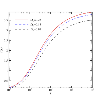
Figure 1: Comoving radial distance versus the redshift for different values of $\Omega_{{r}_{c}}$ in a flat FRW universe. The unit of vertical axis is $c/H_{0}$.

2. Angular size

The apparent angular size of an object located at the cosmological distance is another important parameter that can be affected by the cosmological model during the history of the universe. If we take the object to lie perpendicular to the line of sight and to have physical extent $D$, the apparent angular size $\theta$ is given by

$$\theta=\frac{D}{d_{A}(z)}$$ (12)

where $d_{A}(z)=r(z)/(1+z)$ is the angular diameter distance which is a measure of how large objects appear to be in the universe. A key application of equation (12) is in the study of features of the cosmic microwave background radiation. The variation of apparent angular size $\Delta\theta$ in terms of the $\Delta z$ is given by

$$\frac{\Delta z}{\Delta\theta}=H(z)r(z).$$ (13)

This relation is the so-called Alcock-Paczynski test. The advantage of the Alcock-Paczynski test is that in this case, instead of using a standard candle, we use a standard ruler such as the baryonic acoustic oscillation. Figure $2$ shows $\Delta z/\Delta\theta$ for different values of $\Omega_{{r}_{c}}$ in a flat FRW background. As the figure shows, increasing of $\Omega_{{r}_{c}}$ results in larger values of $\Delta z/\Delta\theta$.

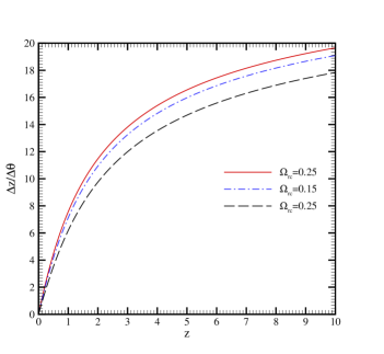
Figure 2: $\Delta z/\Delta\theta$ versus the redshift for different values of $\Omega_{{r}_{c}}$ in a flat FRW background.

3. Comoving Volume Element

The comoving volume element is another geometrical parameter which is used in number-count tests such as lensed quasars, galaxies, or clusters of galaxies. The comoving volume element can be expressed in terms of comoving distance and Hubble parameter as follows

$$f=\frac{dV}{dzd\Omega}=\frac{r^{2}(z)}{H(z)}\,.$$ (14)

Figure $3$ shows the comoving volume element versus the redshift for different values of $\Omega_{{r}_{c}}$ in a flat FRW background. This figure indicates that the value of the comoving volume element increases with the increasing of $\Omega_{{r}_{c}}$. We note the quantities displayed in figures 1-3 are specified just by giving the value of $\Omega_{{r}_{c}}$ alone. This is because we are interested in the DGP character of the model. Nevertheless, in plotting these figures we have used the values $\Omega_{m}=0.24$, $\Omega_{{\Lambda}_{5}}=1$ and the other quantity $\Omega_{\lambda}$ is obtained via constraint equation, (10).

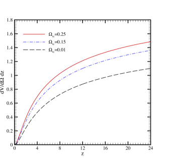
Figure 3: Comoving volume element versus the redshift for different values of $\Omega_{{r}_{c}}$ in a flat FRW background.

4 Observational Constraints

In this section, we constrain the model parameters of the warped DGP scenario by using the most recent observational data including the SNIa data measurements as given by the gold and essence samples, combined with the information from the BAO measurements by SDSS, the CMB shift parameter from WMAP7 observations and the baryon gas mass fraction.

A: SNIa data

Here we use some new sample supernova type Ia data such as the gold sample compiled in [10] and essence sample compiled in [11] to constrain the free parameters of the model. This observation directly measures the apparent magnitude $m$ of a supernova versus its redshift $z$. We note that deference between SNIa samples is in their systematic errors and the range of redshift which the apparent magnitude is determined .

The theoretical distance modulus is defined as

$$\mu=m-M=5\log_{10}d_{L}+5\log_{10}\left(\frac{c/H_{0}}{1\quad Mpc}\right)+25,$$ (15)

where $M$ is the absolute magnitude that is believed to be constant for all Type Ia supernovae and $d_{L}$ is the luminosity distance that in general case can be expressed as follows

$$d_{L}(z;\{\theta_{i}\})=\frac{(1+z)}{\sqrt{|\Omega_{K}|}}{\cal{F}}\left(\sqrt{|\Omega_{K}|}\int_{0}^{z}\frac{dz^{\prime}}{E(z^{\prime};\{\theta_{i}\})}\right)$$ (16)

where $\{\theta_{i}\}$ denotes the model parameters and $E(z)$ is given by equation (9). We estimate the best fit of the set of parameters $\{\theta_{i}\}$ by using a $\chi^{2}$ statistics, with

$$\chi^{2}_{SN}(\{\theta_{i}\})=\sum_{j=1}^{N}\frac{[\mu_{obs}(z_{j};\{\theta_{i}\})-\mu_{th}(z_{j};\{\theta_{i}\})]^{2}}{\sigma_{j}^{2}},$$ (17)

In this relation, $N$ is the number of SNIa data points which is different in several data sets, $\mu_{obs}$ is the observed distance modulus and the $\sigma_{j}$ is the uncertainty in the observed distance modulus, which is assumed to be Gaussian and uncorrelated so that the likelihood is proportional to   $\exp(-\chi^{2}/2)$. The parameter $\overline{M}=5\log_{10}\big{(}\frac{c/H_{0}}{1\quad Mpc}\big{)}+25$ is a nuisance parameter and it is independent of the data and the data sets. Following the techniques described in Ref. [16], the minimization with respect to $\overline{M}$ can be made by expanding the $\chi^{2}_{SN}$ of equation (17) with respect to $\overline{M}$ as

$$\chi^{2}_{SN}(\{\theta_{i}\})=\tilde{A}-2M\tilde{B}+M^{2}\tilde{C}$$ (18)

where

$$\tilde{A}(\{\theta_{i}\})=\sum_{j=1}^{N}\frac{[\mu_{obs}(z_{j};\{\theta_{i}\})-\mu_{th}(z_{j};\{\theta_{i}\},M=0)]^{2}}{\sigma_{j}^{2}},$$ (19)

and

$$\tilde{B}(\{\theta_{i}\})=\sum_{j=1}^{N}\frac{\mu_{obs}(z_{j};\{\theta_{i}\})-\mu_{th}(z_{j};\{\theta_{i}\},M=0)}{\sigma_{j}^{2}}$$

$$,\quad\quad\tilde{C}=\sum_{j=1}^{N}\frac{1}{\sigma_{j}^{2}}.$$ (20)

Equation (18) has a minimum for $M=\frac{\tilde{B}}{\tilde{C}}$   at  $\tilde{\chi}^{2}_{SN}(\{\theta_{i}\})=\tilde{A}(\{\theta_{i}\})-\frac{\tilde{B}^{2}(\{\theta_{i}\})}{\tilde{C}}$. Using this equation the best fit values of model parameters as the values that minimize $\chi^{2}_{SNIa}(\{\theta_{i}\})$ can be obtained.

For the likelihood analysis we marginalize the likelihood function $L\sim\exp(-\chi^{2}/2)$ over $h$. We adopted Gaussian priors such that $h=0.705$ from the WMAP7 [13]. Table $1$ summarizes these priors.

Table 1: Priors on the parameter space used in the likelihood analysis.

Parameter	Prior
$\Omega_{m}$	0.000  -   1.000  Top Hat
$\Omega_{r_{c}}$	0.000  -   1.000  Top Hat
$\Omega_{\Lambda_{5}}$	-1.000  -  1.000  Top Hat
$h$	-   -

B: CMB shift parameter

We use the CMB data from WMAP7 observation that includes the shift parameter $\cal{R}$ and the redshift of the decoupling epoch $z_{*}$. The shift parameter $\cal{R}$ relates the angular diameter distance to the last scattering surface, the comoving size of the sound horizon at $z_{*}=1091.3$ and the angular scale of the first acoustic peak in the CMB power spectrum of the temperature fluctuations. The CMB shift parameter is approximated by (see for more details Ref. [16])

$${\cal{R}}=\frac{\sqrt{\Omega_{m}}H_{0}}{c}(1+z_{*})d_{A}(z_{*}),$$ (21)

where $d_{A}(z)$ is the angular diameter distance defined by equation (12). The constraints on a typical model using CMB shift is obtained from minimization of the quantity

$$\chi^{2}_{CMB}=\frac{[{\cal{R}}_{obs}-{\cal{R}}_{th}]^{2}}{\sigma_{CMB}^{2}},$$ (22)

where ${\cal{R}}_{obs}=1.725$ is the observed value of the CMB shift parameter performed from WMAP7 observation and its corresponding $1\sigma$ error is $\sigma_{CMB}=0.018$ [13]. Also ${\cal{R}}_{th}$ corresponds to the theoretical value of shift parameter calculated from equation (21).

C: BAO observation

The baryonic acoustic oscillation (BAO) peak detected in the SDSS luminous red Galaxies (LRG) is another tool to test the model against observational data. BAO are described in terms of a dimensionless parameter

$${\cal{A}}(z_{sdss};\{\theta_{i}\})=\sqrt{\Omega_{m}}\bigg{[}\frac{H_{0}d_{L}^{2}(z_{sdss};\{\theta_{i}\})}{H(z_{sdss};\{\theta_{i}\})z_{sdss}^{2}(1+z_{sdss})^{2}}\bigg{]}^{1/3}\,.$$ (23)

The $\chi^{2}$ for the BAO is given by

$$\chi^{2}_{sdss}=\frac{[{\cal{A}}_{obs}-{\cal{A}}_{th}]^{2}}{\sigma_{sdss}^{2}}.$$ (24)

The observed value ${\cal{A}}_{obs}$ from the LRG is ${\cal{A}}_{obs}=0.469\Big{(}\frac{n_{s}}{0.98}\Big{)}^{-0.35}\pm 0.017$ measured at $z_{sdss}=0.35$ [20]. Here $n_{s}=0.963$ is the spectral index as measured by WMAP seven years observations [13].

D: Gas mass fraction of cluster of galaxies

Another cosmological test to constrain the parameters of the model arises from baryon gas mass fraction of cluster of galaxies for a range of redshifts

$$f_{gas}=\frac{M_{gas}}{M_{tot}}\,.$$ (25)

The basic assumption underlying this method is that the baryon gas mass fraction in clusters is constant, independent of redshift. This method can give a constraint to the geometry of the universe with the relation ${\cal{S}}_{gas}\propto d_{A}^{\frac{3}{2}}$ under the assumption that this fraction should be approximately constant with redshift. Following [17] (see also [16]), the $\chi^{2}$ expression for gas mass fraction is given by

$$\chi^{2}_{gas}(\{\theta_{i}\})=\sum_{j}\frac{[{\cal{S}}_{gas}^{obs}(z_{j};\{\theta_{i}\})-{\cal{S}}_{gas}^{th}(z_{j};\{\theta_{i}\})]^{2}}{\sigma_{j}^{2}},$$ (26)

where ${\cal{S}}_{gas}$ is a dimensionless parameter defined as

$${\cal{S}}_{gas}=\frac{b}{1+\beta}\frac{\Omega_{b}}{\Omega_{m}}\bigg{(}\frac{d_{A}^{flat}(z)}{d_{A}(z)}\bigg{)}^{\frac{3}{2}}.$$ (27)

In this relation $d_{A}^{flat}$ is the angular diameter distance to a cluster in the test model which is assumed to be SCDM (cold dark matter) in this case, and $b$ is a bias factor suggesting that the baryon fraction in clusters is slightly lower than for the universe as a whole. Also $1+\beta$ is a factor taking into account the fact that the total baryonic mass in clusters consists of both X-ray gas and optically luminous baryonic mass (stars), the latter being proportional to the former with proportionality constant $\beta\simeq 0.19\sqrt{h}$ [16-18]. The nuisance parameter $\xi=\frac{b}{1+\beta}\frac{\Omega_{b}}{\Omega_{m}}$ should be marginalized via expanding the $\chi^{2}_{gas}$ of equation (26) with respect to $\xi$ which gives

$$\chi^{2}_{gas}=K-\frac{W^{2}}{Y}$$ (28)

where

$$K=\sum_{j}\frac{{\cal{S}}_{gas}^{obs}(z_{j};\{\theta_{i}\})^{2}}{\sigma_{j}^{2}},$$ (29)

and

$$W=\sum_{j}\frac{{\cal{S}}_{gas}^{obs}(z_{j};\{\theta_{i}\}).{\cal{S}}_{gas}^{th}(z_{j};\{\theta_{i}\},\xi=1)}{\sigma_{j}^{2}},$$

$$Y=\sum_{j}\frac{{\cal{S}}_{gas}^{th}(z_{j};\{\theta_{i}\},\xi=1)^{2}}{\sigma_{j}^{2}}.$$ (30)

We use the $26$ cluster data [14] for ${\cal{S}}_{gas}^{obs}$ to obtain the best fit parameters of the model.

It is important to note that the above observational data are uncorrelated since they are given by different experiments and methods. So, we can construct a joint analysis as

$$\chi^{2}_{tot}=\chi^{2}_{SN}+\chi^{2}_{CMB}+\chi^{2}_{SDSS}+\chi^{2}_{gas}\,\,.$$ (31)

5 Results

With these preliminaries, we have obtained the best fit parameters of the normal branch of the WDGP model for SNIa data (gold and essence datasets), the joint analysis of the SNIa and CMB, the combined analysis of the SNIa, CMB and SDSS and finally the joint analysis of the total datasets including cluster galaxies gas mass fraction. Table $2$ shows the results of the observational constraints on the free parameters of this model. Figure $4$ shows the marginalized relative likelihood with respect to parameter $\Omega_{m}$ and $\Omega_{r_{c}}$ fitted with SNIa gold sample, SNIa+CMB,  SNIa+CMB+SDSS experiments and SNIa+CMB+SDSS+gas mass fraction observations. In figure $5$, we repeat these stages for Essence sample of SNIa experiments together with other data sets. We plot contour maps of $\Omega_{r_{c}}$ versus $\Omega_{m}$ in figure $6$ for Gold Sample and combined observational data sets. In figure $7$ we plot corresponding contour maps for Essence Sample and combined observational data sets.

Table 2: The fitting results for WDGP model by using the SNIa (Gold and Essence Samples), SNIa+CMB and SNIa+CMB+SDSS and SNIa+CMB+SDSS+glaxies clusters gas mass fraction experiments in a flat background.

Observation	$\Omega_{m}$	$\Omega_{r_{c}}$	$\Omega_{\lambda}$	$\Omega_{\Lambda_{5}}$	$\chi^{2}_{min}/N_{d.o.f}$	Age(Gyr)
SNIa( Gold Sample)	$0.030^{+0.220}_{-0.025}$	$0.160^{+0.030}_{-0.150}$	$0.168^{+0.360}_{-0.016}$	0.009	0.923	$64.97^{+42.250}_{-35.855}$
SNIa(Gold)+CMB	$0.280^{+0.050}_{-0.130}$	$0.000^{+0.010}$	$0.631^{+0.204}_{-0.117}$	0.939	0.943	$14.38^{+1.245}_{-3.344}$
SNIa(Gold)+CMB+SDSS	$0.260^{+0.060}_{-0.120}$	$0.000^{+0.012}$	$0.644^{+0.302}_{-0.112}$	0.839	0.992	$14.51^{+1.448}_{-3.128}$
SNIa(Gold)+CMB+SDSS+GAS	$0.240^{+0.050}_{-0.130}$	$0.000^{+0.014}$	$0.660^{+0.174}_{-0.139}$	0.999	0.992	$14.85^{+1.561}_{-3.942}$
SNIa( Essence Sample)	$0.020^{+0.240}_{-0.015}$	$0.170^{+0.020}$	$0.161^{+0.074}_{-0.037}$	0.009	1.032	$78.38^{+56.018}_{-42.390}$
SNIa(Essence)+CMB	$0.230^{+0.020}_{-0.160}$	$0.000^{+0.019}$	$0.691^{+0.133}_{-0.061}$	0.539	1.030	14.86${}^{+1.435}_{-6.392}$
SNIa(Essence)+CMB+SDSS	$0.220^{+0.030}_{-0.190}$	$0.000^{+0.022}$	$0.697^{+0.145}_{-0.095}$	0.689	1.054	15.07${}^{+1.758}_{-6.977}$
SNIa(Essence)+CMB+SDSS+GAS	$0.220^{+0.020}_{-0.170}$	$0.000^{+0.025}$	$0.713^{+0.187}_{-0.125}$	0.119	1.044	$14.96^{+1.459}_{-7.888}$

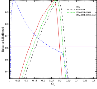
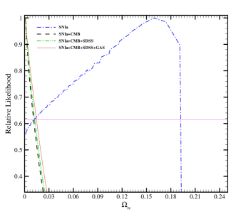
Figure 4: Marginalized relative likelihood with respect to parameter $\Omega_{m}$ (left) and $\Omega_{r_{c}}$ (right) fitted with SNIa Gold Sample, SNIa (Gold)+CMB, SNIa(Gold)+CMB+SDSS and SNIa(Gold)+CMB+SDSS+ galaxies clusters gas mass fraction experiments. The intersection of each curve with horizontal solid line is corresponding to the bound with $1\sigma$ confidence level.

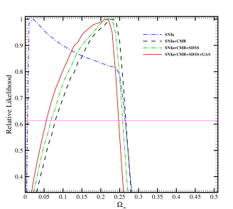
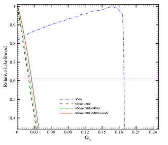
Figure 5: Marginalized relative likelihood with respect to parameter $\Omega_{m}$ (left) and $\Omega_{r_{c}}$ (right) fitted with SNIa Essence sample, SNIa (Essence)+CMB, SNIa (Essence)+CMB+SDSS and SNIa (Essence)+CMB+SDSS+galaxies clusters gas mass fraction experiments. The intersection of each curve with horizontal solid line is corresponding to the bound with $1\sigma$ confidence level.

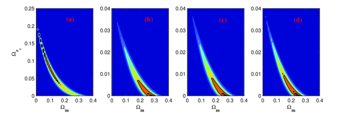
Figure 6: Contour maps of $\Omega_{r_{c}}$ versus $\Omega_{m}$ for WDGP model with $1\sigma\,(68.3\%)$ and $2\sigma\,(95.5\%)$ confidence levels using SNIa (a), SNIa+CMB (b), SNIa+CMB+SDSS (c) and SNIa+CMB+SDSS+Gas (d). We used the Gold Sample for SNIa experiment.

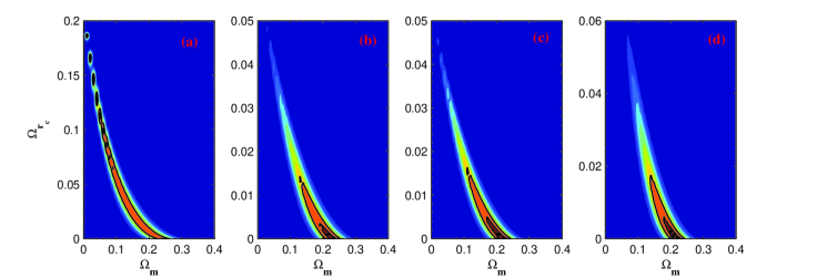
Figure 7: Contour maps of $\Omega_{r_{c}}$ versus $\Omega_{m}$ for normal branch of WDGP model with $1\sigma\,(68.3\%)$ and $2\sigma\,(95.5\%)$ confidence levels using SNIa (a), SNIa+CMB (b), SNIa+CMB+SDSS (c) and SNIa+CMB+SDSS+Gas (d). We used the Essence Sample for SNIa experiment..

5.1 The Age of the universe

The age of the universe for an expanding universe in a flat background is given by

$$t_{0}=\int_{0}^{t_{0}}dt=\int_{0}^{\infty}\frac{dz}{(1+z)H(z)}.$$ (32)

The WMAP collaboration [13],  using the $\Lambda CDM$ model, quotes  $t_{0}=13.75\pm 0.11$ Gyr. In our model $H(z)$ is given by Eq. (9). A model-independent limit of $t_{0}$ can be obtained from the age of the oldest stars, $t_{star}$. Since the age of the universe should be greater than the age of the oldest stars, this limit can be used as another probe to constrain our model ( see for instance [19,20]). Studies on the old stars [21] suggest an age of $13^{+4}_{-2}$ Gyr for the universe. Richer et. al. [22] and Hansen et. al. [23] also proposed an age of $12.7\pm 0.7$ Gyr, using the white dwarf cooling sequence method. Recently, Frebel et al. [24] have reported the discovery of HE $1523-0901$, with an age $t_{star}=13.4\pm 0.8(1\sigma)\pm 1.8(syst)$ Gyr. With these statistical and systematic errors, we adopt $t_{star}>12$ Gyr for constraining our model [21]. Table $2$, shows that the age of the universe is always greater than $t_{star}$ for all used data sets. However, the SNIa data sets (Gold or Essence Samples) alone lead to very great $t_{0}$ which is not reliable and it seems that the pure SNIa test cannot give a good constraint on the model parameters space. This feature is evident also in our previous relative likelihood figures and has its origin in the geometric nature of the SNIa data sets. On the other hand the combined analysis of SNIa with other data sets improves the constraints and gives a more reasonable results.

5.2 Effective Dynamics

It has been shown in our previous work [15] that the Warped DGP scenario has a phantom-like behavior without need to introduce a phantom matter neither in the bulk nor on the brane. To investigate the effective dynamics of the model we study the effective density defined by

$$\rho_{eff}=\lambda+\frac{3\mu^{2}}{2r_{c}^{2}}\bigg{[}1-\sqrt{1+4r_{c}^{2}\Big{(}\frac{\rho+\lambda}{3\mu^{2}}-\frac{{}\Lambda_{5}}{3}\Big{)}}\bigg{]}$$ (33)

and an effective equation of state parameter

$$\omega_{eff}=-1-\frac{\dot{\rho}_{eff}}{3H\rho_{eff}}\,.$$ (34)

So, the effective equation of state of dark energy can be expressed as follows

$$\omega_{eff}=-1+$$

$$\frac{-\Omega_{m}(1+z)^{3}}{\bigg{(}E^{2}-\Omega_{m}(1+z)^{3}\bigg{)}\sqrt{1+\frac{4}{\Omega_{r_{c}}}\Big{(}\Omega_{m}(1+z)^{3}+\Omega_{\lambda}+\Omega_{{}\Lambda_{5}}\Big{)}}}$$ (35)

Using the best fit parameters obtained here and summarized in table $2$,  in figure $8$ we plot $\omega_{eff}$ versus the redshift for combined SNIa+CMB+SDSS+galaxies clusters gas mass fraction data set for Gold and Essence Samples.

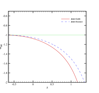
Figure 8: The effective equation of state parameter versus the redshift fitted with SNIa+CMB+SDSS+galaxies clusters gas mass fraction with Gold and Essence Samples respectively.

As the figure shows, in low redshifts and especially at present, dark energy exhibits a phantom-like acceleration with $\omega_{eff}<-1$ ( it is easy to show also that in this model $\dot{H}<0$ and $\dot{\rho}_{eff}>0$,  see [15] for details). In future ( $z<0$) the effective equation of state parameter approaches the cosmological constant line $\omega_{eff}=-1$. It is important to note that although $\omega_{eff}$ has a phantom-like dynamics in this warped DGP scenario, $\omega_{tot}$ doesn’t show such a behavior. The expression for $w_{tot}$ is given by

$$\omega_{tot}=-1+$$

$$\frac{\Omega_{m}(1+z)^{3}}{E^{2}}\Bigg{(}1-\sqrt{\frac{\Omega_{r_{c}}}{\Omega_{r_{c}}+\Omega_{m}(1+z)^{3}+\Omega_{\lambda}+\Omega_{{}\Lambda_{5}}}}\Bigg{)}.$$ (36)

Indeed, the total equation of state parameter remains Quintessence-like ($w_{tot}>-1$) as figure $9$ shows.

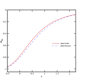
Figure 9: Total equation of state parameter versus the redshift fitted with SNIa+CMB+SDSS+ galaxies clusters Gas mass fraction with Gold and Essence Samples respectively.

Another dynamical quantity of interest is the deceleration parameter which is expressed as $q=-(1+\frac{\dot{E}}{H_{0}E^{2}})$ where

$$\frac{\dot{E}}{H_{0}}=\frac{-3}{2}\Big{(}\Omega_{m}(1+z)^{3}\Big{)}$$

$$\times\Bigg{[}1-\sqrt{\frac{\Omega_{r_{c}}}{\Omega_{r_{c}}+\Omega_{m}(1+z)^{3}+\Omega_{\lambda}+\Omega_{{}\Lambda_{5}}}}\Bigg{]}.$$ (37)

This equation implies that for all values of $z$,  $\dot{E}<0$. As an important result, the deceleration parameter could be never less than $-1$. Consequently, there is no super-acceleration or big rip singularity in this model. Figure $10$ shows the variation of the deceleration parameter versus the redshift with two combined data sets. It is clear that the deceleration parameter reduces by redshift towards recent epoch and in the future it approaches $q=-1$.

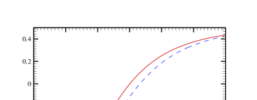
Figure 10: Variation of the deceleration parameter versus the redshift. The parameters values used to produce this figure are taken from table $2$.

6 Summary and Conclusion

The normal branch of the warped DGP brane scenario has several fascinating properties. Its cosmological dynamics does not suffer from instabilities such as ghost, it can exhibit a phantom mimicry and it leads to the famous $\Lambda$CDM scenario in certain limits. In this regard, we have studied cosmological constraints imposed on this model from observational data such as type Ia supernova data from the Gold and Essence surveys, the baryon acoustic oscillations (BAO) measurement from the Sloan Digital Sky Survey (SDSS), the cosmic microwave background (CMB) and the baryon gas mass fraction of clusters of galaxies. We find that the best fit values of model free parameters are constrained to: $\Omega_{m}=0.240^{+0.050}_{-0.130}$ and $\Omega_{r_{c}}=0.000^{+0.014}$ at $1\sigma$ confidence interval by using Gold sample SNIa $+$ CMB shift parameter $+$ BAO $+$ gas mass fraction. The same analysis just including essence sample SNIa instead of Gold sample correspond to: $\Omega_{m}=0.220^{+0.020}_{-0.170}$ and $\Omega_{r_{c}}=0.000^{+0.025}$ at $68\%$ confidence interval. Furthermore, using these best fit parameters, we obtained the age of the universe $14.85^{+1.561}_{-3.942}$ and $14.96^{+1.459}_{-7.888}$ at $1\sigma$ confidence interval by using SNIa$+$CMB shift parameter$+$BAO$+$gas mass fraction for gold sample and essence sample of SNIa respectively. A comparison between the age of the oldest stars and the one that we have obtained by using the best fit values of parameters, show that WDGP passes the age constraint very well. On the other hand we investigated the effect of the WDGP model on the geometrical parameters of the universe such as the transverse comoving distance (comoving angular diameter distance), the comoving volume element and the angular size. And finally, we studied the effective cosmological dynamics of the model via effective equation of state parameter and the deceleration parameter by using the best fit parameters of the combined analysis of SNIa+CMB+SDSS+galaxies clusters gas mass fraction with Gold and Essence Samples. This analysis confirms that the WDGP model has a phantom-like behavior without need to introduce phantom fields neither in the bulk nor on the brane. It is important to note that in this scenario the effect of the bulk’s warped geometry (encoding in $\Lambda_{5}$) is that by increasing the absolute value of the bulk cosmological constant the phantom-like behavior reduces. In other words, incorporation of $\Lambda_{5}$ leads to a reduction of the effective phantom nature of the model in comparison with pure DGP case ( see Ref. [15]).

References

-
(1)
A. G. Riess et al, Astrophys. J. 607 (2004) 665
S. P. Boughn, and R.G. Crittenden, Mon. Not. R. Astron. Soc. 360 (2005) 1013
V. Springel, C. S. Frenk, and S. M. D. White, Nature (London) 440 (2006) 1137
D. N. Spergel et al, Astrophys. J. Suppl. 170 (2007) 377. -
(2)
E. J. Copeland, M. Sami and S. Tsujikawa, Int. J. Mod. Phys. D
15 (2006) 1753
D. T. Valentini and L. Amendola, Phys. Rev. D 65 (2002) 063508
R. R. Caldwell, Phys. Lett. B 545 (2002) 23
V. Sahni, Lect. Notes Phys. 653 (2004) 141, [ arXiv:astro-ph/0403324]
V. Sahni and A. Starobinsky, Int. J. Mod. Phys. D 15 (2006) 2105
R. Durrer and R. Maartens, Gen. Rel. Grav. 40 (2008) 301
H. Zhang, [arXiv:0909.3013]
Y. -F. Cai, E. N. Saridakis, M. R. Setare and J. -Q. Xia, Phys. Rep. 493 (2010) 1-60, [arXiv:0909.2776]. -
(3)
S. Nojiri and S. D. Odintsov, Int. J. Geom. Meth. Mod. Phys. 4
(2007) 115
T. P. Sotiriou and V. Faraoni, Rev. Mod. Phys. 82 (2010) 451, [arXiv:0805.1726]
S. Capozziello and M Francaviglia, Gen. Relativ. Gravit. 40 (2008) 357
A. De Felice and S. Tsujikawa, Living Rev. Rel. 13 (2010) 3, [arXiv:1002.4928]
S. Capozziello and V. Salzano, [arXiv:0902.0088]
S. Capozziello, M. De Laurentis and V. Faraoni, [arXiv:0909.4672]. - (4) A. Lue, Phys. Rept. 423 (2006) 1-48.
-
(5)
K. Koyama, Class. Quantum Grav. 24 (2007) R231
C. de Rham and A. J. Tolley, JCAP 0607 (2006) 004. - (6) Kei-ichi Maeda, S. Mizuno and T. Torii, Phys. Rev. D 68 (2003) 024033.
- (7) L. Randall, R. Sundrum, Phys. Rev. Lett. 83 (1999) 4690.
-
(8)
V. Sahni and Y. Shtanov, JCAP 0311 (2003) 014
A. Lue and G. D. Starkman, Phys. Rev. D 70 (2004) 101501
L. P. Chimento, R. Lazkoz, R. Maartens and I. Quiros, JCAP 0609 (2006) 004
R. Lazkoz, R. Maartens and E. Majerotto, Phys. Rev. D 74 (2006) 083510
K. Nozari and M. Pourghassemi, JCAP 10 (2008) 044
M. Bouhmadi-Lopez and P. Vargas Moniz, Phys. Rev. D 78 (2008) 084019, [arXiv:0804.4484]
K. Nozari and F. Kiani, JCAP 07 (2009) 010, [arXiv:0906.3806]
K. Nozari and N. Rashidi, JCAP 0909 (2009) 014
K. Nozari, T. Azizi and M. R. Setare, JCAP 0910 (2009) 022, [arXiv:0910.0611]
M. Bouhmadi-Lopez, JCAP 0911 (2009) 2009, [arXiv:0905.1962]. -
(9)
L. Lombriser, W. Hu, W. Fang and U. Seljak, Phys. Rev. D80
(2009) 063536, [arXiv:0905.1112]
See also
S. Rydbeck, M. Fairbairn and A. Goobar, JCAP 0705 (2007) 003.
R. Maartens and E. Majerotto, Phys. Rev. D74 (2006) 023004. - (10) A. G. Riess et al, Astrophys. J. 659 (2007) 98.
-
(11)
W. M. Wood-Vasey et al, Astrophys. J. 666 (2007) 694,
[arXiv:astro-ph/0701041]
J. Lu, L. Xu, M. Liu and Y. Gui, Eur. Phys. J. C 58 (2008) 311, [arXiv:0812.3209]. - (12) R. Kessler et al, [arXiv:0908.4274].
- (13) E. Komatsu et al, [arXiv:1001.4538].
- (14) S. W. Allen, et al, Mon. Not. Roy. Astron. Soc. 353 (2004) 457.
- (15) K. Nozari and T. Azizi, Commun. Theor. Phys. 54 (2010) 773.
- (16) M. S. Movahed, M. Farhang and S. Rahvar, Int. J. Theor. Phys. 48 (2009) 1203, [arXiv:astro-ph/0701339].
- (17) S. Nesseris and L. Perivolaropoulos, JCAP 0701 (2007) 018, [arxiv:astro-ph/0610092].
- (18) S. Baghram, M. S. Movahed and S. Rahvar, Phys. Rev. D 80 (2009) 064003, [arxiv:0904.4390].
- (19) M. S. Movahed and A. Sheykhi, Mon. Not. R. Astron. Soc. 388 (2008) 197, [arxiv:0707.2199].
- (20) D. J. Eisenstein et al., [arxiv:astro-ph/0501171].
-
(21)
E. Carretta et al., Astrophys. J. 533 (2000) 215
B. Chaboyer and L. M. Krauss, Astrophys. J. Lett. 567 (2002) L45. - (22) H. B. Richer et al., Astrophys. J. 574 (2002) L151.
- (23) B. M. S. Hansen et al., Astrophys. J. 574, (2002) L155.
- (24) A. Frebel et al., Astrophys. J. Lett. 660 (2007) L117.