Detecting Einstein-Podolsky-Rosen steering for continuous variable wavefunctions

Abstract

By use of Reid’s criterion and the entropic criterion, we investigate the Einstein-Podolsky-Rosen (EPR) steering for some entangled continuous variable wavefunctions. We find that not all of the entangled states violate Reid’s EPR inequality and the entropic inequality, this in turn suggests that both criteria are not necessary and sufficient conditions to detect the EPR steering.

I Introduction.

Entanglement is not only an enigmatic mathematical feature of quantum mechanics, but also a practically useful resource for quantum teleportation, communication and computation Nielsen , which are more efficient and fruitful than their classical counterparts. The reason that entanglement plays a critical role in quantum information processing is due to its quantum nonlocal effect. Entanglement, a quantum state which cannot be separated, is indeed the essential entity that evaluates whether a task can be accomplished in quantum level. The more entanglement is, the more prowess of the resource has. Thus a great number of criteria for detection and quantification of entanglement  Horodecki1 ; Horodecki2 ; Horodecki3 ; Horodecki4 , both discrete and continuous cases, have been proposed in recent decades.

On a parallel route, Bell Bell proposed a way in the form of Bell’s inequality to describe quantum nonlocal property based on the assumptions of locality and realism. The violation of Bell’s inequality leads to the so-called Bell nonlocality, which is a sufficient condition to detect entanglement Bell ; CHSH ; MABK ; WW ; ZB ; CGLMP ; gap1 ; gap2 . However, the ability of identifying entanglement by Bell’s inequality seems limited for mixed states according to Werner’s proof Werner that there exist entangled mixed states which surprisingly admit local realistic hidden variable descriptions. The Bell nonlocality is more restrictive than entanglement in general, the latter contains the former.

EPR steering steering1 ; steering2 ; steering3 ; steering4 ; steering5 has gradually drawn some researchers’ attention and been regarded as the third quantum nonlocal phenomenon after entanglement and Bell nonlocality. EPR steering, like entanglement, was originated from Shrödinger’s reply to EPR paradox EPR to show the inconsistency between quantum mechanics and local realism. EPR steering can be understood as follows. For a pure entangled state held by two separated observers Alice and Bob, Bob’s qubit can be “steered” into different states although Alice has no access to the qubit. The EPR steering was formalized in Refs. steering1 ; steering2 , and the authors proved that EPR steering lies strictly intermediate between Bell nonlocality and entanglement. Within the hierarchy of nonlocal correlations, Bell nonlocality is the strongest, followed by EPR steering, while entanglement is the weakest. Subsequently, Ref. steering3 developed EPR-steering inequality for two $d$-dimensional systems applicable to discrete and continuous variable (CV) observables. The authors in steering4 investigated EPR-steering on Werner states of a pair of photons which are Bell local experimentally. Recently, Refs. steering5 ; multi presented criteria to study the three types of nonlocal correlations for multipartite systems. For CV systems, Reid’s EPR inequality Reid1 ; Reid2 has been widely used to test the existence of EPR steering CV1992 ; CV2004 . Walborn et al. entropic proposed the entropic inequality and successfully detected EPR steering of some type of CV systems which do not violate Reid’s EPR inequality in some regions, making a step forward to observe EPR steering for a wider class of quantum systems.

In this paper, we investigate EPR steering for some entangled states of two one-dimensional harmonic oscillators. Two criteria are successively employed: Reid’s EPR inequality Reid1 ; Reid2 and the entropic inequality entropic . We find that not all of the entangled states violate Reid’s EPR inequality and the entropic inequality, while they all violate the Clauser-Horne-Shimony-Holt (CHSH) inequality. This suggests that both criteria are not necessary and sufficient conditions to detect the EPR steering. The paper is organized as follows. In Sec. II, we briefly introduce the entangled CV wavefunctions to be investigated. We then study EPR steering of the system by Reid’s EPR inequality in Sec. III and the entropic inequality in Sec. IV. We end with some discussions on Bell nonlocality in the last section.

II Entangled CV wavefunctions

The Hamiltonian of one-dimensional harmonic oscillator reads

$$H=\frac{{p}^{2}}{2m}+\frac{1}{2}m\omega^{2}x^{2},$$ (1)

where $m$ is mass and $\omega$ is angular frequency. The eigen-energy and eigenfunctions are

$$E_{n} = \hbar\omega(n+\frac{1}{2}),$$ (2)

$$|n\rangle \equiv \phi(n,x)$$ (3)

$$= \mathcal{N}_{n}\mathcal{H}_{n}(\sqrt{\frac{m\omega}{\hbar}}x)\;e^{-\frac{m\omega x^{2}}{2\hbar}},\;\;\;\;n=0,1,2,\cdots$$

with normalization constant $\mathcal{N}_{n}=\sqrt{\frac{1}{2^{n}n!}}(\frac{m\omega}{\pi\hbar})^{1/4}$ and Hermite polynomials $\mathcal{H}_{n}(y)=(-1)^{n}e^{y^{2}}\frac{d^{n}}{dy^{n}}(e^{-y^{2}})$. Given two such harmonic oscillators, the wavefunctions $\Psi(x_{1},x_{2})$ are generally the linear combination of complete orthonormal eigenfunctions $\phi(n_{1},x_{1})\phi(n_{2},x_{2})$. For convenience here we consider two kinds of entangled CV wavefunctions, which are the superpositions of the ground state $\phi(0,x)$ and the first excitation state $\phi(1,x)$, namely,

$$\Psi(x_{1},x_{2})$$

$$\;\;=\cos\theta\phi(0,x_{1})\phi(0,x_{2})+\sin\theta\phi(1,x_{1})\phi(1,x_{2}),$$ (4)

$$\Psi^{\prime}(x_{1},x_{2})$$

$$\;\;=\cos\theta\phi(0,x_{1})\phi(1,x_{2})+\sin\theta\phi(1,x_{1})\phi(0,x_{2}).$$ (5)

They are entangled states except for parameter $\theta=0,\pi/2,\pi$.

III Reid’s EPR inequality

Now we first study EPR steering that may exist in (4). In 1989 Reid introduced a CV inequality Reid1 to detect EPR paradox. Reid’s EPR inequality reads

$$\mathcal{I}_{\rm Reid}=\frac{1}{4}-\Delta_{\rm min}^{2}(X_{2})\Delta_{\rm min}^{2}(P_{2})\leq 0,$$ (6)

where

$$\Delta^{2}(X_{2})=\int^{+\infty}_{-\infty}dx_{1}\mathcal{P}(x_{1})\Delta^{2}(x_{2}|x_{1}),$$ (7)

with $\Delta^{2}(x_{2}|x_{1})=\int^{+\infty}_{-\infty}dx_{2}\mathcal{P}(x_{2}|x_{1})(x_{2}-x_{\rm est}(x_{2}))^{2}$ the conditional variance,

$$\mathcal{P}(x_{1})=\int_{-\infty}^{+\infty}\mathcal{P}(x_{1},x_{2})dx_{2}$$ (8)

the marginal for $x_{1}$, $\mathcal{P}(x_{1},x_{2})=|\Psi({x_{1},x_{2}})|^{2}$ the joint probability for coordinate, and $x_{\rm est}(x_{2})$ is the estimated value of Bob (indicated by index 2) based on the knowledge of Alice (indicated by index 1). $\Delta^{2}(X_{2})$ takes the minimum when $x_{\rm est}(x_{2})=\int^{+\infty}_{-\infty}dx_{2}\mathcal{P}(x_{2}|x_{1})x_{2}$ with the conditional probability

$$\mathcal{P}(x_{2}|x_{1})=\mathcal{P}(x_{1},x_{2})/\mathcal{P}(x_{1}).$$ (9)

Thus explicitly,

$$\Delta_{\rm min}^{2}(X_{2}) = \int^{+\infty}_{-\infty}dx_{1}\int^{+\infty}_{-\infty}dx_{2}\mathcal{P}(x_{1},x_{2})$$ (10)

$$\times\biggr{(}x_{2}-\frac{\int^{+\infty}_{-\infty}dx_{2}\mathcal{P}(x_{1},x_{2})x_{2}}{\mathcal{P}(x_{1})}\biggr{)}^{2}.$$

Similarly for the minimal momentum average conditional variance

$$\Delta_{\rm min}^{2}(P_{2}) = \int^{+\infty}_{-\infty}dp_{1}\int^{+\infty}_{-\infty}dp_{2}\mathcal{P}(p_{1},p_{2})$$ (11)

$$\times\biggr{(}p_{2}-\frac{\int^{+\infty}_{-\infty}dp_{2}\mathcal{P}(p_{1},p_{2})p_{2}}{\mathcal{P}(p_{1})}\biggr{)}^{2}.$$

For state (4), one obtains

$$\mathcal{P}(x_{1},x_{2}) = |\Psi(x_{1},x_{2})|^{2}$$

$$= \frac{m\omega}{\pi\hbar}\left(\cos\theta+\frac{2m\omega}{\hbar}x_{1}x_{2}\sin\theta\right)^{2}e^{-\frac{m\omega(x_{1}^{2}+x_{2}^{2})}{\hbar}},$$

$$\mathcal{P}(x_{1}) = \sqrt{\frac{m\omega}{\pi\hbar}}\left(\cos^{2}\theta+\frac{2m\omega}{\hbar}x_{1}^{2}\sin^{2}\theta\right)e^{-\frac{m\omega x_{1}^{2}}{\hbar}}.$$ (13)

In order to calculate $\mathcal{P}(p_{1},p_{2})$, the wavefunction (4) must be transformed into the momentum representation, namely,

$$\Psi(p_{1},p_{2})$$

$$\;\;=\frac{1}{2\pi}\int_{-\infty}^{+\infty}dx_{1}\int_{-\infty}^{+\infty}dx_{2}e^{-ip_{1}x_{1}-ip_{2}x_{2}}\Psi(x_{1},x_{2})$$

$$\;\;=\sqrt{\frac{\hbar}{m\omega\pi}}\left(\cos\theta-\frac{2\hbar}{m\omega}p_{1}p_{2}\sin\theta\right)e^{-\frac{(p_{1}^{2}+p_{2}^{2})\hbar}{2m\omega}},$$ (14)

and similarly,

$$\mathcal{P}(p_{1},p_{2}) = |\Psi(p_{1},p_{2})|^{2}$$

$$= \frac{\hbar}{m\omega\pi}\left(\cos\theta-\frac{2\hbar}{m\omega}p_{1}p_{2}\sin\theta\right)^{2}e^{-\frac{\hbar(p_{1}^{2}+p_{2}^{2})}{m\omega}},$$

$$\mathcal{P}(p_{1}) = \sqrt{\frac{\hbar}{m\omega\pi}}\left(\cos^{2}\theta+\frac{2\hbar}{m\omega}p_{1}^{2}\sin^{2}\theta\right)e^{-\frac{\hbar p_{1}^{2}}{m\omega}}.$$ (16)

Substituting Eqs. (10) and (11) into inequality (6), one can detect the EPR steering for state (4). Numerical results show that when $\theta_{c1}<\theta<\theta_{c4}$, Reid’s EPR inequality is not violated (see the blue line in Fig. 1).

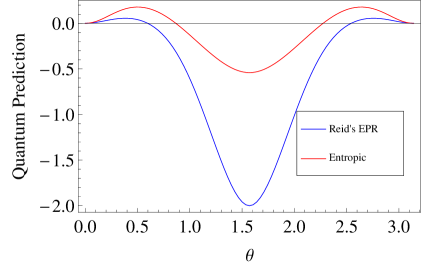
Figure 1: The quantum prediction of Reid’s EPR inequality and the entropic inequality by state (4). The critical values are $\theta_{c1}=0.5980$, $\theta_{c2}=0.8667$, $\theta_{c3}=2.2749$, $\theta_{c4}=2.5436$. When $\theta_{c1}<\theta<\theta_{c4}$, Reid’s EPR inequality is not violated; nor is the entropic inequality when $\theta_{c2}<\theta<\theta_{c3}$. Both criteria fail to detect EPR steering in the central region of $\theta$, but the entropic inequality is more efficient in the sense of broader violation region and larger maximal violation.

IV The Entropic inequality

In Ref. entropic the authors have developed an entropic inequality based on Heisenberg uncertainty principle in the form of entropy. They demonstrated the reason why the entropic inequality is more efficient than Reid’s EPR inequality, that is the latter focuses on up to second-order of the ovservables, while the former includes more. They also provide an example with a Gaussian-type state

$$\Phi_{n}(x_{1},x_{2})$$

$$\;\;=\mathcal{C}_{n}\mathcal{H}_{n}(\frac{x_{1}+x_{2}}{\sqrt{2}\sigma_{+}})e^{-(x_{1}+x_{2})^{2}/4\sigma_{+}^{2}}\times e^{-(x_{1}-x_{2})^{2}/4\sigma_{-}^{2}},$$

for which for up to $n\leq 15$ the entropic inequality is obviously more efficient than Reid’s EPR inequality to detect EPR steering for the whole range of parameters $\sigma_{\pm}$. Here $\mathcal{C}_{n}$ is normalization constant.

The entropic inequality reads

$$\mathcal{I}_{\rm ent}={\rm ln}(\pi e)-h(X_{2}|X_{1})-h(P_{2}|P_{1})\leq 0,$$ (17)

where average conditional entropy $h(X_{2}|X_{1})=\int dx_{1}\mathcal{P}(x_{1})h(X_{2}|x_{1})$. Here $h(X)$ is the Shannon entropy for coordinate, that is,

$$h(X)=-\int dx\mathcal{P}(x){\rm ln}\mathcal{P}(x),$$ (18)

and similarly for average conditional entropy $h(P)$ for momentum. Explicitly,

$$h(X_{2}|X_{1}) = -\int_{-\infty}^{+\infty}dx_{1}\int_{-\infty}^{+\infty}dx_{2}\mathcal{P}(x_{1},x_{2}){\rm ln}\frac{\mathcal{P}(x_{1},x_{2})}{\mathcal{P}(x_{1})}$$ (19)

$$= -\int_{-\infty}^{+\infty}dx_{1}\int_{-\infty}^{+\infty}dx_{2}\mathcal{P}(x_{1},x_{2}){\rm ln}\mathcal{P}(x_{1},x_{2})$$

$$+\int_{-\infty}^{+\infty}dx_{1}\mathcal{P}(x_{1}){\rm ln}{\mathcal{P}(x_{1})}.$$

Taking into account (III) (13) (III) and (16), the quantum prediction $\mathcal{I}_{ent}$ with respect to different $\theta$ is plot in Fig. 1 (see the red line). We find that when $\theta_{c2}<\theta<\theta_{c3}$, the entropic inequality is not violated. Similar to Reid’s EPR inequality, the entropic inequality (17) cannot always detect EPR steering of state (4), but its violation region of $\theta$ is broader and the maximal violation is larger than those of (6). This indeed reflects that the entropic inequality is more efficient than Reid’s EPR inequality.

For comparison, state (5) is considered and the quantum prediction $\mathcal{I}_{\rm Reid}$ and $\mathcal{I}_{\rm ent}$ are shown in Fig. 2. The entropic inequality again demonstrates its advantage on broader violation region than Reid’s EPR inequality. But for $0\leq\theta\leq\theta_{d1}$ and $\theta_{d4}\leq\theta\leq\pi$, EPR steering still cannot be detected.

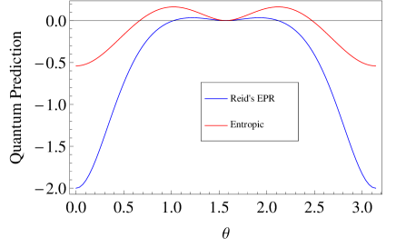
Figure 2: The quantum prediction of Reid’s EPR inequality and the entropic inequality by state (5). The critical values are $\theta_{d1}=0.6669$, $\theta_{d2}=1.0216$, $\theta_{d3}=2.1200$, $\theta_{d4}=2.4746$. Reid’s EPR inequality is violated when $\theta_{d2}<\theta<\theta_{d3}$, so is the entropic inequality when $\theta_{d1}<\theta<\theta_{d4}$, except $\theta=\pi/2$.

V Discussion

Let us discuss the Bell nonlocality of states (4) and (5). The CHSH CHSH inequality reads

$$I_{\rm CHSH}=Q_{11}+Q_{12}+Q_{21}-Q_{22}\leq 2,$$ (20)

where correlation function $Q_{ij}={\rm Tr}[\rho\vec{\sigma}\cdot\vec{a}_{i}\otimes\vec{\sigma}\cdot\vec{b}_{j}]$, $\vec{a}_{i}$ and $\vec{b}_{j}$ are three dimensional unit vectors, $\vec{\sigma}=(\sigma_{x},\sigma_{y},\sigma_{z})$ is pseudo-Pauli matrix vector ZBCHEN with

$$\sigma_{x} = \sum_{n=0}^{\infty}[|2n+1\rangle\langle 2n|+|2n\rangle\langle 2n+1|],$$

$$\sigma_{y} = \sum_{n=0}^{\infty}[i|2n+1\rangle\langle 2n|-i|2n\rangle\langle 2n+1|],$$

$$\sigma_{z} = \sum_{n=0}^{\infty}[|2n\rangle\langle 2n|-|2n+1\rangle\langle 2n+1|].$$ (21)

For the density function $\rho=|\Psi(x_{1},x_{2})|^{2}$ or $\rho=|\Psi^{\prime}(x_{1},x_{2})|^{2}$, by choosing some appropriate settings $\vec{a}_{i},\vec{b}_{j}$, we have the maximal quantum violation as

$$\mathcal{I}_{\rm CHSH}^{Q}=2\sqrt{1+\sin^{2}(2\theta)}\geq 2.$$ (22)

This indicates that the CV wavefunctions $\Psi(x_{1},x_{2}),\Psi^{\prime}(x_{1},x_{2})$ always have Bell nonlocality in the region $\theta\in(0,\pi)$ except $\theta=\pi/2$.

According to the hierarchy of nonlocal correlations, it implies that wavefunctions $\Psi(x_{1},x_{2}),\Psi^{\prime}(x_{1},x_{2})$ always have EPR steering in the region $\theta\in(0,\pi)$ except $\theta=\pi/2$, as they always have Bell nonlocality in the corresponding region. However Reid’s EPR inequality and the entropic inequality cannot detect all the EPR steering for states (4) and (5), this suggests that both criteria are not necessary and sufficient conditions to detect the EPR steering. The solution to this problem may deepen the understanding of nonlocal correlations and cause far-reaching effect on the classical-quantum correspondence as well.

ACKNOWLEDGEMENTS

J.L.C. is supported by National Basic Research Program (973 Program) of China under Grant No. 2012CB921900 and NSF of China (Grant Nos. 10975075 and 11175089). This work is also partly supported by National Research Foundation and Ministry of Education, Singapore (Grant No. WBS: R-710-000-008-271).

References

• (1) M. A. Nielsen and I. L. Chuang, Quantum Computation and Quantum Information (Cambridge University Press, Cambridge, England, 2000).
• (2) M. Horodeckia, P. Horodeckib, and R. Horodeckic, Phys. Lett. A 223, 1 (1996).
• (3) R. Horodecki, P. Horodecki, M. Horodecki, and K. Horodecki, Rev. Mod. Phys. 81, 865 (2009).
• (4) P. Horodecki, Phys. Lett. A 232, 333 (1997).
• (5) M. Horodecki, P. Horodecki, and R. Horodecki, Phys. Rev. Lett 80, 5239 (1998).
• (6) J. S. Bell, Physics (Long Island City, N.Y.) 1, 195 (1964).
• (7) J. Clauser, M. Horne, A. Shimony, and R. Holt, Phys. Rev. Lett. 23, 880 (1969).
• (8) N. D. Mermin, Phys. Rev. Lett. 65, 1838 (1990); M. Ardehali, Phys. Rev. A 46, 5375 (1992); A.V. Belinskii and D. N. Klyshko, Phys. Usp. 36, 653 (1993).
• (9) R. F. Werner and M.M. Wolf, Phys. Rev. A 64, 032112 (2001).
• (10) M. Żukowski and Č. Brukner, Phys. Rev. Lett. 88, 210401 (2002).
• (11) D. Collins, N. Gisin, N. Linden, S. Massar, and S. Popescu, Phys. Rev. Lett. 88, 040404 (2002).
• (12) Antonio Acín, Nicolas Gisin, and Benjamin Toner, Phys. Rev. A 73, 062105 (2006).
• (13) Tamás Vértesi and Károly F. Pál, Phys. Rev. A 84, 042122 (2011).
• (14) R. F. Werner, Phys. Rev. A 40, 4277 (1989).
• (15) H. M. Wiseman, S. J. Jones, and A. C. Doherty, Phys. Rev. Lett. 98, 140402 (2007).
• (16) S. J. Jones, H. M. Wiseman, and A. C. Doherty, Phys. Rev. A 76, 052116 (2007).
• (17) E. G. Cavalcanti, S. J. Jones, H. M. Wiseman, and M. D. Reid, Phys. Rev. A 80, 032112 (2009).
• (18) D. J. Saunders, S. J. Jones, H. M.Wiseman and G. J. Pryde, Nature Phys. 6, 845 (2009).
• (19) Q. Y. He, P. D. Drummond, and M. D. Reid, Phys. Rev. A 83, 032120 (2011).
• (20) A. Einstein, B. Podolsky, and N. Rosen, Phys. Rev. 47, 777 (1935).
• (21) E. G. Cavalcanti, Q. Y. He, M. D. Reid, H. M. Wiseman , Phys. Rev. A 84, 032115 (2011).
• (22) M. D. Reid, Phys. Rev. A 40, 913 (1989).
• (23) M. D. Reid, P. D. Drummond, W. P. Bowen, E. G. Cavalcanti, P. K. Lam, H. A. Bachor, U. L. Anderson, and G. Leuchs, Rev. Mod. Phys. 81, 1727 (2009).
• (24) Z. Y. Ou, S. F. Pereira, H. J. Kimble, and K. C. Peng, Phys. Rev. Lett. 68, 3663 (1992).
• (25) J. C. Howell, R. S. Bennink, S. J. Bentley, and R. W. Boyd, Phys. Rev. Lett. 92, 210403 (2004).
• (26) S. P. Walborn, A. Salles, R. M. Gomes, F. Toscano, and P. H. Souto Ribeiro, Phys. Rev. Lett. 106, 130402 (2011).
• (27) Z. B. Chen, J. W. Pan, G. Hou, and Y. D. Zhang, Phys. Rev. Lett. 88, 040406 (2002).