Production of a KK-graviton in association with a boson via gluon fusion at the LHC

Abstract:

We discuss the processes where a KK-graviton ($G$) of the extra-dimensional models is produced in association with a color singlet boson via gluon fusion at the LHC. In particular, we consider the processes $gg\to hG$, $\gamma G$, $ZG$. These processes occur at one-loop through box and triangle diagrams. The cross-section for the process $gg\to\gamma G$ vanishes at the one-loop level. It can be understood by introducing the charge conjugation transformations of the KK-graviton. The processes $gg\to hG$, $ZG$ can be observed at the LHC if the KK-graviton and the Higgs boson exist with appropriate properties.

1 Introduction

Various extra-dimensional extensions of the Standard Model (SM) [1, 2, 3, 4, 5] have attracted a lot of interest in the recent literature. In these models, the number of spacial dimensions is assumed to be more than $3$ with the extra dimensions being hidden (compactified). Apart from the compactification mechanism, different models differ on the size as well as the number of the extra dimensions. Although, depending on the model, the SM fields can either propagate in the bulk or live on a boundary of the bulk, gravity can freely propagate through the extra-dimensions. In the low energy 4-D picture gravity is treated as an effective theory with the graviton fields appearing as towers of KK-excitation modes (KK-gravitons).

The Large Hadron Collider (LHC) provides us with a unique opportunity to observe experimental signatures of these KK-gravitons. For possible signals, several people have studied different production processes of spin-2 KK-gravitons (referred to as graviton in the rest of the paper) in association with some vector boson in the LHC [6, 7, 8, 9]. Except for the case where the final state vector boson is a gluon, these papers consider only the $q\bar{q}$ initiated processes. Here our focus is on a different initial state – we discuss the two gluon initiated graviton production in association with a scalar/vector boson ($gg\rightarrow G\mathcal{B}$). Since gravitons couple with matter via energy-momentum tensor, only the $gg\rightarrow Gg$ process has a tree level contribution. For all the other bosons the corresponding process mediates via quark loops. We restrict ourselves to color singlet final states and consider the following processes – (i) $gg\rightarrow Gh$, (ii) $gg\rightarrow G\gamma$ and (iii) $gg\rightarrow GZ$.

At the LHC, the gluon flux dominates over the quark-flux. Hence, although loop mediated, gluon fusion contributions to the processes with the color singlet bosons need not be negligible. For the Higgs case, gluon fusion is the dominant channel in the LHC. The cross-sections for this process in two different extra-dimensional models like ADD [1] and RS1 [2] have been reported earlier [10]. In this paper we briefly describe the calculation and summarize the results. For the case of photon, however, gluon fusion gives zero contribution. This follows from the introduction of C-parity of the graviton. We present a small field theoretic proof of this argument. We present some results for the $Z$-boson case – the details of this calculation will be reported elsewhere [11].

2 Graviton with a Higgs Boson

As already mentioned, the gluon fusion mechanism ($gg\rightarrow hG$) is the dominant channel for the production of a Higgs boson in association with a graviton at the LHC [10]. Since both the final state particles are color singlet, diagrams containing three gluon vertices are absent because of the color conservation. The first non vanishing contribution to the $gg\rightarrow hG$ process comes from the diagrams containing a quark loop (at $\mathcal{O}(g^{2}_{s}\kappa y_{q})$). However, because of the presence of the Yukawa coupling ($y_{q}$) only the top-quark loop contributes significantly. There are six box diagrams and twelve triangle diagrams (see Figs. 1 – 1), of which only half are independent as they are related to the others by charge conjugation. Moreover the contribution from the triangle diagrams with a $hqqG$ vertex (Fig. 1) vanishes – this vertex is proportional to the metric, $\eta_{\mu\nu}$, which when contracted with the graviton polarization tensor gives zero.

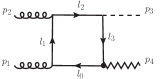
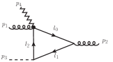
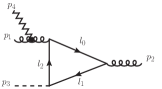
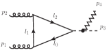
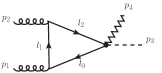
Figure 1: Different classes of diagrams for the process $gg\rightarrow hG$. The complete set of diagrams can be obtained by permuting the external particles. The zigzag lines denote the graviton and the dashed lines denote the Higgs.

2.1 Computation

Feynman rules for the vertices required to calculate these diagrams can be found in [12]. After computing the traces associated with the top-quark loops using FORM [13], the amplitude contains tensor loop integrals, the most complicated of which are the rank-4 tensor-box integral ($D^{\mu\nu\rho\sigma}$) among the the box integrals while rank-2 tensor-triangle integral ($C^{\mu\nu}$) among the triangle ones,

$$D^{\mu\nu\rho\sigma}=\int\frac{d^{n}l_{0}}{(2\pi)^{n}}\frac{l_{0}^{\mu}l_{0}^{\nu}l_{0}^{\rho}l_{0}^{\sigma}}{D_{0}D_{1}D_{2}D_{3}}\,,\quad C^{\mu\nu}=\int\frac{d^{n}l_{0}}{(2\pi)^{n}}\frac{l_{0}^{\mu}l_{0}^{\nu}}{D_{0}D_{1}D_{2}}\,,$$ (1)

where $D_{i}=l_{i}^{2}-m_{t}^{2}+i\varepsilon$ and $n=4-2\epsilon$ (see Figs. 1 - 1 for the definition of $l_{i}$’s). These tensor integrals were reduced into the standard scalar integrals – $A_{0}$, $B_{0}$, $C_{0}$ and $D_{0}$ using fortran routines [14] that follows the reduction scheme developed by Oldenborgh and Vermaseren [15]. The scalar integrals (with massive internal lines) were ultimately called from FF library [16]. Helicity basis for the polarization vectors were used to calculate the amplitude.

To compute the cross-section, numerical integrations were performed over the two body phase space, momentum fractions ($x_{1}/x_{2}$) of the initial state gluons and over the graviton mass parameter in the continuum approximation (for the ADD model [1, 12]). As a cautionary check, the following tests were made with the code.

1. UV Finiteness: The UV finiteness of the total amplitude were tested by varying the renormalization scale ($\mu_{\rm R}$) over ten orders of magnitude. The amplitude is independent of the actual value of $\mu_{\rm R}$. The triangle and box amplitudes are separately UV finite. Each triangle diagram is UV finite by itself.

2. Gauge Invariance: The amplitude was ensured to be gauge invariant with respect to both the gluons. This was done by replacing the polarization vector of either of the gluons by its momentum ($\varepsilon^{\mu}(p_{i})\rightarrow p^{\mu}_{i}$) which made the amplitude vanish. Some of the triangle diagrams are separately gauge invariant with respect to both the gluons. To ensure the correctness of their contribution towards the full amplitude, gauge invariance check with respect to the graviton polarization was also performed.

2.2 Results

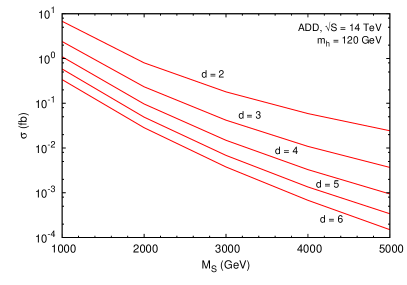
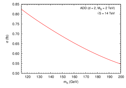
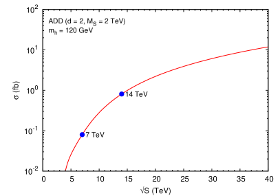
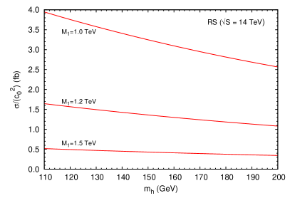
Figure 2: Process $gg\to Gh$: (a) Variation of the cross-section ($\sigma$) with the cutoff scale ($M_{\rm S}$) of the ADD model [1] for different numbers of extra dimensions, $d$. (b) Variation of $\sigma$ with mass of the Higgs, $m_{h}$. (c) Variation of $\sigma$ with $E_{cm}$. (d) The cross-section, $\sigma$ for the production of the first KK mode of the graviton with the Higgs scaled by the square of the dimensionless coupling parameter $c_{0}=k/{\bar{M}}_{\rm P}=\sqrt{8\pi}k/M_{\rm P}$ in the RS1 model [2]. Here $M_{1}$ denotes the mass of the first KK mode of the graviton.

In Figs. 2 – 2 we display the results for the KK-graviton production in association with a Higgs boson. Fig. 2 shows the dependence of the cross-section on the two parameters of the ADD model [1], i.e., the cut-off scale, $M_{\rm S}$ and the number of extra dimensions, $d$. Fig. 2 shows how the cross-section goes down (mainly because of phase space suppression) with increasing Higgs mass and Fig. 2 shows the dependence of $\sigma$ on the center of mass energy, $E_{cm}$. In Fig. 2 we show the cross-section in the RS1 model [2] scaled by the square of the dimensionless coupling parameter $c_{0}=k/{\bar{M}}_{\rm P}=\sqrt{8\pi}k/M_{\rm P}$. In general $c_{0}$ is assumed to be between 0.01 and 0.1. These plots were obtained using NLO CTEQ6M PDFs and applying the following cuts on the transverse momentum and rapidity of the Higgs: $p_{\rm T}^{h}>20$ GeV, $|\eta^{h}|<2.5$. In case of the ADD model, one extra cut was applied on the invariant mass of the outgoing particles: $M(hG)\leq M_{\rm S}$ (truncated scheme).

We found a large cancelation between the box-diagrams contribution and the triangle-diagrams contribution that reduces the amplitude by two-to-three orders of magnitude. This, in turn, reduces the cross-section to the order of 1 fb or smaller for most of the parameter ranges of the ADD model. Still, one could expect few hundred such events after the LHC achieves its design luminosity if $d\sim 2-3$ and $M_{\rm S}\sim 1-3$ TeV. This process can be observed at LHC with a few years of operation. However in the RS1 model, the cross-section becomes even smaller. For example for $c_{0}=0.075$, $M_{1}=1$ TeV and $m_{h}=120$ GeV the cross-section is only about 0.02 fb.

Finally, before we move on to the next section, one comment on the effect of the mass of top quark is in order. We find that the top quark does not decouple even as its mass, $m_{t}$ increases. In the beginning the cross-section increases because of the propagator enhancement. However, beyond $m_{t}\approx 400$ GeV, cross-section decreases and approaches a constant value beyond $m_{t}\gtrsim 2$ TeV. This behavior is similar to what has been seen in the case of $gg\rightarrow h$ production within the SM.

3 Graviton with a Photon

Photons do not have any charge (quantum number) and hence they are eigenstates of the Charge Conjugation (CC) operator $\mathcal{C}$. Invariance of the QED Lagrangian under CC implies,

$${\mathcal{C}}A_{\mu}{\mathcal{C}}^{\dagger}=\eta_{\gamma}A_{\mu}\,,\quad\eta_{\gamma}=-1\,,$$ (2)

i.e., photons have negative C-parity. As a result there is no process with only odd number of external photons in QED. This is known as the Furry’s Theorem [17, 18]. To construct a field theoretic proof of this theorem let us consider the photon $n$-point Green’s function,

$$\Gamma_{\mu_{1}\cdots\mu_{n}}=\frac{1}{\mathcal{N}}\left<0\left|{\sf T}\left[A_{\mu_{1}}(x_{1})A_{\mu_{2}}(x_{2})\cdots A_{\mu_{n}}(x_{n})\exp\left[i\int d^{4}x\,\mathcal{L}^{\rm QED}_{int}\right]\right]\right|0\right>\,,$$ (3)

where $\mathcal{N}$ is the normalization factor. As ${\mathcal{C}}^{\dagger}{\mathcal{C}}=1$,

$$\Gamma_{\mu_{1}\cdots\mu_{n}} = \frac{1}{\mathcal{N}}\left<0\left|{\sf T}\left[{\mathcal{C}}^{\dagger}{\mathcal{C}}A_{\mu_{1}}(x_{1}){\mathcal{C}}^{\dagger}{\mathcal{C}}\cdots{\mathcal{C}}^{\dagger}{\mathcal{C}}A_{\mu_{n}}(x_{n}){\mathcal{C}}^{\dagger}{\mathcal{C}}\exp\left[i\int d^{4}x\,\mathcal{L}^{\rm QED}_{int}\right]{\mathcal{C}}^{\dagger}{\mathcal{C}}\right]\right|0\right>$$ (4)

$$= (-1)^{n}\Gamma_{\mu_{1}\cdots\mu_{n}}\,,$$

where we have used Eq. 2 and the fact that both the free vacuum and QED interactions are invariant under CC. Hence for odd $n$, the Green’s function vanishes. This proof shows that this result is valid at all orders of perturbation theory as long as the interaction terms remain invariant under CC. Moreover insertion of any number of C-even boson fields would not affect the result.

3.1 C-parity of Gravitons

We introduce C-parity of gravitons to examine processes involving gravitons, photons and gluons. To determine the C-parity of the gravitons, let us consider the graviton-electron interaction [12],

$$2\kappa^{-1}\mathcal{L}_{e}^{\vec{n}}=-G_{\mu\nu}\bar{\psi}_{e}i\gamma^{\mu}\href{http://www-spires.slac.stanford.edu/spires/find/hep/www?j=PHRVA\%2C^\%2C\psi}{{\it Phys.\ Rev.\ }{\bf^} (\nu) \psi}_{e}-\frac{1}{2}\bar{\psi}_{e}i\gamma^{\mu}\left(\href{http://www-spires.slac.stanford.edu/spires/find/hep/www?j=PHRVA\%2C^\%2CG}{{\it Phys.\ Rev.\ }{\bf^} (\nu) G}_{\mu\nu}\right)\psi_{e}\,.$$ (5)

As gravity couples only to the energy-momentum tensor, it is natural to assume that the gravitational interaction with matter, in particular with electron, is invariant under CC. Using CC properties of the Dirac fields and gamma matrices, we can determine that gravitons have positive C-parity,

$${\mathcal{C}}G_{\mu\nu}{\mathcal{C}}^{\dagger}=\eta_{G}G_{\mu\nu}\,,\quad\eta_{G}=1\,.$$ (6)

Therefore as discussed above, any process with only odd number of external photons and any number of external gravitons vanishes to all orders of perturbation theory, as long as we include only CC invariant interactions.

3.2 Furry’s Theorem with Gravitons, Photons and Two Gluons

Gluons carry color charges and hence are not eigenstates of ${\mathcal{C}}$. One cannot expect Furry’s theorem to work for process with only external gluons and indeed three gluon vertex exists even at the tree level. However, since QCD interactions are invariant under CC one can derive a transformation rule for gluons [20],

$${\mathcal{C}}g^{a}_{\mu}(x){\mathcal{C}}^{\dagger} = -\left[\Lambda\right]^{ab}g^{b}_{\mu}(x)\,,$$ (7)

where $\Lambda$ is a diagonal matrix with $\Lambda^{2}=1$. It is defined as,

$$\left[\tau^{a}\right]^{\rm T}=\left[\Lambda\right]^{ab}\tau^{b}\,,$$ (8)

where $\tau^{a}$’s are the $SU(3)_{c}$ generators. The Green’s function for a process with only $n$ number of external photons, $m$ number of external gravitons and two external gluons,

$$\Gamma_{\{\mu_{i}\}\{\alpha_{j}\beta_{j}\}\nu_{1}\nu_{2}}=\frac{\delta^{ab}}{\mathcal{N}}\left<0\left|{\sf T}\left[A_{\mu_{1}}\cdots A_{\mu_{n}}G_{\alpha_{1}\beta_{1}}\cdots G_{\alpha_{m}\beta_{m}}g^{a}_{\nu_{1}}g^{b}_{\nu_{2}}\exp\left[i\int d^{4}x\,\mathcal{L}_{int}\right]\right]\right|0\right>\,,$$ (9)

where $\delta^{ab}$ appears because of the conservation of color. Just like before we can incert ${\mathcal{C}}^{\dagger}{\mathcal{C}}$’s to get

$$\Gamma_{\{\mu_{i}\}\{\alpha_{j}\beta_{j}\}\nu_{1}\nu_{2}}=(-1)^{n}\left(\Lambda\right)^{2}\Gamma_{\{\mu_{i}\}\{\alpha_{j}\beta_{j}\}\nu_{1}\nu_{2}}=(-1)^{n}\Gamma_{\{\mu_{i}\}\{\alpha_{j}\beta_{j}\}\nu_{1}\nu_{2}}\,,$$ (10)

if $\mathcal{L}_{int}$ is invariant under charge conjugation. We see that the proof still works if we replace any two photons by gluons, i.e., force the two gluons to go into a color singlet state. Hence two gluons can not fuse into odd number of photons (or any C-odd boson) and any number of gravitons or any other C-even boson. This is strictly true at one loop level. However as already mentioned this result is valid at all orders of perturbation theory as long as we don’t include weak corrections, i.e., the interaction terms remain invariant under CC.

4 Graviton with a $Z$-boson

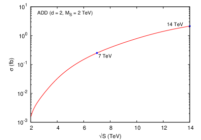
Figure 3: Variation of $\sigma$ with $E_{cm}$ for the process $gg\to GZ$.

The production of a graviton in association with a Z-boson can occur at the tree level. One loop QCD corrections to this process have also been computed [6, 7]. However, this radiative correction calculation did not include the the gluon fusion channel. Because of the large gluon flux at the LHC, this production can make sizable correction to the tree-level contribution. This calculation has recently been performed [11].

The diagrams that contribute to the process $gg\to ZG$ belong to the same classes of the triangle and box diagrams as for the process $gg\to hG$. Because of the Furry’s theorem only the axial coupling of the Z-boson contributes to the amplitude in this process. There is also an additional complication – although this process is UV finite, the triangle and box diagrams are linearly divergent. Moreover the coupling to axial gauge current leads to anomalies. Therefore, one has to be careful in carrying out the computation and checking the gauge invariance. The contribution of the individual flavor of quarks will give anomalous contribution, but this contribution must cancel when we include the full generation of quarks. One also has to treat $\gamma_{5}$ in $d$-dimensions more carefully and use proper prescription.

The computation was done for the ADD model. The details of the calculation can be found in [11]. In Fig. 3, we have plotted the cross-section of the process as a function of the center of mass energy for $d=2$ and $M_{\rm S}=2$ TeV. For this, the following kinematic cuts were applied:

$$P_{T}^{Z}>30\textrm{ GeV},\quad|\eta^{Z}|<2.5,\quad M(GZ)\leq M_{\rm S}\textrm{ (truncated scheme)}.$$

The factorization and the renormalization scales were chosen as $\mu_{f}=\mu_{R}=E_{T}^{Z}\left(=\sqrt{M_{Z}^{2}+(P_{T}^{Z})^{2}}\right)$ and, just like the Higgs case, NLO CTEQ6M PDFs were used. We note that at typical LHC energy, the cross-section is of the order of few fb which is much smaller than expected. The cross-section becomes small because of a two-orders of magnitude cancellation in the amplitude between the box-type and triangle-type diagrams. It is similar to the case of $gg\to hG$ process. Still one may expect few hundred of such events after a few years of LHC operation at 14 TeV CM energy. Unlike the Higgs boson case where we don’t find any decoupling of the heavy quark, the heavy quark in the loop does decouple as its mass goes to infinity for this process.

5 Conclusions

We have examined the processes $gg\to hG,\gamma G,ZG$ at the LHC. These processes, though leading order, occur at one loop. We have generalized the Furry’s theorem to processes containing arbitrary number of photons, gravitons, and up to two gluons. According to this generalization, any process with only two gluons, odd number of photons and any number of gravitons vanish at one-loop order. This remains true to any order if we don’t include CC-violating interactions, such as weak interaction. As a consequence, the process $gg\to\gamma G$ does not get contribution at the one-loop level. In the calculation for the processes $gg\to hG,ZG$, there is a cancellation of two orders of magnitude between the box and the triangle-classes of diagrams. This reduces the cross-sections to the order of 1 fb for these processes. Still, with few years of the operation of LHC at the center of mass energy of $14$ TeV, one may be able to observe these processes.

References

- [1] N. Arkani-Hamed, S. Dimopoulos and G. R. Dvali, Phys. Lett. B 429 (1998) 263.
- [2] L. Randall and R. Sundrum, Phys. Rev. Lett. 83 (1999) 3370.
- [3] L. Randall and R. Sundrum, Phys. Rev. Lett. 83 (1999) 4690.
- [4] I. Antoniadis, Phys. Lett. B 246 (1990) 377.
- [5] T. Appelquist, H. C. Cheng and B. A. Dobrescu, Phys. Rev. D 64 (2001) 035002.
- [6] M. C. Kumar, P. Mathews, V. Ravindran and S. Seth, J. Phys. G 38 (2011) 055001.
- [7] M. C. Kumar, P. Mathews, V. Ravindran and S. Seth, Nucl. Phys. B 847 (2011) 54.
- [8] S. Karg, M. Kramer, Q. Li and D. Zeppenfeld, Phys. Rev. D 81 (2010) 094036.
- [9] X. Gao, C. S. Li, J. Gao, J. Wang and R. J. Oakes, Phys. Rev. D 81 (2010) 036008.
- [10] A. Shivaji, S. Mitra and P. Agrawal, 1108.4561 [hep-ph].
- [11] A. Shivaji, V. Ravindran and P. Agrawal, in preparation.
- [12] T. Han, J. D. Lykken and R. J. Zhang, Phys. Rev. D 59 (1999) 105006.
- [13] J. A. M. Vermaseren, math-ph/0010025.
- [14] P. Agrawal and G. Ladinsky, Phys. Rev. D 63 (2001) 117504.
- [15] G. J. van Oldenborgh and J. A. M. Vermaseren, Z. Phys. C 46 (1990) 425.
- [16] G. J. van Oldenborgh, Comput. Phys. Commun. 66 (1991) 1.
- [17] W. H. Furry, Phys. Rev., 51 (1937) 125.
- [18] K. Nishijima, Prog. Theor. Phys., 6 (1951) 614.
- [19] C. N. Yang, Phys. Rev. 77 (1950) 242.
- [20] I. V. Tyutin and B. B. Lokhvitskii, Russian Physics Journal, 25 (1982) 346.