$z\rightarrow-z$ symmetry of spin-orbit coupling and weak localization in graphene

Abstract

We show that the influence of spin-orbit (SO) coupling on the weak localization effect for electrons in graphene depends on the lack or presence of $z\rightarrow-z$ symmetry in the system. While for $z\rightarrow-z$ asymmetric SO coupling, disordered graphene should display a weak anti-localization behavior at lowest temperature, $z\rightarrow-z$ symmetric coupling leads to an effective saturation of decoherence time which can be partially lifted by an in-plane magnetic field, thus, tending to restore the weak localization effect.

The effect of spin-orbit (SO) coupling in graphene represents an example of a stimulating theoretical study that remains difficult to detect experimentally. The form of intrinsic SO coupling in the graphene band structure, suggested by Kane and Mele kanemele05 , has fuelled the theory of $Z_{2}$ topological insulators, but its strength is too weak for detection by conventional spectroscopic methods kanemele05 ; dhh06 ; min06 ; yao07 ; dhh09 . Here, we show how the presence of SO coupling in disordered graphene could be manifested in quantum transport measurements. Specifically for graphene, the presence of SO coupling may not necessarily lead to anti-localization behavior known in semiconductors and metals LarkinWAL , and this reflects the presence or lack of $z\rightarrow-z$ symmetry in the source of SO coupling.

In general, weak localization is very sensitive to symmetry breaking in the electronic system or to scattering involving electron spin since it is formed by electrons propagating along long diffusive trajectories WL ; LarkinWAL ; AndoWL ; mor06 ; guinea06 ; WLmono ; WLreview ; tik08 ; koz11 ; lara11 ; imura09 . The typical behavior of electrons in metals with strong SO coupling results in a pronounced weak antilocalization effect manifested by positive magnetoresistance, in contrast to simple metals and semiconductors where the weak localization magnetoresistance caused by the interference correction to conductivity is negative. For graphene with broken $z\rightarrow-z$ symmetry, by a substrate or deposits, we find that, at the lowest temperatures, SO interaction leads to the conventional weak antilocalization. In contrast, for a $z\rightarrow-z$ symmetric system, SO coupling leads only to a saturation in the size of the weak localization correction rather than antilocalization, which can be taken for a saturation of $\tau_{\varphi}(T)$ as $T\rightarrow 0$. Then, we analyze the influence of an in-plane magnetic field on the interference correction to conductivity for both $z\rightarrow-z$ symmetric and antisymmetric SO coupling scenarios and find that it lifts the aforementioned saturation of $\tau_{\varphi}$.

The breaking of $z\rightarrow-z$ symmetry in pristine graphene is usually associated with the addition of a Bychkov-Rashba term ${\hat{h}}_{BR}$ kanemele05 ; rashba ; dhh06 ; min06 ; rasbagraphene ; imura09 ; dhh09 ; cn09 to the intrinsic SO coupling ${\hat{h}}_{KM}$ kanemele05 ; min06 ; yao07 ; imura09 in the graphene Hamiltonian:

$$\!\!\!\!\!\!\!\!\!\!\!\!\!\!\!\!\!\!\!\!\!\!\!\!\!\!\!{\hat{H}}\!=\!v\mbox{\boldmath$\Sigma$}\mathbf{p}+{\hat{h}}_{KM}+{\hat{h}}_{BR}+{\hat{U}}+{\hat{V}}_{\mathrm{sym}}+{\hat{V}}_{\mathrm{asy}}+\mu_{B}\mathbf{s}\mathbf{B}_{\parallel},$$

$${\hat{h}}_{KM} = \lambda\Sigma_{z}s_{z},\qquad{\hat{h}}_{BR}=\mu\left(\Sigma_{x}s_{y}-\Sigma_{y}s_{x}\right).$$ (1)

The last term in ${\hat{H}}$ accounts for Zeeman splitting due to in-plane magnetic field $\mathbf{B}_{\parallel}={\vec{\ell}}B_{\parallel}$, and the terms

$${\hat{U}} = u_{0}\,\mathrm{\hat{I}}+\sum_{a,l=x,y,z}\!u_{a,l}\,\Sigma_{a}\Lambda_{l},$$ (2)

$${\hat{V}}_{\mathrm{sym}} = s_{z}\Big{[}\sum_{a=x,y,z}\!\alpha_{a,z}\Sigma_{a}+\sum_{l=x,y,z}\!\beta_{l,z}\Lambda_{l}\Big{]},$$ (3)

$${\hat{V}}_{\mathrm{asy}} = \sum_{j=x,y}s_{j}\Big{[}\sum_{a=x,y,z}\alpha_{a,j}\Sigma_{a}+\sum_{l=x,y,z}\beta_{l,j}\Lambda_{l}\Big{]},$$ (4)

describe three types of disorder on the honeycomb lattice: spin-independent perturbations, SO coupling with $z\rightarrow-z$ symmetric perturbations, and $z\rightarrow-z$ asymmetric perturbations, respectively. Here, we use a symmetry-based approach to determine how electronic spin may be combined with lattice and valley degrees of freedom. We focus on the region near the Fermi level which lies in the vicinity of two inequivalent corners of the Brillouin zone, known as valleys, with wave vectors $\mathbf{K}_{\pm}=\pm(4\pi/3a,0)$ where $a$ is the lattice constant, and the momentum measured from the center of a valley is $\mathbf{p}=\hbar\mathbf{k}-\hbar\mathbf{K}_{\pm}$. The Hamiltonian (1) operates in a space of eight-component Bloch functions $\Phi=$[$\phi_{\mathbf{K}_{+},A,\uparrow}$, $\phi_{\mathbf{K}_{+},B,\uparrow}$, $\phi_{\mathbf{K}_{-},B,\uparrow}$, $\phi_{\mathbf{K}_{-},A,\uparrow}$, $\phi_{\mathbf{K}_{+},A,\downarrow}$, $\phi_{\mathbf{K}_{+},B,\downarrow}$, $\phi_{\mathbf{K}_{-},B,\downarrow}$, $\phi_{\mathbf{K}_{-},A,\downarrow}$ consisting of two valleys $\mathbf{K}_{+}$/$\mathbf{K}_{-}$, two lattice sites $A$/$B$, and two spin components $\uparrow$/$\downarrow$. We use three sets of Pauli matrices WLmono ; WLreview to describe spin $\vec{s}=(s_{x},s_{y},s_{z})$, sublattice ‘isospin’ $\vec{\Sigma}=(\Sigma_{x},\Sigma_{y},\Sigma_{z})$ and valley ‘pseudospin’ $\vec{\Lambda}=(\Lambda_{x},\Lambda_{y},\Lambda_{z})$ matrices . The matrices $\vec{s},\vec{\Sigma},\vec{\Lambda}$ all change sign upon time inversion so that their products are time-inversion symmetric and $\Sigma_{a}s_{j}$, $s_{j}\Lambda_{l}$ may be used as a basis for a phenomenological description of static disorder leading to SO scattering.

Table 1: Irreducible representations of the planar group $C_{6v}^{\prime\prime}$ groups , as provided by matrices $\Sigma_{a}$, $\Lambda_{l}$, and $s_{j}$. Representations $A_{1}$, $A_{2}$, $B_{1}$, $B_{2}$, $E_{1}$, $E_{2}$ are part of the point group of two-dimensional graphene $C_{6v}$, representations $E_{1}^{\prime}$, $E_{2}^{\prime}$, $G^{\prime}$ incorporate primitive translations.

Irr. Rep.	$z\rightarrow-z$ symmetric	$z\rightarrow-z$ asymmetric
$A_{1}$	$\hat{I}$, $\Sigma_{z}s_{z}$	$\Sigma_{x}s_{y}-\Sigma_{y}s_{x}$
$A_{2}$	$\Sigma_{z}$, $s_{z}$	$\Sigma_{x}s_{x}+\Sigma_{y}s_{y}$
$B_{1}$	$\Lambda_{z}$
$B_{2}$	$\Sigma_{z}\Lambda_{z}$, $\Lambda_{z}s_{z}$
$E_{1}$	$\left(\!\begin{array}[]{c}\Sigma_{x}\\ \Sigma_{y}\\ \end{array}\!\!\right)$ ​​, ​​​ $\left(\!\begin{array}[]{c}\Sigma_{x}s_{z}\\ \Sigma_{y}s_{z}\\ \end{array}\!\!\right)$	$\left(\!\begin{array}[]{c}s_{x}\\ s_{y}\\ \end{array}\!\!\right)$ ​, ​​ $\left(\!\begin{array}[]{c}\Sigma_{z}s_{x}\\ \Sigma_{z}s_{y}\\ \end{array}\!\!\right)$
$E_{2}$	$\left(\!\begin{array}[]{c}\Lambda_{z}\Sigma_{x}\\ \Lambda_{z}\Sigma_{y}\\ \end{array}\!\!\right)$	$\left(\!\begin{array}[]{c}\Sigma_{x}s_{y}+\Sigma_{y}s_{x}\\ \Sigma_{x}s_{x}-\Sigma_{y}s_{y}\\ \end{array}\!\!\right)$ ​​,​​ $\left(\!\begin{array}[]{c}\Lambda_{z}s_{x}\\ \Lambda_{z}s_{y}\\ \end{array}\!\!\right)$
$E_{1}^{\prime}$	$\left(\!\begin{array}[]{c}\Lambda_{x}\Sigma_{z}\\ \Lambda_{y}\Sigma_{z}\\ \end{array}\!\!\right)$ ​​,​​ $\left(\!\begin{array}[]{c}\Lambda_{x}s_{z}\\ \Lambda_{y}s_{z}\\ \end{array}\!\!\right)$
$E_{2}^{\prime}$	$\left(\!\begin{array}[]{c}\Lambda_{x}\\ \Lambda_{y}\\ \end{array}\!\!\right)$
$G^{\prime}$	$\left(\begin{array}[]{c}\Lambda_{x}\Sigma_{x}\\ \Lambda_{x}\Sigma_{y}\\ \Lambda_{y}\Sigma_{x}\\ \Lambda_{y}\Sigma_{y}\\ \end{array}\right)$	$\left(\begin{array}[]{c}\Lambda_{x}s_{x}\\ \Lambda_{x}s_{y}\\ \Lambda_{y}s_{x}\\ \Lambda_{y}s_{y}\\ \end{array}\right)$

The results of this symmetry-based approach are summarized in Table 1 which shows how $\vec{s},\vec{\Sigma},\vec{\Lambda}$ may be combined to form irreducible representations of the planar group $C_{6v}^{\prime\prime}$ groups which combines the point group $C_{6v}$ of strictly two-dimensional graphene with primitive translations, as appropriate for the description of two valleys $\mathbf{K}_{\pm}$. Matrices $\vec{\Sigma}$ and $\vec{\Lambda}$ are confined to the two-dimensional plane of graphene and their behavior under symmetry operations is impervious to the third spatial dimension. Thus, they are invariant under mirror reflection in the graphene plane so that, in the absence of spin, they only appear in the representations that are $z\rightarrow-z$ symmetric. The presence of spin, however, introduces a pseudovector that lies in three-dimensional space: $s_{z}$ is even under $z\rightarrow-z$ reflection, but in-plane components $s_{x},s_{y}$ are odd. Thus, SO terms containing $s_{z}$ appear in $z\rightarrow-z$ symmetric representations, terms containing $s_{x},s_{y}$ appear in $z\rightarrow-z$ asymmetric representations.

In Table 1, $\Sigma_{z}s_{z}$ is an invariant of the point group of graphene representing intrinsic Kane-Mele SO coupling ${\hat{h}}_{KM}$ kanemele05 ; min06 ; yao07 ; imura09 , and $\Sigma_{x}s_{x}-\Sigma_{y}s_{y}$ describes the Bychkov-Rashba term ${\hat{h}}_{BR}$ kanemele05 ; rashba ; dhh06 ; min06 ; rasbagraphene ; imura09 ; dhh09 ; cn09 which assumes the existence of a transverse field $\vec{\ell}_{z}$ breaking $z\rightarrow-z$ symmetry. The entries in Table 1 take into account possible SO scattering mechanisms due to defects in graphene: ${\hat{V}}_{\mathrm{sym}}$ includes terms proportional to $s_{z}$, and ${\hat{V}}_{\mathrm{asy}}$ includes $s_{x},s_{y}$. The term ${\hat{U}}$, Eq. (2), describes disorder decoupled from the spin degree of freedom: $u_{0}(\mathbf{r})\,\mathrm{\hat{I}}$ describing the influence of remote charges, $u_{z,z}(\mathbf{r})\Sigma_{z}\Lambda_{z}$ describing different on-site energies of the $A$/$B$ sublattices, and $u_{x,z}(\mathbf{r})\Sigma_{x}\Lambda_{z}$, $u_{y,z}(\mathbf{r})\Sigma_{y}\Lambda_{z}$ accounting for fluctuations of $A$/$B$ hopping. The other terms in ${\hat{U}}$, $u_{a,x}(\mathbf{r})\Sigma_{a}\Lambda_{x}$ and $u_{a,y}(\mathbf{r})\Sigma_{a}\Lambda_{y}$ for $a=x,y,z$, generate intervalley scattering. We assume that different types of disorder in the Hamiltonian are uncorrelated and $x$-$y$ isotropic:

$$\langle u_{a,l}\left(\mathbf{r}\right)u_{a^{\prime},l^{\prime}}\left(\mathbf{r^{\prime}}\right)\rangle = u_{a,l}^{2}\delta_{aa^{\prime}}\delta_{ll^{\prime}}\delta\left(\mathbf{r}-\mathbf{r^{\prime}}\right),$$

$$\langle\alpha_{a,j}\left(\mathbf{r}\right)\alpha_{a^{\prime},j^{\prime}}\left(\mathbf{r^{\prime}}\right)\rangle = \alpha_{a,j}^{2}\delta_{aa^{\prime}}\delta_{jj^{\prime}}\delta\left(\mathbf{r}-\mathbf{r^{\prime}}\right),$$

$$\langle\beta_{l,j}\left(\mathbf{r}\right)\beta_{l^{\prime},j^{\prime}}\left(\mathbf{r^{\prime}}\right)\rangle = \beta_{l,j}^{2}\delta_{ll^{\prime}}\delta_{jj^{\prime}}\delta\left(\mathbf{r}-\mathbf{r^{\prime}}\right).$$

Table 2: Scattering rates, due to symmetry-breaking terms in the Hamiltonian Eq. (1), that produce relaxation gaps $\Gamma_{j}^{l}$ in the otherwise gapless Cooperons ${C}_{j}^{l}$ where $j$ refers to spin, $l$ to valley. The relaxation rate of the intervalley Cooperons $\tau_{\ast}^{-1}$ and the intervalley rate $\tau_{iv}^{-1}$ result from spin-independent disorder, intrinsic $\tau_{KM}^{-1}$ and Bychkov-Rashba $\tau_{BR}^{-1}$ rates arise from coupling of spin and lattice, rates $\tau_{zv,\mathrm{e}}^{-1}$, $\tau_{zv,\mathrm{o}}^{-1}$, $\tau_{iv,\mathrm{e}}^{-1}$, $\tau_{iv,\mathrm{o}}^{-1}$ account for coupling of valley and spin degrees of freedom.

relaxation gaps

relaxation rates

$\Gamma_{0}^{0}=0$ $\Gamma_{0}^{x}=\Gamma_{0}^{y}=\tau_{\ast}^{-1}+2\tau_{zv,\mathrm{e}}^{-1}+4\tau_{zv,\mathrm{o}}^{-1}+2\tau_{iv,\mathrm{e}}^{-1}+4\tau_{iv,\mathrm{o}}^{-1}$ $\Gamma_{0}^{z}=2\tau_{iv}^{-1}+4\tau_{iv,\mathrm{e}}^{-1}+8\tau_{iv,\mathrm{o}}^{-1}$ $\Gamma_{x}^{0}=\Gamma_{y}^{0}=\tau_{BR}^{-1}+\tau_{KM}^{-1}+2\tau_{zv,\mathrm{e}}^{-1}+2\tau_{zv,\mathrm{o}}^{-1}+4\tau_{iv,\mathrm{e}}^{-1}+4\tau_{iv,\mathrm{o}}^{-1}$ $\Gamma_{x}^{x}=\Gamma_{x}^{y}=\Gamma_{y}^{x}=\Gamma_{y}^{y}=$ $\qquad\tau_{\ast}^{-1}+\tau_{BR}^{-1}+\tau_{KM}^{-1}+2\tau_{zv,\mathrm{o}}^{-1}+2\tau_{iv,\mathrm{e}}^{-1}+4\tau_{iv,\mathrm{o}}^{-1}$ $\Gamma_{x}^{z}=\Gamma_{y}^{z}=2\tau_{iv}^{-1}+\tau_{BR}^{-1}+\tau_{KM}^{-1}+2\tau_{zv,\mathrm{e}}^{-1}+2\tau_{zv,\mathrm{o}}^{-1}+4\tau_{iv,\mathrm{o}}^{-1}$ $\Gamma_{z}^{0}=2\tau_{BR}^{-1}+4\tau_{zv,\mathrm{o}}^{-1}+8\tau_{iv,\mathrm{o}}^{-1}$ $\Gamma_{z}^{x}=\Gamma_{z}^{y}=\tau_{\ast}^{-1}+2\tau_{BR}^{-1}+2\tau_{zv,\mathrm{e}}^{-1}+2\tau_{iv,\mathrm{e}}^{-1}+4\tau_{iv,\mathrm{o}}^{-1}$ $\Gamma_{z}^{z}=2\tau_{iv}^{-1}+2\tau_{BR}^{-1}+4\tau_{zv,\mathrm{o}}^{-1}+4\tau_{iv,\mathrm{e}}^{-1}$

$\tau_{\ast}^{-1}={\tau}_{z}^{-1}+\tau_{iv}^{-1}$ $\tau_{iv}^{-1}=\pi\gamma\left(u_{x,x}^{2}+u_{x,y}^{2}+u_{y,x}^{2}+u_{y,y}^{2}+u_{z,x}^{2}+u_{z,y}^{2}\right)/\hbar$ ${\tau}_{z}^{-1}=2\pi\gamma\left(u_{x,z}^{2}+u_{y,z}^{2}+u_{z,z}^{2}\right)/\hbar$ $\tau_{KM}^{-1}=\lambda^{2}/(\epsilon_{F}^{2}\tau_{0})+2\pi\gamma\left(\alpha_{x,z}^{2}+\alpha_{y,z}^{2}+\alpha_{z,z}^{2}\right)/\hbar$ $\tau_{BR}^{-1}=2\tau_{0}\mu^{2}/\hbar^{2}+\pi\gamma\left(\alpha_{x,x}^{2}+\alpha_{x,y}^{2}+\alpha_{y,x}^{2}+\alpha_{y,y}^{2}+\alpha_{z,x}^{2}+\alpha_{z,y}^{2}\right)/\hbar$ $\tau_{zv,\mathrm{e}}^{-1}=\pi\gamma\beta_{z,z}^{2}/\hbar$ $\tau_{iv,\mathrm{e}}^{-1}=\pi\gamma\beta_{x,z}^{2}/\hbar=\pi\gamma\beta_{y,z}^{2}/\hbar$ $\tau_{zv,\mathrm{o}}^{-1}=\pi\gamma\beta_{z,x}^{2}/\hbar=\pi\gamma\beta_{z,y}^{2}/\hbar$ $\tau_{iv,\mathrm{o}}^{-1}=\pi\gamma\beta_{x,x}^{2}/\hbar=\pi\gamma\beta_{x,y}^{2}/\hbar=\pi\gamma\beta_{y,x}^{2}/\hbar=\pi\gamma\beta_{y,y}^{2}/\hbar$ $\gamma=p_{F}/(2\pi\hbar^{2}v)$

In the following study, we employ the standard diagrammatic technique for disordered systems WL ; LarkinWAL to calculate the weak localization correction $\delta\sigma$ to the conductivity. We assume that the Dirac-like Hamiltonian $v\mbox{\boldmath$\Sigma$}.\mathbf{p}$ dominates the electronic behavior and that diagonal disorder, $\mathrm{\hat{I}}u_{0}(\mathbf{r})$ in Eq. (2), determines the elastic scattering rate, $\tau^{-1}\approx\tau_{0}^{-1}=\pi\gamma u^{2}/\hbar$, where $\gamma=p_{F}/(2\pi\hbar^{2}v)$ is the density of states per spin, per valley WLmono ; WLreview . The current operator corresponding to the Dirac-like Hamiltonian is momentum independent so that the current vertex entering the Drude conductivity is renormalized by vertex corrections. Then, the Drude conductivity is equal to $\sigma=4e^{2}\gamma D$ where the diffusion coefficient is $D=v^{2}\tau_{tr}/2$ and the transport time is twice the scattering time, $\tau_{tr}=2\tau_{0}$ AndoWL .

The weak localization correction $\delta\sigma$ may be written in terms of disorder-averaged two-particle correlation functions known as Cooperon propagators $C_{s}^{l}$ where index $l$ refers to pseudospin (related to $\vec{\Lambda}$ describing valley degrees of freedom), and $s$ refers to spin (related to $\vec{s}$). All the Cooperons that we consider are singlets with respect to sublattice isospin $\vec{\Sigma}$ because all isospin-triplet modes have relaxation gaps $\sim 1/\tau_{0}$ WLmono ; WLreview . Then, $\delta\sigma$ may be written in terms of a summation with respect to sixteen Cooperons consisting of combinations of spin and pseudospin singlet and triplets:

$$\delta\sigma=\frac{e^{2}D}{\pi\hbar}\sum_{s,l=0,x,y,z}c_{s}c_{l}\,{C}_{s}^{l}\left(\mathbf{r^{\prime}=\mathbf{r}}\right)\,,$$ (5)

$$\left[\!D\!\left(\!i\mathbf{\nabla}+\frac{2e\mathbf{A}}{c\hbar}\!\right)^{2}\!\!\!\!+\Gamma_{s}^{l}+\tau_{\varphi}^{-1}-i\omega\right]\!\!C_{s}^{l}\!\left(\mathbf{r},\mathbf{r^{\prime}}\right)=\delta\!\left(\mathbf{r}-\mathbf{r^{\prime}}\right).$$

Here, the factors $c_{0}=1$, $c_{x}=c_{y}=c_{z}=-1$ take into account the fact that singlet and triplet Cooperons (of both spin and pseudospin) appear with opposite signs, and $\mathbf{A}$ is the vector potential of homogeneous external magnetic field, $\mathbf{B}=\mathrm{rot}\mathbf{A}$ ($B_{z}=\partial_{x}A_{y}-\partial_{y}A_{x}$).

Inelastic dephasing is taken into account in Eq. (5) by $\tau_{\varphi}^{-1}$ and, in general, symmetry-breaking perturbations [such as those contained in the Hamiltonian Eq. (1)], contribute relaxation gaps $\Gamma_{s}^{l}$ to the otherwise gapless Cooperons ${C}_{s}^{l}$, as quantified in terms of relaxation rates summarized in Table 2. Then, the zero-field temperature-dependent correction, $\delta\rho\left(0\right)$, to the sheet resistance, where $\delta\rho\left(0\right)/\rho^{2}\equiv-\delta\sigma$, may be written as

$$\delta\rho\left(0\right) = -\frac{e^{2}\rho^{2}D}{\pi\hbar}\!\!\!\sum_{s,l=0,x,y,z}\!\!\!c_{s}c_{l}\!\int_{0}^{(D\tau)^{-1/2}}\!\!\!\frac{q\,dq}{2\pi}C_{s}^{l}(q),$$ (6)

$$= -\frac{e^{2}\rho^{2}}{2\pi h}\sum_{s,l=0,x,y,z}c_{s}c_{l}\,\ln\left(\frac{\tau^{-1}}{\tau_{\varphi}^{-1}+\Gamma_{s}^{l}}\right),$$ (7)

and the magnetoresistance, $\Delta\rho(B_{z})=\delta\rho\left(B_{z}\right)-\delta\rho\left(0\right)$, as

$$\delta\rho\left(B_{z}\right) = -\frac{e^{2}\rho^{2}D}{\pi\hbar}\!\!\!\sum_{s,l=0,x,y,z}\!\!\!c_{s}c_{l}\,\frac{eB_{z}}{\pi\hbar}\sum_{n=0}^{\tau_{B}/\tau}C_{s}^{l}(q_{n}),$$ (8)

$$\Delta\rho\left(B_{z}\right) = \frac{e^{2}\rho^{2}}{2\pi h}\sum_{s,l=0,x,y,z}c_{s}c_{l}\,F\!\left(\frac{B_{z}}{{\cal B}_{\varphi}+{\cal B}_{s}^{l}}\right),$$ (9)

$${\cal B}_{\varphi} = \frac{\hbar c}{4De}\tau_{\varphi}^{-1}\,,\qquad{\cal B}_{s}^{l}=\frac{\hbar c}{4De}\Gamma_{s}^{l}\,,$$

$$F\!\left(z\right) = \ln z+\psi\left(\frac{1}{2}+\frac{1}{z}\right)\,,$$

where $\psi$ is the digamma function. In Eq. (8) the influence of an external field $B_{z}$ is taken into account through discrete values $q_{n}^{2}=(n+1/2)/(D\tau_{B})$ where $\tau_{B}=\hbar/(4DeB_{z})$. Used in conjunction with the Cooperon gaps $\Gamma_{s}^{l}$ listed in Table 2, Eqs. (6-9) provide a general description of the weak-localization correction and corresponding low-field magnetoresistance in the presence of SO coupling in graphene, parameterized by six SO scattering rates $\tau_{KM}^{-1}$, $\tau_{BR}^{-1}$, $\tau_{zv,\mathrm{e}}^{-1}$, $\tau_{iv,\mathrm{e}}^{-1}$, $\tau_{zv,\mathrm{o}}^{-1}$, $\tau_{iv,\mathrm{o}}^{-1}$.

In order to analyze the influence of SO coupling in a realistic experimental situation tik08 ; koz11 ; lara11 , we consider - in the rest of this paper - the spin-independent intervalley scattering rate $\tau_{iv}^{-1}$ to exceed the decoherence rate $\tau_{\varphi}^{-1}$ and the rates due to SO coupling. This means that $\{\Gamma_{j}^{x},\Gamma_{j}^{y},\Gamma_{j}^{z}\}\gg\Gamma_{j}^{0}$ and, thus, the valley-triplet Cooperons in Eqs. (7-9) may be neglected. Then, the six SO rates may be combined into just two relevant combinations: a rate $\tau_{\mathrm{sym}}^{-1}$ due to $z\rightarrow-z$ symmetric SO coupling (terms ${\hat{V}}_{\mathrm{sym}}$ and ${\hat{h}}_{KM}$) and a rate $\tau_{\mathrm{asy}}^{-1}$ due to $z\rightarrow-z$ asymmetric coupling (${\hat{V}}_{\mathrm{asy}}$ and ${\hat{h}}_{BR}$):

$$\tau_{\mathrm{sym}}^{-1} = \tau_{KM}^{-1}+2\tau_{zv,\mathrm{e}}^{-1}+4\tau_{iv,\mathrm{e}}^{-1},$$ (10)

$$\tau_{\mathrm{asy}}^{-1} = \tau_{BR}^{-1}+2\tau_{zv,\mathrm{o}}^{-1}+4\tau_{iv,\mathrm{o}}^{-1}.$$ (11)

Here, $\tau_{BR}^{-1}$ accounts for the Dyakonov-Perel dpspin spin relaxation contribution, and the other terms for Elliott-Yafet eyspin spin relaxation.

The application of an in-plane magnetic field produces an interplay between SO coupling and Zeeman splitting, as in semiconductor quantum dots aleiner01 ; zumbuhl02 . In-plane magnetic field ${\vec{\ell}}B_{\parallel}$ introduces an additional term in the Hamiltonian $\delta{\hat{H}}=(\hbar\omega/2){\vec{\ell}}{\vec{s}}$ where $\omega=2\mu_{B}B_{\parallel}/\hbar$, $\epsilon_{z}=\hbar\omega$ is the Zeeman energy and ${\vec{\ell}}=(\ell_{x},\ell_{y},0)$, $|{\vec{\ell}}|=1$. This couples the spin-singlet $C_{0}^{0}$ to the triplets $C_{x}^{0}$ and $C_{y}^{0}$. The spin part of the matrix equation for the valley singlet Cooperons $(C_{0}^{0},C_{x}^{0},C_{y}^{0},C_{z}^{0})\equiv\mathbf{C}^{0}$ has the form

$$\left(\begin{array}[]{cccc}\Pi&-i\omega\ell_{x}&-i\omega\ell_{y}&0\\ -i\omega\ell_{x}&\Pi+\tau_{\mathrm{so}}^{-1}&0&0\\ -i\omega\ell_{y}&0&\Pi+\tau_{\mathrm{so}}^{-1}&0\\ 0&0&0&\Pi+2\tau_{\mathrm{asy}}^{-1}\end{array}\right)\mathbf{C}^{0}=1,$$

$$\Pi=D\left(i\mathbf{\nabla}+2e\mathbf{A}/c\hbar\right)^{2}+\tau_{\varphi}^{-1},$$

$$\!\!\!\!\!\!\!\!\!\!\!\!\!\!\!\!\!\!\!\!\!\!\!\!\!\!\!\!\!\!\!\!\!\!\!\!\tau_{\mathrm{so}}^{-1}=\tau_{\mathrm{sym}}^{-1}+\tau_{\mathrm{asy}}^{-1}.$$

After matrix inversion,

$$C_{0}^{0}\! = \!\frac{\Pi+\tau_{\mathrm{so}}^{-1}}{\Pi(\Pi+\tau_{\mathrm{so}}^{-1})+\omega^{2}}\xrightarrow[\epsilon_{z}\to\infty]{}0,$$

$$C_{x/y}^{0} = \frac{\Pi(\Pi+\tau_{\mathrm{so}}^{-1})+\omega^{2}(1-\ell_{x/y}^{2})}{(\Pi+\tau_{\mathrm{so}}^{-1})[\Pi(\Pi+\tau_{\mathrm{so}}^{-1})+\omega^{2}]}\xrightarrow[\epsilon_{z}\to\infty]{}\frac{1-\ell_{x/y}^{2}}{\Pi+\tau_{\mathrm{so}}^{-1}},$$

$$C_{z}^{0}\! = \!\frac{1}{\Pi+2\tau_{\mathrm{asy}}^{-1}}\xrightarrow[\epsilon_{z}\to\infty]{}\frac{1}{\Pi+2\tau_{\mathrm{asy}}^{-1}},$$

where the limit $\epsilon_{z}\to\infty$ of large Zeeman energy essentially means that $\epsilon_{z}\gg\hbar\tau_{\mathrm{so}}^{-1}$.

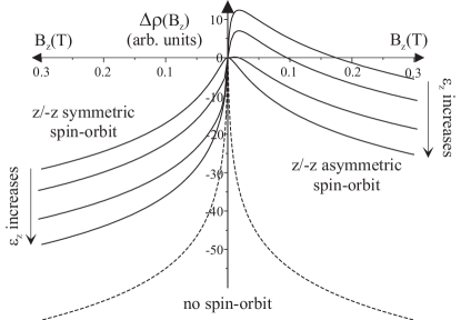
Figure 1: The low-field magnetoresistivity in the presence of $z\rightarrow-z$ symmetric (left) or asymmetric (right) SO scattering, as compared to the absence of SO scattering (lower dashed curves). Solid curves show the influence of SO scattering, $\tau_{\mathrm{sym}}^{-1}=25\tau_{\varphi}^{-1}$ and $\tau_{\mathrm{asy}}^{-1}=25\tau_{\varphi}^{-1}$, respectively, with Zeeman energy $\epsilon_{z}=0$ (top) to $\epsilon_{z}\gg\tau_{\mathrm{so}}^{-1}$ (bottom).

In the absence of in-plane field, $\epsilon_{z}=0$, the low-field magnetoresistance Eqs. (8,9) is given by

$$\!\!\!\!\!\!\!\!\!\Delta\rho\!=\!\frac{e^{2}\rho^{2}}{2\pi h}\!\!\left[F\!\!\left(\!\frac{B_{z}}{{\cal B}_{\varphi}}\!\right)\!-F\!\!\left(\!\frac{B_{z}}{{\cal B}_{\varphi}+{\cal B}_{\mathrm{asy}}}\!\right)\!-2F\!\!\left(\!\frac{B_{z}}{{\cal B}_{\varphi}+{\cal B}_{\mathrm{so}}}\!\right)\!\right]\!\!,$$

$${\cal B}_{\mathrm{asy}}=\frac{\hbar c}{2De}\tau_{\mathrm{asy}}^{-1},\qquad{\cal B}_{\mathrm{so}}=\frac{\hbar c}{4De}\tau_{\mathrm{so}}^{-1}.$$ (12)

In the absence of SO coupling, ${\cal B}_{\mathrm{so}}={\cal B}_{\mathrm{asy}}=0$, Eq. (12) would describe negative magnetoresistance corresponding to weak localization WLmono ; WLreview (lower dashed curves in Fig. 1). In the presence of $z\rightarrow-z$ symmetric SO coupling only, ${\cal B}_{\mathrm{asy}}=0$, the contribution of the third term in Eq. (12) is diminished, and the first and second terms cancel each other, leading to a suppression of magnetoresistance for $B_{z}\lesssim{\cal B}_{\mathrm{so}}$ (upper solid curve on the left of Fig. 1) which mimicks the effect of a saturated value of $\tau_{\varphi}^{-1}$: $\tau_{\varphi}^{-1}\rightarrow\tau_{\varphi}^{-1}+\tau_{\mathrm{sym}}^{-1}$. When $z\rightarrow-z$ symmetry is broken, ${\cal B}_{\mathrm{asy}}\neq 0$ and ${\cal B}_{\mathrm{so}}\neq 0$, there is relaxation of all spin-triplets, and the second and third terms in Eq. (12) are suppressed, leaving the first (singlet) term to determine anti-localization behavior at $T\to 0$ with positive magnetoresistance at low fields $B_{z}\lesssim{\cal B}_{\mathrm{asy}}$.

In the limit $\epsilon_{z}\gg\hbar\tau_{\mathrm{so}}^{-1}$,

$$\Delta\rho\!=\!-\frac{e^{2}\rho^{2}}{2\pi h}\!\!\left[F\!\!\left(\!\frac{B_{z}}{{\cal B}_{\varphi}+{\cal B}_{\mathrm{asy}}}\!\right)\!+F\!\!\left(\!\frac{B_{z}}{{\cal B}_{\varphi}+{\cal B}_{\mathrm{so}}}\!\right)\!\right]\!.$$ (13)

This result shows that for $z\rightarrow-z$ symmetric SO coupling (${\cal B}_{\mathrm{asy}}=0$), in-plane field partially restores weak localization at the lowest temperatures lifting the limitation of $\tau_{\varphi}$ discussed above. In contrast, for $z\rightarrow-z$ asymmetric SO coupling, in-plane field changes weak anti-localization into a suppressed weak localization behavior. The low-field magnetoresistance calculated using Eq. (8) for intermediate values of $\epsilon_{z}$ is plotted in Fig. 1, for $z\rightarrow-z$ symmetric (left) and asymmetric (right) SO scattering.

To summarize, among the two extremes of SO coupling in graphene, $z\rightarrow-z$ symmetric and $z\rightarrow-z$ asymmetric, the manifestation of the latter in quantum transport resembles that observed in a 2D electron gas in GaAs/AlGaAs heterostructures, whereas the former is peculiar for graphene. Experimentally, the effect of $z\rightarrow-z$ symmetric SO coupling can be taken for a decoherence time “saturation” ($\tau_{\varphi}(T\to 0)\rightarrow\tau_{\mathrm{sym}}$) at low temperatures. Unlike inelastic decoherence, such saturation can be partially lifted by electron Zeeman splitting induced by a strong in-plane magnetic field making the negative magnetoresistance $\Delta\rho\left(B_{z}\right)$ sharper when $\tau_{\varphi}^{-1}(T\to 0)\rightarrow 0$. It is necessary to mention that a similar behavior of weak localization magnetoresistance should be expected in magnetically contaminated conductors pierre03 . Spin-flip scattering of electrons from localized spins leads to saturation of $\tau_{\varphi}$ at the value of the spin-relaxation time whereas in-plane field freezes local moments thus suppressing spin-flip scattering of electrons and restoring the full size of the weak localization effect. However, the size of the in-plane field lifting the “saturation” of $\tau_{\varphi}$ in these two cases is different: polarization of magnetic impurities requires $\mu_{B}B_{\parallel}>kT$ whereas the suppression of the effect of $z\rightarrow-z$ symmetric SO coupling occurs when $\mu_{B}B_{\parallel}>\hbar\tau_{\mathrm{sym}}^{-1}$.

This project has been funded by JST-EPSRC Japan-UK Cooperative Programme Grant EP/H025804/1, EU STREP ConceptGraphene, and the Royal Society.

References

• (1) C.L.Β Kane and E.J.Β Mele, Phys. Rev. Lett. 95, 226801 (2005).
• (2) D.Β Huertas-Hernando, F.Β Guinea, and A.Β Brataas, Phys. Rev. B 74, 155426 (2006).
• (3) H.Β Min et al., Phys. Rev. B 74, 165310 (2006).
• (4) Y.Β Yao et al., Phys. Rev. B 75, 041401 (2007).
• (5) D.Β Huertas-Hernando, F.Β Guinea, and A.Β Brataas, Phys. Rev. Lett. 103, 146801 (2009).
• (6) S.Β Hikami, A.I.Β Larkin, and Y.Β Nagaoka, Prog. Theor Phys. 63, 707 (1980).
• (7) B.L.Β Altshuler et al., Phys. Rev. B 22, 5142 (1980).
• (8) H. Suzuura and T. Ando, Phys. Rev. Lett. 89, 266603 (2002).
• (9) S. V. Morozov et al., Phys. Rev. Lett. 97 016801 (2006).
• (10) A. F. Morpurgo and F. Guinea, Phys. Rev. Lett. 97 196804 (2006).
• (11) E. McCann et al., Phys. Rev. Lett. 97, 146805 (2006).
• (12) K. Kechedzhi et al., Eur. Phys. J. Special Topics 148, 39 (2007).
• (13) F. V. Tikhonenko et al., Phys. Rev. Lett. 100, 056802 (2008); ibid. 103, 226801 (2009).
• (14) A. A. Kozikov et al., arXiv:1108.2067v1
• (15) S. Lara-Avila et al. Phys. Rev. Lett. 107, 166602 (2011).
• (16) K.-I.Β Imura, Y.Β Kuramoto, and K.Β Nomura, Phys. Rev. B 80, 085119 (2009); Euro. Phys. Lett. 89, 17009 (2010).
• (17) A. H. Castro Neto and F. Guinea, Phys. Rev. Lett. 103, 026804 (2009).
• (18) Y.A.Β Bychkov and E.I.Β Rashba, J. Phys. C 17, 6039 (1984).
• (19) E.I. Rashba, Phys. Rev. B 79, 161409 (2009).
• (20) Here $[s_{j_{1}},s_{j_{2}}]=2i\varepsilon^{j_{1}j_{2}j_{3}}s_{j_{3}}$, $[\Sigma_{a_{1}},\Sigma_{a_{2}}]=2i\varepsilon^{a_{1}a_{2}a_{3}}\Sigma_{a_{3}}$, and $[\Lambda_{l_{1}},\Lambda_{l_{2}}]=2i\varepsilon^{l_{1}l_{2}l_{3}}\Lambda_{l_{3}}$.
• (21) D.Β M.Β Basko, Phys. Rev. B 78, 125418 (2008).
• (22) M.I.Β D’yakonov and V.I.Β Perel, Sov. Phys. JETP 33, 1053 (1971).
• (23) R.J.Β Elliott, Phys. Rev. 96, 266 (1954); Y.Β Yafet, in Solid State Physics, edited by F.Β Seitz and D.Β Turnbull (Academic, New York, 1963), Vol. 14.
• (24) I. L. Aleiner and V. I. Fal’ko, Phys. Rev. Lett. 87, 256801 (2001).
• (25) D. M. ZumbΓΌhl et al., Phys. Rev. Lett. 89, 276803 (2002).
• (26) F. Pierre et al., Phys. Rev. B 68, 085413 (2003).