Tensorial mobilities for accurate solution of transport problems in models with diffuse interfaces

Abstract

The general problem of two-phase transport in phase-field models is analyzed: the flux of a conserved quantity is driven by the gradient of a potential through a medium that consists of domains of two distinct phases which are separated by diffuse interfaces. It is shown that the finite thickness of the interfaces induces two effects that are not present in the analogous sharp-interface problem: a surface excess current and a potential jump at the interfaces. It is shown that both effects can be eliminated simultaneously only if the coefficient of proportionality between flux and potential gradient (mobility) is allowed to become a tensor in the interfaces. This opens the possibility for precise and efficient simulations of transport problems with finite interface thickness.

1 Introduction

Phase-field models have recently enjoyed a rapidly growing popularity as a compact and elegant simulation tool for moving boundary problems in such diverse fields as solidification [1, 2], fluid dynamics [3] or solid-state transformations [4, 5]. Their technical advantage resides in the implicit representation of interfaces by one or several phase fields, i.e. fields that are defined in the entire space, take constant values within the bulk of each domain, and exhibit smooth but steep variations in well-localized interfacial regions. The tedious procedure of front tracking is avoided by introducing equations of motion for the phase fields that are coupled to the relevant transport variables. The price to pay for this advantage is the introduction of a new length scale into the model: the thickness $W$ of the phase-field front. For a given macroscopic problem, simulations with a phase-field model yield in general results that depend on the value of $W$.

In the field of crystal growth, great progress towards efficient and precise simulations has been made by reducing this dependence on the interface thickness [6, 7, 8, 9, 10]. This was made possible by a detailed analysis of the model equations using the method of matched asymptotic expansions, which is a systematic procedure to calculate the effective boundary conditions “seen” by the macroscopic transport field. Since this analysis is carried out within a perturbation approach, these boundary conditions are naturally expressed as a power series in $W$. Within the phase-field community the limit $W\to 0$ is referred to as the sharp-interface limit. When the corrections due to the finite interface thickness are taken into account for choosing the model parameters, the accuracy of the phase-field method can be drastically improved. This procedure, which has been called thin-interface limit [6], has so far been worked out only for a few specific physical systems.

To be more precise, let us consider the problem of solidification, in which the relevant transport process that limits the growth of the crystal is the diffusion of heat and/or solute. Two cases are completely solved: the symmetric model, where the diffusion coefficients in the two phases are identical [6], and the one-sided model, in which no diffusion takes place within the solid phase [8, 9]. However, so far no method has been found to eliminate all thin-interface effects in the case of arbitrary diffusion coefficients in the two phases, despite some recent progress [7, 11, 2] (for a more detailed discussion, see [12]).

As will be pointed out here, part of this problem arises from the fact that for a truly two-sided model (with different diffusivity in each phase) even the stationary transport problem without interface motion exhibits thin-interface effects. This prevents a solution of the problem by the antitrapping approach, which has been successful for the one-sided model [8, 9] and for the two-sided model with vanishing diffusion current in one phase [11].

In fact, such thin-interface effects are fairly general and arise in a whole class of problems, namely, two-phase transport through a complex structure. Examples of relevant physical situations are the conduction of electrical current or heat through a two-phase material with different conductivities, the magnetic flux through a two-phase material with different susceptibilities, or fluid flow though a porous medium with variations in permeabilities. At first sight, the advantages of using the phase-field method in these cases are less obvious since the interfaces do not move and therefore the problem of front tracking does not arise. However, the geometrical representation of complex-shaped surfaces can be difficult even without interfacial motion, especially in three dimensions. Additionally, the use of a stationary phase-field function makes it possible to prescribe a given boundary condition at the interface in a straightforward manner [13, 14], and to impose arbitrary boundary conditions at the border of a physical domain of complex shape, see [15, 16] and references therein.

The problem of representing a complex interface through a diffuse boundary gains additional relevance because the use of tomographic methods for structure determination becomes more and more widespread. In such methods, the structure representation takes the form of a matrix consisting of discrete pixels (or voxels in three dimensions) that contain binary or intensity data indicating whether a point in space is “filled” or “empty”. From these data, the “true” structure (represented for example by discrete sharp surface elements) has to be reconstructed by image analysis techniques. The phase-field method is an easy and robust method to obtain a smoothened representation of such data [17, 18]. It could be interesting to use directly this smoothened structure for accurate calculation of transport processes instead of going through the additional steps of determining the “sharp” surface geometry.

However, it will be shown below that thin-interface effects are also present in the “simple” problem of two-phase transport, even without interface motion. Therefore, these effects must be quantified and if possible eliminated. As we will demonstrate below, two effects that depend on the interface thickness are present: transport along the surface, and an interface resistance. In the standard phase-field formulation, where the transport is described by a scalar coefficient whose value depends on the phase field, these two effects cannot be eliminated simultaneously. In contrast, if the transport coefficient is allowed to become a tensor inside the diffuse interfaces, there are enough degrees of freedom in the model to eliminate both effects.

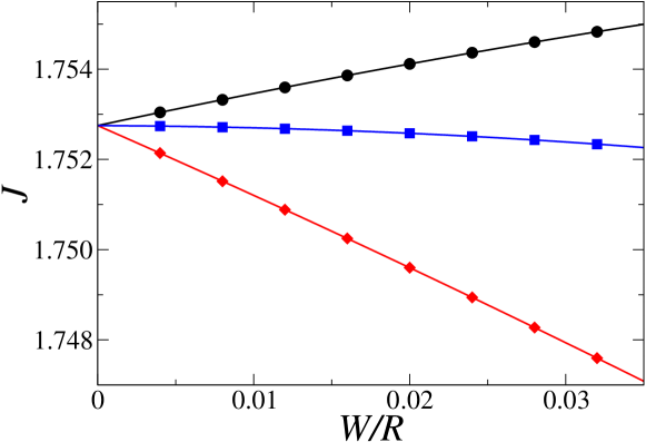
Figure 1: (Color online) Total current as function of the ratio between the interface thickness and the radius of the circle in the cases of direct (black circles), inverse (red diamonds), and tensorial (blue squares) interpolation. We solve the spherical inclusion problem with parameters: $M_{1}=1$, $M_{2}=1/2$, $R=0.25$, $h=10^{-3}$, and $\rho=10^{-6}$. Lines are obtained by quadratic regression of the simulation data (see the main text for further details). The coefficients of these regressions are contained in Tab. 1. All units are arbitrary.

2 Analysis

2.1 Problem formulation

All the problems listed above have a common structure, namely, the flux of a conserved quantity is driven by a potential gradient,

$$\bi{j}=-M(\phi)\nabla V,$$ (1)

where $V$ is a potential. The structure of Eq. (1) is standard in out-of-equilibrium thermodynamics: a linear relationship between a flux and a thermodynamic driving force (the potential gradient). The mobility coefficient $M(\phi)$ depends on the phase field $\phi$. If the transport process is electric conduction, $V$ is the electrostatic potential and $M$ the conductivity; for diffusive mass transport $V$ is the chemical potential and $M$ the atomic mobility.

The transported quantity satisfies a conservation law, which is valid both in the bulk and at the surfaces, and for a time-independent solution (steady-state flow) reads

$$\nabla\cdot\bi{j}=0.$$ (2)

The problem specification is completed by a boundary condition for the potential at the interfaces. We assume continuity of the potential,

$$V_{+}=V_{-},$$ (3)

where $V_{+}$ and $V_{-}$ are the values of the potential when the interface is approached from the two sides. This corresponds to a rapid exchange of the transported quantity between the two sides of the interface.

Since we consider a fixed and immobile two-phase structure, the phase field is independent of time. We will assume that the two constant values that designate the two phases are $\phi=0$ and $\phi=1$, and that the field $\phi$ varies between these two limits continuously through a front region of width $W$. For the sake of concreteness, the reader may have in mind a sigmoid function such as $\left[1+\tanh(x/W)\right]/2$, but the explicit form of this function is not important. The only hypothesis we make is that for a straight interface, the profile of $\phi$ is odd with respect to the point $\phi=1/2$, that is, $\phi(x)=1-\phi(-x)$ for an interface centered at $x=0$. This is the case in all standard phase-field models.

interpolation type	$J_{0}$	$c_{1}$		$c_{2}$
direct	1.752751	$0.73889\times$	$10^{-1}$	-0.277364
inverse	1.752751	$-1.51884\times$	$10^{-1}$	-0.289096
tensorial	1.752749	$-1.352\times$	$10^{-3}$	-0.358637

Table 1: Coefficients of the second order regression $J(\epsilon)=J_{0}+c_{1}\epsilon+c_{2}\epsilon^{2}$ for the three different interpolation methods. These coefficients are obtained from a quadratic regression to the data indicated by the symbols of Fig. 1.

2.2 Surface current

For simplicity of exposition, it is useful to focus on a concrete example. Consider the conduction of electric current through a two-phase material. Then, $V$ is the electrostatic potential, and $M(\phi)$ is the phase-dependent electric conductivity. Furthermore, consider a straight interface normal to the $x$ direction, centered at $x=0$. A potential gradient along the $y$ direction (along the interface) is imposed by sandwiching the material between two parallel plates located at $\pm L/2$ that are held at constant potentials $\pm U$. Since the phase field $\phi$ and hence the conductivity $M$ are constant along any line of constant $x$ (although their values differ for different values of $x$), Eq. (2) yields a constant potential gradient $U/L$ directed along the $y$ direction. Therefore, the total current $J$ that flows between the two plates is given by

$$J=\int_{-\infty}^{\infty}M(\phi)\dfrac{U}{L}\;dx.$$ (4)

Since we have considered a sample that extends to infinity, this current is clearly infinite. However, we will be concerned only with the excess of this current with respect to the sharp-interface value. The latter is obtained as the current that would flow if $\phi(x)$ was a step function, that is, the space between the two plates is filled with material 1 of conductivity $M_{1}$ for $x<0$, and with material 2 of conductivity $M_{2}$ for $x>0$. This yields

$$\bar{J}=\int_{-\infty}^{0}M_{1}\dfrac{U}{L}\;dx+\int_{0}^{\infty}M_{2}\dfrac{U}{L}\;dx.$$ (5)

The difference between these two expressions is the excess of current $\delta J$ due to the variation of conductivity over a zone of finite thickness. This excess

$$\delta J=\int_{-\infty}^{0}\hskip-7.0pt\left[M(\phi)-M_{1}\right]\dfrac{U}{L}\;dx+\int_{0}^{\infty}\hskip-7.0pt\left[M(\phi)-M_{2}\right]\dfrac{U}{L}\;dx,$$ (6)

is localized in the interface, and can therefore be interpreted as a additional current along the surface. It can be written as the product of the potential gradient and a surface conductivity

$$M_{s}=\int_{-\infty}^{0}\hskip-2.0pt\left[M(\phi)-M_{1}\right]\;dx+\int_{0}^{\infty}\hskip-2.0pt\left[M(\phi)-M_{2}\right]\;dx.$$ (7)

This surface transport coefficient has two obvious properties: (i) for an interface profile of fixed functional form, $\phi(x)=f(x/W)$, $M_{s}$ is proportional to the interface thickness (as can be shown by a simple change of variables), and (ii) it is strictly zero for any value of $W$ if

$$\int_{0}^{-\infty}\left[M(\phi)-M_{1}\right]\;dx=\int_{0}^{\infty}\left[M(\phi)-M_{2}\right]\;dx.$$ (8)

In this case, the excesses of current on the two sides of the interface exactly compensate. For a phase-field profile that satisfies $\phi(-x)=1-\phi(x)$, this can be simply achieved by choosing

$$M(\phi)=M_{1}\phi+M_{2}(1-\phi).$$ (9)

This will be called direct interpolation in the following.

2.3 Surface resistance

Let us now analyze again a planar interface normal to the $x$ direction, but this time crossed by a steady current $J_{\perp}$ along $x$. In this case, the continuity equation immediately yields that the current is constant (independent of $x$). Then, the potential $V$ satisfies the simple equation

$$-M(\phi)\partial_{x}V=J_{\perp}.$$ (10)

Integration along $x$ yields

$$V(x)-\overline{V}=-\int_{0}^{x}\frac{J_{\perp}}{M(\phi)}\;dx,$$ (11)

where $\overline{V}$ is the potential at $x=0$ (an integration constant). In contrast, if the interface was sharp, the potential would simply be given by

$$V_{0}(x)-\overline{V}=-\frac{xJ_{\perp}}{M_{1,2}}$$ (12)

for $x>0$ and $x<0$, respectively. Of course, outside the diffuse interfaces, the slopes of $V(x)$ are identical in Eqs. (11) and (12). Therefore, the asymptote of the diffuse-interface expression is of the form

$$V(x)-\overline{V}\approx-\frac{xJ_{\perp}}{M_{1,2}}+V_{+,-}$$ (13)

for $x\to\pm\infty$. The constants $V_{+}$ and $V_{-}$ (the interface potentials “seen” from the region outside the diffuse interface) are readily obtained from the matching of this expression to Eq. (11),

$$V_{+,-}=\overline{V}+J_{\perp}\int_{0}^{\infty,-\infty}\left[\frac{1}{M(\phi)}-\frac{1}{M_{1,2}}\right]\;dx.$$ (14)

Of particular interest is the fact that these surface potentials can be different, in contradiction to the assumption of Eq. (3). The difference $\delta V=V_{+}-V_{-}$ can be written as the product of the current $J_{\perp}$ and an interface resistance

$$R_{s}=\int_{-\infty}^{0}\left[\frac{1}{M(\phi)}-\frac{1}{M_{1}}\right]\;dx+\int_{0}^{\infty}\left[\frac{1}{M(\phi)}-\frac{1}{M_{2}}\right]\;dx.$$ (15)

This resistance is often called Kapitza resistance and has been frequently observed in experiments and simulations [19, 20, 21, 22, 23]. Again, it is obvious that it is proportional to the interface thickness, and that it vanishes if the integral is exactly zero. This can be achieved for any value of $W$ by the interpolation

$$\frac{1}{M(\phi)}=\frac{1}{M_{1}}\phi+\frac{1}{M_{2}}(1-\phi).$$ (16)

This will be called inverse interpolation in the following.

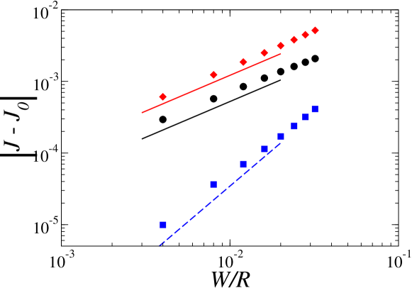
Figure 2: (Color online) Rate of convergence of the three interpolations as function of the ratio between the interface thickness and the radius of the disk. Black circles, red diamonds, and blue squares stand for direct [Eq. (9)], inverse [Eq. (16)], and tensorial interpolation [Eq. (17)], respectively. The physical and numerical parameters are the same used in Fig. 1 and $J_{0}=1.75275$. Red and black solid lines are guide to eye with slope equal to $1.0$, while blue dashed line has slope equal to $2.0$. All units are arbitrary.

2.4 Tensorial mobility

In summary, the two interface effects (surface current and surface resistance) can each be eliminated by a specific choice for the interpolation function of the mobility. Since these interpolations are mutually exclusive, it seems as if necessarily one of the two effects must remain nonzero. However, the current is a vector quantity, and the two effects are linked to distinct components of the current vector: the excess surface conductivity is relevant only for the components parallel to an interface, whereas the surface resistance modifies the boundary conditions for the normal component. Inside the two phases, where each medium is isotropic, the Curie principle requires to choose a scalar mobility to relate the current and the potential gradient. However, in the presence of an interface, isotropy of space is broken and a tensorial transport coefficient is permitted. Indeed, the gradient of the phase field can be readily used to define the interface normal $\bi{n}=\nabla\phi/|\nabla\phi|$, which provides a second direction that is independent of the potential gradient. Then, we can define the transport coefficient by

$$\bi{M}(\phi)=M_{\perp}\bi{n}\otimes\bi{n}+M_{||}(\mathbf{1}-\bi{n}\otimes\bi{n}),$$ (17)

where $\mathbf{1}$ is the unit tensor, with two independent interpolation functions $M_{\perp}(\phi)$ and $M_{||}(\phi)$. If we interpolate $M_{\perp}$ according to Eq. (16) and $M_{||}$ according to Eq. (9), both thin-interface effects are eliminated. Hence, for this interpolation the transport problem defined by Eq. (1) becomes

$$\bi{j}=-\bi{M}(\phi)\cdot\nabla V,$$ (18)

with components (in two dimensions)

$$j_{x} = M_{xx}\partial_{x}V+M_{xy}\partial_{y}V,$$ (19)

$$j_{y} = M_{xy}\partial_{x}V+M_{yy}\partial_{y}V.$$ (20)

Here, we have designated by $M_{ij}$ the elements of the symmetric tensor $\bi{M}(\phi)$. The simple calculations developed above are valid only for planar interfaces. However, for a sufficiently smooth interface (that is, with a local radius of curvature $R$ satisfying $R\gg W$), a local curvilinear coordinate system can be defined in which the above relations remain valid at least up to second order in $\epsilon=W/R$. It should be mentioned that a similar strategy has been used recently to develop efficient phase-field models for surface diffusion [24].

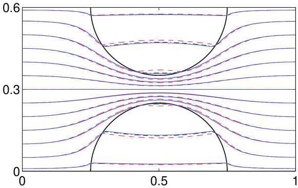
Figure 3: (Color online) Streamlines for the second geometrical configuration studied. The black dash-dotted, red dashed, and blue solid lines correspond to direct, inverse, and tensorial interpolation, respectively. The simulation parameters are $M_{1}=1$, $M_{2}=0.1$, $R=0.25$, $h=10^{-3}$, $\rho=10^{-6}$, and $W=4h$. For a larger version of this picture see [25]. All units are arbitrary.

3 Numerical validation

We quantify the thin-interface effects in the three different interpolations of the transport coefficient by solving the problem defined by Eq. (1) [or (18)] and Eq. (2) in a simple geometrical setup. We consider a square domain ${\cal D}\equiv\{(x,y)\in[0,1]\times[0,1]\}$ with Dirichelet boundary conditions on the lateral edges and zero flux at the upper and bottom edges. More precisely, we impose $V(0,y)=1$, $V(1,y)=-1$, and $\partial_{y}V(x,0)=\partial_{y}V(x,1)=0$. In the center of the domain we place a disk of radius $R$. The mobility coefficient takes a value of $M_{1}$ ($M_{2}$) outside (inside) the disk, respectively. We refer to this geometrical setup as spherical inclusion problem.

By combining the flux equation Eq. (1) [or its tensorial counterpart (18)] with the conservation law of our problem, i.e.  Eq. (2), we obtain an elliptic equation for the case of direct and inverse interpolation

$$\nabla\cdot\left[M(\phi)\,\nabla V\right]=0,$$ (21)

whereas the tensorial interpolation leads to the following equation

$$\nabla\cdot\left[\bi{M}(\phi)\cdot\nabla V\right]=0.$$ (22)

Details about the discretization and the method used to solve these equations can be found in the appendix.

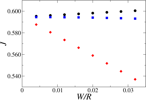
Figure 4: (Color online) Total current as function of the ratio between the interface thickness and the radius of the circle for direct (black circles), inverse (red diamonds), and tensorial (blue squares) interpolations. The simulation parameters are the same of Fig. 3. All units are arbitrary.

The thin-interface effects arising in the spherical inclusion problem are quantified by measuring the total flux at $x=1$,

$$J=\int_{0}^{1}j_{x}(1,y)\,dy$$ (23)

and by plotting $J$ as a function of the ratio $\epsilon=W/R$ between the interface width $W$ and the radius of the disk $R$, see Fig. 1. As shown in Fig. 1, the three interpolations converge to the same value of $J_{0}$ when $\epsilon\to 0$. The estimation of $J_{0}$ is given by a quadratic regression in $\epsilon$ of the simulation data. The coefficients of the regressions are listed in Table 1. Within the truncation error [that is ${\rm O}\left(h^{2}\right)\sim 10^{-6}$] the three interpolations give the same value of $J_{0}=1.752750\pm 10^{-6}$, as shown in the second column of Table 1.

In addition, we have estimated the rate of convergence of $J(\epsilon)$ to the sharp-interface limit $J_{0}$ for the three interpolations of the mobility. As shown in Fig. 2, the direct and inverse interpolations converge only linearly with $\epsilon$ to this limiting value, whereas the tensorial interpolation suppress linear thin-interface effects, which leads to a convergence that is almost quadratic in $\epsilon$.

For further illustration, we consider a second geometrical configuration formed by two half-disks of radius $R$ placed in a rectangular domain with the same boundary condition of the spherical inclusion problem, see Fig. 3. We choose a small value of the ratio between $M$ inside and outside the half-disks, e.g. $M_{2}/M_{1}=0.1$, and in Fig. 3 we plot the streamlines for this configuration. In this configuration, the flux is constricted in the narrow space between the two half disks. The difference between the three interpolations is largest for streamlines which are locally almost tangent to the half-disks; note the divergence of the different lines close to the tips of the half-disks. As shown by Eq. (8), choosing $M$ according to the direct interpolation cancels exactly the surface conductivity $M_{s}$ for a flat interface. Therefore, thin-interface errors affecting streamlines which are parallel to the boundary of variation of the transport coefficient are more pronounced in case of inverse interpolation (red dashed lines) than in case of direct interpolation (black dash-dotted lines), see Fig. 3. In Fig. 4, we show again the values of the total current as a function of the ratio $\epsilon$, and again the tensorial interpolation performs much better than the other two, as expected.

4 Conclusion

We have investigated a phase-field model with a mobility tensor, in which normal and parallel components of the flux are interpolated with distinct functions of the phase field. Contrary to phase-field models with scalar mobilities, this method makes it possible to eliminate at the same time the additional surface diffusion and the surface resistance, which are both linked to the finite thickness of the interfaces. This opens the possibility to perform accurate simulations of two-phase transport problems with enlarged interface thickness, which can lead to dramatic savings in computation time.

The complete elimination of thin-interface effects to first order in the interface thickness is also a prerequisite for the development of a quantitative crystal growth model for arbitrary ratio of the diffusion coefficients in the two phases. Indeed, a tensorial diffusion coefficient can remove both surface diffusion and the Kapitza resistance [12] from such models. Even if a second order asymptotic analysis of a time dependent version of the tensorial problem (17) has been recently performed [26], this methodology is still not capable of removing all thin-interface effects from phase-field models with a non-stationary $\phi$. The obstacle that needs to be overcome for the successful development of such a model is to find a coupling of the transport equation to an evolution equation for the phase field that yields the correct boundary conditions for the transport field at moving interfaces. We hope to be able to report on this problem in the near future.

Numerical Methods

The differential operators involved in Eq. (21) and (22) are approximated by finite differences. The domain $\cal D$ is discretized by an uniform square mesh with elements of area $h^{2}$. The fields $M$, $V$, $j_{x}$, and $j_{y}$ are placed in different grids according to the standard marker and cell (MAC) method [27]. In the primary grid we locate $\phi$, $M$ ($M_{xx}$ and $M_{yy}$ in case of tensorial interpolation), and $V$ while in the two staggered grids (one for each direction) we put each component of the flux $\bi{j}$. The primary nodes $(i,j)$ have coordinates

$$x = h(i+1/2),$$ (24)

$$y = h(j+1/2),$$ (25)

whereas the two staggered grids are shifted of $h/2$ in the $x$ ($y$) direction for $j_{x}$ ($j_{y}$), respectively. In what follows, with the notation $[\dots]_{i,j}$ we mean that the field inside square brackets is evaluated at the position $(i,j)$ with respect to the primary grid. For example, at the nodes of the $x$ staggered grid we have $j_{x\,i,j}$ that is the value of $x$ component of the flux between the nodes $(i,j)$ and $(i+1,j)$ of the primary grid, i.e. $\left[Êj_{x}\right]_{i+1/2,j}$.

In order to compute $\bi{j}$ with this MAC arrangement we have to specify the values of $M$ at the nodes of the staggered grids. This is readily done by using the averaging operator on the $k$ coordinate $\mu^{\pm}_{k}$, that is

$$\left[M\right]_{i\pm 1/2,j}=\mu^{\pm}_{x}M_{i,j}=\left(M_{i\pm 1,j}+M_{i,j}\right)/2,$$ (26)

$$\left[M\right]_{i,j\pm 1/2}=\mu^{\pm}_{y}M_{i,j}=\left(M_{i,j\pm 1}+M_{i,j}\right)/2.$$ (27)

Hence, the two components of the flux $\bi{j}$ read

$$j_{x\,i,j}=\left[j_{x}\right]_{i+1/2,j}=\mu^{+}_{x}M_{i,j}\,\triangle^{+}_{x}V_{i,j}/h,$$ (28)

$$j_{y\,i,j}=\left[j_{y}\right]_{i,j+1/2}=\mu^{+}_{y}M_{i,j}\,\triangle^{+}_{y}V_{i,j}/h,$$ (29)

where $h^{-1}\triangle^{+}_{k}$ is the standard forward difference operator acting on the $k$ direction. Finally, Eq. (21) is discretized by employing the backward difference operators $h^{-1}\triangle^{-}_{k}$

$$\dfrac{1}{h^{2}}\sum_{k=x,y}\triangle^{-}_{k}\left(\mu^{+}_{k}M_{i,j}\,\triangle^{+}_{k}V_{i,j}\right)=0.$$ (30)

Evidently, the discretization of the elliptic problem arising from the tensorial interpolation $\bi{M}$ is more involved. In fact, two parts of Eq. (22) mix $x$ and $y$ derivatives, i.e. $\partial_{x}\left(M_{xy}\partial_{y}V\right)$ and $\partial_{y}\left(M_{xy}\partial_{x}V\right)$. In order to guarantee second order accuracy and maximum compactness of the discrete stencil it is convenient to place the $M_{xy}$ component of the tensor $\bi{M}$ on a third grid, whose nodes are shifted by $h/2$ in the two directions [28]. The tensorial interpolation produces an additional contribution to $j_{x}$

$$\left[M_{xy}\partial_{y}V\right]_{i+1/2,j}=\mu_{y}^{-}\left(M_{xy\,i,j}\mu_{x}^{+}\triangle^{+}_{y}V_{i,j}\right)/h,$$ (31)

and to $j_{y}$

$$\left[M_{xy}\partial_{x}V\right]_{i,j+1/2}=\mu_{x}^{-}\left(M_{xy\,i,j}\mu_{y}^{+}\triangle^{+}_{x}V_{i,j}\right)/h.$$ (32)

As before, by applying backward differentiation we obtain the discrete version of Eq. (22)

$$\begin{split}\frac{1}{h^{2}}&\Big{\{}\triangle^{-}_{x}\left[\mu^{+}_{x}M_{xx\,i,j}\,\triangle^{+}_{x}V_{i,j}+\mu_{y}^{-}\left(M_{xy\,i,j}\mu_{x}^{+}\triangle^{+}_{y}V_{i,j}\right)\right]+\\ &\triangle^{-}_{y}\left[\mu_{x}^{-}\left(M_{xy\,i,j}\mu_{y}^{+}\triangle^{+}_{x}V_{i,j}\right)+\mu^{+}_{y}M_{yy\,i,j}\,\triangle^{+}_{y}V_{i,j}\right]\Big{\}}=0.\end{split}$$ (33)

The MAC arrangement ensures a second order accuracy of the truncation error of the two elliptic problems [27, 28]. Eq. (30) and (33) are two linear systems of equations where the unknowns are the values of the potential $V_{i,j}$. These linear systems can be easily solved through any iterative method, for example by the Successive Over Relaxation (SOR) [29]. To find an accurate solution of these problems we iterate the SOR algorithm until the maximum residue at the nodes of the primary grid

$$\rho=\max_{i,j}\big{|}\left[\nabla\cdot\bi{j}\right]_{i,j}\big{|},$$ (34)

is comparable with the truncation error, i.e. $\rho\leq h^{2}$.

References

- [1] W. J. Boettinger, J. A. Warren, C. Beckermann, and A. Karma. Phase-field simulation of solidification. Annu. Rev. Mater. Res., 32:163–194, 2002.
- [2] I. Steinbach. Phase-field models in materials science. Model. Simul. Mater. Sci. Eng., 17(7):073001, 2009.
- [3] D. M. Anderson, G. B. McFadden, and A. A. Wheeler. Diffuse-interface methods in fluid mechanics. Annual Review of Fluid Mechanics, 30:139, 1998.
- [4] L.-Q. Chen. Phase-field models for microstructure evolution. Annu. Rev. Mater. Res., 32:113, 2002.
- [5] Y. Wang and J. Li. Phase field modeling of defects and deformation. Acta Mater., 58:1212–1235, 2010.
- [6] A. Karma and W.-J. Rappel. Quantitative phase-field modeling of dendritic growth in two and three dimensions. Phys. Rev. E, 57(4):4323–4349, 1998.
- [7] R. F. Almgren. Second-order phase field asymptotics for unequal conductivities. SIAM J. Appl. Math., 59:2086–2107, 1999.
- [8] A. Karma. Phase-field formulation for quantitative modeling of alloy solidification. Phys. Rev. Lett., 87(10):115701, 2001.
- [9] B. Echebarria, R. Folch, A. Karma, and M. Plapp. Quantitative phase-field model of alloy solidification. Phys. Rev. E, 70(6):061604, 2004.
- [10] R. Folch and M. Plapp. Quantitative phase-field modeling of two-phase solidification. Phys. Rev. E, 72(1):011602, 2005.
- [11] M. Ohno and K. Matsuura. Quantitative phase-field modeling for dilute alloy solidification involving diffusion in the solid. Phys. Rev. E, 79(3):031603, 2009.
- [12] M. Plapp. Remarks on some open problems in phase-field modelling of solidification. Phil. Mag., 91:25–44, 2011.
- [13] J. Kockelkoren, H. Levine, and W.-J. Rappel. Computational approach for modeling intra- and extracellular dynamics. Phys. Rev. E, 68:037702, Sep 2003.
- [14] Flavio H. Fenton, Elizabeth M. Cherry, Alain Karma, and Wouter-Jan Rappel. Modeling wave propagation in realistic heart geometries using the phase-field method. CHAOS, 15(1):013502, 2005.
- [15] Alfonso Bueno-Orovio, V団tor M. P屍ez-Garc誕, and Flavio H. Fenton. Spectral methods for partial differential equations in irregular domains: The spectral smoothed boundary method. SIAM J. Sci. Comput., 28(3):886–900, 2006.
- [16] X. Li, A. Ratz, and A. Voigt. Solving pdes in complex geometries: A diffuse domain approach. Comm. Math. Sci., 7:81, 2009.
- [17] M. Benes, V. Chalupecký, and K. Mikula. Geometrical image segmentation by the Allen-Cahn equation. Appl. Numer. Math., 51:187–205, 2004.
- [18] D. A. Kay and A. Tomasi. Color Image Segmentation by the Vector-Valued Allen-Cahn Phase-Field Model: A Multigrid Solution. IEEE Trans. Image Process., 18:2330–2339, 2009.
- [19] P. L.Kapitza. Unknown. Zh. Eksp. Teor. Fiz., 11:1, 1941.
- [20] P. E. Wolf, D. O. Edwards, and S. Balibar. MEASUREMENTS OF THE KAPITZA RESISTANCE AND ONSAGER CROSS-COEFFICIENT FOR THE HE-4 CRYSTAL SUPERFLUID INTERFACE. J. Low Temp. Phys., 51(5-6):489–504, 1983.
- [21] E. T. Swartz and R. O. Pohl. Thermal boundary resistance. Rev. Mod. Phys., 61(3):605–668, Jul 1989.
- [22] J.-L. Barrat and F. Chiaruttini. Kapitza resistance at the liquid-solid interface. Mol. Phys., 101(11):1605–1610, 2003.
- [23] L. Xue, P. Keblinski, S. R. Phillpot, S. U.-S. Choi, and J. A. Eastman. Two regimes of thermal resistance at a liquid–solid interface. J. Chem. Phys., 118(1):337–339, 2003.
- [24] C. Gugenberger, R. Spatschek, and K. Kassner. Comparison of phase-field models for surface diffusion. Phys. Rev. E, 78:016703, 2008.
- [25] See supplementary material at XXXX for a larger version of Fig. 3.
- [26] T. P. Ngoc, and M. Plapp, unpublished.
- [27] C. Pozrikidis. Introduction to Theoretical and Computational Fluid Dynamics. Oxford University Press, New York, 1997.
- [28] Marc Gerritsma. Time dependent numerical simulations of a viscoelastic fluid on a staggered grid. Ph.D. thesis, Groningen, Netherlands, 1996.
- [29] W. H. Press, S. A. Teukolsky, W. T. Vetterling, and B. P. Flannery. Numerical Recipes 3rd edition: The art of scientific computing. Cambridge University Press, Cambridge, 2007.