Quantum superposition of three macroscopic states
and superconducting qutrit detector

Abstract

Superconducting quantum coherent circuits have opened up a novel area of fundamental low-temperature science since they could potentially be the element base for future quantum computers. Here we report a quasi-three-level coherent system, the so-called superconducting qutrit, which has some advantages over a two-level information cell (qubit), and is based on the qutrit readout circuit intended to measure individually the states of each qubit in a quantum computer. The designed and implemented radio-frequency superconducting qutrit detector (rf SQUTRID) with atomic-size ScS-type contact utilizes the coherent-state superposition in the three-well potential with energy splitting $\Delta E_{01}/k_{B}\approx 1.5\,$K at the 30th quantized energy level with good isolation from the electromagnetic environment. The reason why large values of $\Delta E_{01}$ (and thus using atomic-size Nb-Nb contact) are required is to ensure an adiabatic limit for the quantum dynamics of magnetic flux in the rf SQUTRID.

I Introduction

The phenomenon of the superposition of states of a macroscopic object predicted for a superconducting quantum interferometer device (SQUID) in the low-dissipation limit1 ; 2 ; 3 was revealed in spectroscopic experiments.4 ; 5 Although much progress has been made in demonstrating the coherent quantum behavior of various systems with Josephson junctions,6 there has not been an experimental presentation of a readout device based on the quantum superposition of macroscopically distinct states in flux qubits. The dependence of this fundamental property of quantum mechanics, the superposition of states, on the symmetry of the potential energy in flux qubits can be taken as a basis for creating a radio-frequency superconducting qubit detector (rf SQUBID) similar to the manner of how the Josephson current-phase relation is used in building rf SQUIDs.7 This device would be a principal element in quantum readout circuits meant for weak continuous measurement of states of the flux qubits incorporated in the quantum computer architecture.

However, there is a pitfall on this way. In the literature, the flux qubit (a superconducting ring closed by a superconductor-insulator-superconductor (SIS) junction) is described as the superposition of the two states $\left|\Psi\right\rangle=c_{1}(t)\left|\Psi_{1}\right\rangle+c_{2}(t)\left|\Psi_{2}\right\rangle$ that appear in this quantum system with double-well potential. If the tunneling amplitude is large (in other words, if coefficients $c_{1}$ and $c_{2}$ vary quickly enough), the system behavior becomes adiabatic when changing the external magnetic flux; that is, it can be considered in terms of quasi-stationary superposition levels. In this case, it becomes impossible to distinguish between the experimental characteristics of a common classical SQUID in a nonhysteretic regime and a double-well SQUBID. Both devices behave as parametric inductances (Josephson inductance for SQUID and quantum inductance for SQUBID), with both inductances being maximized at the same external flux, $\Phi_{e}=(n+1/2)\Phi_{0}$ (where $n$ is an integer and $\Phi_{0}=h/2e$ is the superconducting flux quantum), so that some additional evidence is required for establishing the quantum nature of the object under study. Unlike this situation, with the superposition of three classically separated states in the superconducting ring, the characteristics of a radio-frequency superconducting qutrit detector (rf SQUTRID) will possess essential distinctions8 , allowing one to state definitely their quantum origin. Particularly, the quantum inductance extrema in the qutrit should be observed at external magnetic flux $\Phi_{e}=n\Phi_{0}$.

Here we present experimental evidence and a theoretical analysis for the fact that a rf SQUID with atomic-size ScS contact can be put into superposition of three distinct states with a macroscopically large time of energy relaxation to lower levels and thus be turned into a rf SQUTRID. We explore the voltage-current and voltage-flux (signal) characteristics of this new device for the first time. Note that in the qutrit we study, the superposition states are formed due to the fast tunneling of flux through potential barriers in the triple-well symmetrical potential in the phase space and the removal of the degeneracy of states of equal energy in each well, unlike in Ref. QT, , where the transmon with its three lowest energy levels was used as a qutrit whose superposition states were prepared by exciting the transmon from the base energy level to two higher ones.

A substantial difference between the Josephson properties of ScS and SIS contacts at low temperatures has been predictedQPC1 ; CPC ; QPC2 ; 10 in the microscopic theory of superconducting weak links. The singular potential corresponds to the case of a “clean” ScS contact with a dimension $d$ much smaller than the superconducting coherence length $\xi_{0}$ and the electron elastic mean free path $\ell$ (the so-called ballistic regime $d\ll\ell$). This fact leads to some peculiarities in the macroscopic quantum tunneling11 ; 12 and the quantum coherence of magnetic flux states in a superconducting ring closed by ScS contact. The major ones are an appreciable increase in the qutrit key performance parameter, the splitting of degenerate energy levels in separate potential wells,8 and the emergence of high nonlinearity in the resulting qutrit superpositional levels that can be used in the rf SQUTRID based on rf SQUID circuitry (Fig. 1).

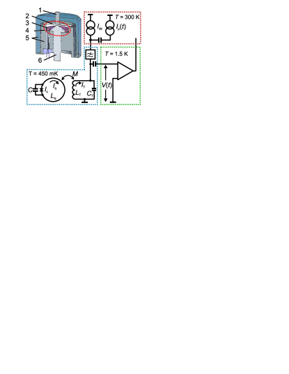
Figure 1: (Color online) Circuit diagram of the SQUTRID. Experimental set-up is characterized by the following parameters: $L_{T}=1.2\,\mu$H, $C_{T}=630$ pF, $I_{P}(t)=I_{0}\cos\omega t$, $\omega_{T}/2\pi=5.794$ MHz, $Q=302$, $M=k\sqrt{L_{q}L_{T}}=1.52$ nH, and $L_{q}=0.3$ nH; the qutrit values $I_{c}$ and $C$ are discussed in the text. The inset shows the fully niobium 3D toroidal construction of the qutrit cell, where 1 is the pusher, 2 is the membrane, 3 is a part of the $L_{T}$ coil, 4 is the toroidal quantization loop (cavity), 5 is the body, and 6 is the needle.

II The SQUTRID model

Currently, two types of point contacts are distinguished, depending on the ratio between the contact dimension $d$ and the electron wave length $\lambda_{F}=h/p_{F}$: $d\gg\lambda_{F}$ for a classical point contact and $d\sim\lambda_{F}$ for a quantum point contact.QPC1 In metals, actually, a quantum point contact is necessarily of atomic dimensions, as the electron wave length is of the same order of magnitude as the atomic separation. For both classicalCPC and quantumQPC2 ScS point contact with the critical current $I_{c}$, at $T=0$ the current-phase relation reads

$$\begin{array}[]{c}\displaystyle{I_{s}(\varphi)=I_{c}\sin\frac{\varphi}{2}\,\textrm{sgn}[\cos\frac{\varphi}{2}],\,\,I_{c}=\frac{\pi\Delta_{0}}{eR_{N}},}\end{array}$$ (1)

where $\Delta_{0}$ is the superconducting energy gap and $R_{N}$ is the normal-state resistance of ScS contact. The critical current of the atomic-size (quantum) ScS contact was predictedQPC2 to be quantized (as a consequence of the quantization of the contact conductance $R_{N}^{-1}$, in units of $G_{0}=2e^{2}/h$), $\displaystyle{I_{c}=N(e\Delta_{0}/\hbar)}$, which was observed experimentally.QPC1 From (1) one gets the Josephson coupling energy of ScS contact in the form $U_{J}=-(I_{c}\Phi_{0}/\pi)|\cos(\varphi/2)|$.

To develop the SQUTRID model in a zero-temperature approximation, we take the quantum Hamiltonian in the flux representation of the superconducting loop (Fig. 1) of inductance $L_{q}$ closed by a clean atomic-size ScS contact with critical current $I_{c}$ and self-capacitance $C$ (so that parameter $g=E_{J}/E_{C}=\Phi_{0}I_{c}C/(2\pi e^{2})\gg 1$) in the form8 ; 11 ; 12 ; 13

$$\begin{array}[]{c}\displaystyle{\hat{H}_{q}=\frac{\hat{P}^{{\rm 2}}}{{\rm 2}M}+\hat{U}(f;f_{e})=\vspace{2mm}}\\ \displaystyle{=-\frac{\hbar^{2}}{2M}\frac{\partial^{2}}{\partial f^{2}}+{\frac{\Phi_{0}I_{c}}{2\pi}}\left[-2\left|\cos(\pi f)\right|+\frac{2\pi^{2}(f-f_{e})^{2}}{\beta_{L}}\right],\vspace{2mm}}\\ \displaystyle{M=\Phi_{0}^{2}C,\quad\beta_{L}=\frac{2\pi L_{q}I_{c}}{\Phi_{0}},}\end{array}$$ (2)

where $f=\Phi/\Phi_{0}$ and $f_{e}=\Phi_{e}/\Phi_{0}$ are the normalized internal magnetic flux $\Phi$ in the loop and external magnetic flux $\Phi_{e}$ applied to the loop. The quantum dynamical observable of the internal magnetic flux in the loop is given by an operator of flux conjugated to an operator of charge in the contact capacitance: $[\hat{\Phi},\hat{Q}]=-i\hbar$.13 The key feature of Hamiltonian (2) is its singular potential $U(f;f_{e})$ following from the nonsine current-phase relation (1) for ScS contact. Note that a model with both the potential attributed to ScS contact and the dissipation vanishing at zero temperature can satisfactorily describe the experiments on macroscopic quantum tunneling in a ring with a clean ScS contact,12 as shown in Ref. 11, .

The solutions of the stationary Schrödinger equation

$$\hat{H}_{q}(f;f_{e})\,\Psi(f)=E(f_{e})\,\Psi(f)$$ (3)

with Hamiltonian (2) yield wave functions $\Psi(f)$ and energies $E(f_{e})$ of the stationary states of the superconducting loop with ScS contact at a specified external magnetic flux $f_{e}$. Let us consider the SQUTRID superconducting loop where a three-well potential is formed. We get a series of states appeared during fast (with rf generator rate $\omega$) increasing of external flux $\Phi_{e}$ from 0 to $\Phi_{0}$ (Fig. 2) using parameters in Eq. (3) close to our experimental values: $L_{q}=0.3$ nH, $C=4.36$ fF, and $\beta_{L}=4.0$ ($I_{c}\approx 4.4\,\mu$A). It is seen from these solutions that, with a change in external flux, the initial state of a three-well symmetrical potential localized in the central well at $\Phi_{e}=0$ [Fig. 2(a)] transforms through intermediate states [Fig. 2(b) and 2(c)] into a superposition state in a three-well symmetrical potential at $\Phi_{e}=\Phi_{0}$ [Fig. 2(d)]. Note that the energy exchange rate between the two classically separated states in a two-well symmetrical potential at $\Phi_{e}=\Phi_{0}/2$ is exponentially small at the specified parameters, so the system state remains localized in the starting potential well during the increase in external flux toward the point $\Phi_{e}=\Phi_{0}$. In this point, the superposition qutrit state ${\left|\Psi_{S0}\right\rangle}=c_{1}{\left|\Psi_{1}\right\rangle}+c_{2}{\left|\Psi_{2}\right\rangle}+c_{3}{\left|\Psi_{3}\right\rangle}$ of the wave functions of all three separate wells is formed in the three-well symmetrical potential, similar to the formation of the superposition qubit state in the two-well potential.

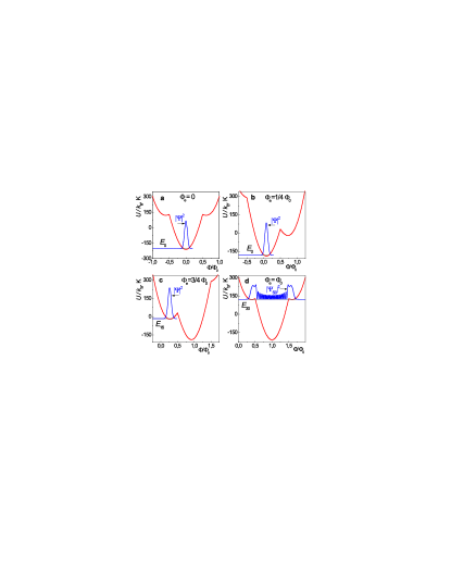
Figure 2: (Color online) Forming the base superposition SQUTRID state by rapid change of external flux $\Phi_{e}$. The set of nonstationary potential energies $U(f)/k_{B}$, in terms of temperature, and squared wave functions $\left|\Psi(f)\right|^{2}$ are shown vs normalized internal flux $f=\Phi/\Phi_{0}$ at various $\Phi_{e}$; $\beta_{L}=4.0$. Subscript after $E$ refers to the energy level number. (a) The SQUTRID is initially in its ground state; its wave function is localized in the absolute minimum of the symmetrical potential. (b) The potential becomes asymmetrical with two wells, but the system is still in its ground state, and the wave function is localized in the minimum of the deeper well. (c) The wave function remains surprisingly localized in the same single well since the potential changes too quickly in comparison with the tunneling rate (the interwell barrier is rather high in this case). (d) The base state $\left|\Psi_{S0}\right|^{2}$ of the three-well superposition is formed in the potential symmetry point when the barriers are small, and tunneling time is consequently short. The relaxation time of this state turns out to be macroscopically large, so that it becomes stable enough and “latched” for many further cycles of $\Phi_{e}$.

Quantum coherence of the qutrit flux state ${\left|\Psi_{S0}\right\rangle}$ in a three-well potential manifests itself as coherent oscillations of magnetic flux between all the three potential wells due to its fast tunneling through the potential barriers separating the central and the side wells. Numerical analysis of Eq. (3) shows that, for resonant tunneling in a three-well potential of the superconducting loop of inductance $L_{q}=0.3$ closed by a clean ScS contact with $C=3-6\,$fF ($\beta_{L}=4.0$), the flux oscillation rate between wells $\nu_{01}=\Delta E_{01}/h$ reaches $25-40$ GHz. The magnetic moment of the flux states corresponding to the side wells of the three-well potential $\mu_{s}^{(1,3)}=I_{s}S\simeq 10^{-11}$ J/T $\simeq 10^{12}\mu_{B}$ (where $I_{s}\simeq 0.6\Phi_{0}/L_{q}\approx 4\,\mu$A is the supercurrent in the side-well flux states, $S\simeq 2\!\times\!10^{-6}\,$m² is the loop area, and $\mu_{B}=0.93\!\times\!10^{-23}$ J/T is the Bohr magneton), and the magnetic moment of the central flux state $\mu_{s}^{(2)}=0$ (since the supercurrent is zero in this state). Thus, we have the coherent superposition of wave functions corresponding to the three distinct macroscopic flux states in the three-well symmetrical potential of the qutrit at $\Phi_{e}=n\Phi_{0}$.

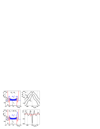
Figure 3: (Color online) Superposition of three states in the superconducting loop closed by a clean ScS contact. Distributions of squared wave functions $\left|\Psi_{S0}(f)\right|^{2}$ among the three potential wells vs normalized internal flux $f=\Phi/\Phi_{0}$ for two close values of external magnetic fluxes $\Phi_{e}$ corresponding to (a) fully symmetrical and (b) slightly tilted potential $U(f)$; $\beta_{L}=4.0$. Superposition energy levels are denoted $E_{S0},E_{S1},$ and $E_{S2}$. The process of energy relaxation of the base superposition state $\Psi_{S0}(f)$ from level $E_{S0}$ to level $E_{-1}$ with characteristic time $\tau_{\varepsilon}$ is shown by arrows. (c) Superposition energy levels $E_{S0},E_{S1},$ and $E_{S2}$ vs normalized external magnetic flux $f_{e}=\Phi_{e}/\Phi_{0}$. (d) Normalized quantum inductance of the base superposition level $E_{S0}$ vs $f_{e}$: curve 1 is zero-noise $(L_{q}L_{Q}^{-1})(f_{e})$ and curve 2 is noise-affected $(L_{q}L_{Q}^{-1})_{eff}(f_{e})$ averaged over low-frequency noise with $\sigma=\sqrt{\left\langle\delta f_{e}^{2}\right\rangle}=0.013$.

Let us refer to ${\left|\Psi_{S0}\right\rangle}$, which is the three-well superposition state with minimum energy, as the “base” SQUTRID superposition state since adiabatic movement along the respective energy level $E_{S0}$ plays the main role in our experiments. State ${\left|\Psi_{S0}\right\rangle}$ in the potential $U(f;f_{e})$ is characterized by quantum number $n\gg 1$ [$n=30$ for the above-cited parameter values; see Fig. 2(d)]; i.e., the deep central well ($\Delta U/k_{B}\simeq 300$ K) contains a large number of quantum levels. The time $\tau_{\varepsilon}$ of the energy relaxation of the base SQUTRID state to underlying states in the central well must be macroscopically large to enable measuring the superpositional nonlinearity. This is achieved due to the design of the qutrit loop in the form of a high-quality three-dimensional (3D) toroidal superconducting cavity (see inset in Fig. 1 and Sec. III), which has no resonant modes with frequencies corresponding to the frequencies (energies) of transitions from the base superpositional level $E_{S0}$ to underlying energy levels.

Figure 3(a) displays numeric solutions of Eq. (3) for the squared absolute value of the wave function of the base superposition state $|\Psi_{S0}(f)|^{2}$ and energy levels $E_{S0},E_{S1}$, and $E_{S2}$ of the three superposition states as well. The fact that splitting $\Delta E_{01}/k_{B}=(E_{S1}-E_{S0})/k_{B}=1.65$ K between the base and the nearest superposition energy levels substantially exceeds the environment temperature for the chosen parameters is key in the present experiment ($\Delta E_{01}/k_{B}T=1.65/0.45\approx 3.7$). As a result, the broadening of level $E_{S0}$ because of statistical averaging over equilibrium density matrix $\delta E_{S0}=\Delta E_{01}/[1+\exp(\Delta E_{01}/k_{B}T)]\ll\Delta E_{01}$ is relatively small ($\delta E_{S0}/k_{B}\approx 0.04$ K) and can be neglected in the analysis of the system energy structure (zero-temperature approximation). Also, it is obvious that the large tunnel splitting, which multiply overruns the temperature value, guarantees good “quantumness” of the superconducting loop closed by a clean ScS contact provided that the environment and the measurement circuit noises are effectively suppressed. At the same time, the base superposition level $E_{S0}$ is situated far below the potential barrier top $U_{b}$, $(U_{b}-E_{S0})/k_{B}\approx 5$ K$\,\,\gg T$, so that thermal transitions rate over the barrier is vanishingly small, and the process of relaxation of the metastable base superposition state into the deep central well can be strongly limited for the chosen parameters since $(E_{S0}-E_{-1})/k_{B}\approx 8$ K.

Small adiabatic variations of the external flux relative to symmetry points $\Phi_{e}=n\Phi_{0}$ lead to tilting the three-well potential, with a change in the wave functions and the energy levels. As seen from Fig. 3b, when the flux shifts apart from the symmetry point $\Phi_{e}=\Phi_{0}$, the wave packet of the base state $|\Psi_{S0}(f)|^{2}$ partially transfers into the deeper side potential well. A rearrangement of the superposition wave packets and thus the formation of the superposition energy levels $E_{S0}(f_{e}),E_{S1}(f_{e})$ and $E_{S2}(f_{e})$ [shown in Fig. 3(c)] occur over the time span reciprocal to the flux tunneling rate, $t_{S}\approx\nu_{01}^{-1}$ . In experiment, we deal with relatively low-frequency (adiabatic) processes, in which the time-dependent superposition levels practically coincide with the stationary ones.

The superconducting qutrit detector is built on the basis of rf SQUID circuitry. That is, the qutrit is inductively coupled to a high-quality $L_{T}C_{T}$ superconducting tank (Fig. 1) serving as a linear classical detector ($\hbar\omega_{T}\ll k_{B}T$). Only a small fraction of the flux in the $L_{T}C_{T}$ tank ($M/L_{T}\approx 0.0013$ in our experiment, where $L_{T}$ is the tank inductance and $M$ is the mutual inductance between the qutrit and the tank) is transferred to the qutrit, which allows making use of the concept of weak continuous quantum measurements.WCM1 ; WCM2 ; WCM3 When the characteristic frequency of the classical detector ($L_{T}C_{T}$ tank) is much lower than that of the quantum object (in our system the ratio $\omega/\nu_{01}\sim 10^{-3}$), the latter’s dynamics can be studied by means of quantum-mechanical equations with the detector classical field treated as the external adiabatic parameter.IMTt1 ; IMTt2 ; IMTt3 Within this semiclassical approach of treating the qutrit plus tank system, one obtains the classical equation for the $L_{T}C_{T}$ tank containing the parametric quantum inductance contribution [see Eq. (7)], instead of the parametric Josephson inductance contribution probed in rf SQUID by means of the impedance measurement technique (IMT). The IMT with a weak continuous quantum readout was successfully applied to studying different types of qubits.IMTe1 ; IMTe2 ; IMTe3

For the $L_{T}C_{T}$ tank driven by rf-bias current $I_{0}\cos\omega t$, the measured output functions are the amplitude of voltage oscillations $V_{T}$ and the voltage-current phase shift $\alpha_{T}$. The equation for voltage $V(t)$ across the $L_{T}C_{T}$ tank having the quality factor $Q=\omega_{T}R_{T}C_{T}$, with the current contribution due to the weakly coupled qutrit $MI_{q0}/L_{T}$ taken into account, reads

$$C_{T}\dot{V}+\frac{V}{R_{T}}+\frac{1}{L_{T}}\!\int\!Vdt+\frac{MI_{q0}}{L_{T}}=I_{P}(t),\,I_{P}(t)=I_{0}\cos\omega t.$$ (4)

Here

$$I_{q0}(\Phi_{e})=\frac{\partial\langle\Psi_{S0}|\hat{H}_{q}|\Psi_{S0}\rangle}{\partial\Phi_{e}}=\frac{\partial E_{S0}(\Phi_{e})}{\partial\Phi_{e}}$$ (5)

is the current circulating in the superconducting loop of the qutrit in its base quantum superposition state, as a function of the total external flux $\Phi_{e}$.

In further considerations it is convenient to use the function $L_{Q}^{-1}(f_{e})$, which is called the reciprocal quantum inductance, defined as

$$L_{Q}^{-1}(f_{e})=\frac{\partial I_{q0}(\Phi_{e})}{\partial\Phi_{e}}=\frac{\partial^{2}E_{S0}(\Phi_{e})}{\partial\Phi_{e}^{2}}=\frac{1}{\Phi_{0}^{2}}\frac{\partial^{2}E_{S0}(f_{e})}{\partial f_{e}^{2}}.$$ (6)

This function, being, in fact, the local curvature of energy level $E_{S0}(f_{e})$, describes the nonlinear properties of the qutrit in the base quantum superposition state at small variations of the external magnetic flux. At the same time, it characterizes the parametric inductance inserted in the $L_{T}C_{T}$ tank due to a weakly coupled quantum device.

Considering the emf induced in the qutrit loop $\dot{\Phi}_{e}=M\dot{I}_{L}=MV(t)/L_{T}$, we obtain

$$\begin{array}[]{c}\displaystyle{\ddot{V}+\omega_{T}^{2}V=f(V,\dot{V},t)\,,\vspace{2mm}}\\ \displaystyle{f(V,\dot{V},t)=-k^{2}\,L_{q}L_{Q}^{-1}\![\Phi_{e}(t)]\,\omega_{T}^{2}V-\frac{\omega_{T}}{Q}\dot{V}+\frac{1}{C_{T}}\dot{I}_{P}\,,\vspace{2mm}}\\ \displaystyle{\Phi_{e}(t)=\Phi_{dc}+\Phi_{ac}(t)=\Phi_{dc}+\frac{M}{L_{T}}\int\!V(t)dt\,,}\end{array}$$ (7)

where $\Phi_{dc}$ is the direct (low-frequency signal) external flux biasing the qutrit loop and $\Phi_{ac}(t)$ is the alternating external flux applied to the loop due to the tank flux oscillations. Thus, the strongly nonlinear reciprocal quantum inductance function $L_{Q}^{-1}(f_{e})$ [Eq. (6)], characterizing the curvature of the qutrit base superposition energy level, will determine the solution of Eq. (7). If the condition $f(V,\dot{V},t)\ll\omega_{T}^{2}\,V$ is fulfilled, which is valid when $Q\gg 1,\,I_{0}\ll\omega_{T}C_{T}V_{T},\,k^{2}L_{q}L_{Q}^{-1}\ll 1,$ the Krylov-Bogolubov method for solving weakly nonlinear equations14 can be applied to solve Eq. (7). Substituting voltage $V(t)$ in the form

$$V(t)=V_{T}(t)\cos[\omega t+\alpha_{T}(t)],$$ (8)

where $V_{T}(t)$ and $\alpha_{T}(t)$ are slowly varying functions (with small relative variation over the oscillation period $T=2\pi/\omega_{T}$), we get abridged equations for $\dot{V}_{T}(t),\,\dot{\alpha}_{T}(t)$, and the equations for the voltage amplitude and phase shift of steady-state [$\dot{V}_{T}(t)=0,\,\dot{\alpha}_{T}(t)=0$] oscillations in the $L_{T}C_{T}$ tank:

$$\begin{array}[]{c}\displaystyle{V_{T}=\frac{\omega_{T}L_{T}Q\,I_{0}}{\sqrt{1+4\xi(V_{T},\Phi_{dc})^{2}Q^{2}}},\,\,\tan\alpha_{T}=-Q(1+\xi_{0})\xi,\vspace{2mm}}\\ \displaystyle{\xi=\xi_{0}-\frac{k^{2}}{2\pi}\!\int\limits_{0}^{2\pi}\!\!\!L_{q}L_{Q}^{-1}\!\!\left[\Phi_{dc}+\frac{MV_{T}}{\omega L_{T}}\sin\tau\right]\!\cos^{2}\tau\,d\tau,}\end{array}$$ (9)

where $\xi_{0}\!=\!(1-\omega_{T}/\omega)$ is a detuning parameter set to zero hereinafter since $\omega\approxeq\omega_{T}$ in experiment. As seen from Eqs. (9), voltage-current $V_{T}(I_{0})$ and voltage-flux (signal) $V_{T}(\Phi_{dc})$ characteristics of the SQUTRID are determined by the reciprocal quantum inductance $L_{Q}^{-1}(\Phi_{e})$ averaged over a period of oscillations in the tank. Due to the sharp dependence of $L_{Q}^{-1}(\Phi_{e})$ in the vicinity of $\Phi_{e}=\Phi_{0}$ [see Fig. 3(d)], small variations of signal magnetic flux $\delta\Phi_{dc}$ will lead to a substantial change in the reactive part of the tank impedance and therefore in the $V_{T}(t)$ and $\alpha_{T}(t)$ dependencies.

Equations (9) should be solved numerically because of the strong nonlinearity of the $L_{Q}^{-1}(\Phi_{e})$ function, to which the sought tank voltage amplitude $V_{T}$ enters through the external flux $\Phi_{e}$. We are also interested in taking into account the effect of noise (generally of complex nature and spectrum) influencing the qutrit on the measured $V_{T}(I_{0})$ and $V_{T}(\Phi_{dc})$ dependencies. To this end, a simplified model is used in which the major part of the noise influencing the qutrit loop is considered to be caused by the measurement circuit. The noise from the circuit produces fluctuations of external flux applied to the qutrit loop that change the qutrit quantum response and, in turn, its back action to the $L_{T}C_{T}$ tank. If the inequality $\omega_{T}\ll\omega_{i}\ll\Delta E_{01}/\hbar$ is valid for all the noise spectrum components $\omega_{i}$ affecting the SQUTRID loop from the side of the measurement circuit, then the task becomes easier, and the value $(L_{q}L_{Q}^{-1})_{eff}(f_{e})$ effectively contributing to the tank can be found using the method of averaging over quasistationary thermodynamic fluctuations.15 In the Gauss-distributed noise approximation we get

$${(L_{q}L_{Q}^{-1})_{eff}(f_{e})=\!\frac{1}{\sigma\sqrt{2\pi}}\!\int\!\!df^{\prime}e^{-f^{\prime 2}\!/2\sigma^{2}}(L_{q}L_{Q}^{-1})(f_{e}+f^{\prime}),}$$ (10)

where $\sigma=\sqrt{\left\langle\delta f_{e}^{2}\right\rangle}$ is the standard deviation of the noise flux associated with the measurement circuit (and $\sigma^{2}$ is the noise flux variance). Substituting this function, $(L_{q}L_{Q}^{-1})_{eff}(f_{e})$, of the effective reciprocal normed to $L_{q}$ quantum inductance [see Fig. 3(d)] into Eq. (9), one can numerically obtain voltage-current $V_{T}(I_{0})$ and voltage-flux $V_{T}(\Phi_{dc})$ characteristics of the SQUTRID that account for the measurement-induced noise flux parametrized by its variance.

III Experimental results and discussion

The main objective of the experimental design is to provide conditions at which (i) degenerate levels of the separated wells become split with $\Delta E_{01}\gg k_{B}T$ due to interwell tunneling and (ii) all the frequencies in the spectrum of the environment noise $\omega_{i}$ will be small compared to the rate of transitions to the superposition level $E_{S1}$ and the lower level $E_{-1}$ situated in the middle well, i.e., $\omega_{i}\ll\Delta E_{01}/\hbar;\,(E_{S0}-E_{-1})/\hbar\,.$ In order to meet these conditions, a 3D toroidal SQUTRID loop12 with inductance $L_{q}=0.3$ nH was made from pure (99.999%) niobium (Nb). The design of the 3D toroidal superconducting loop (inset in Fig. 1), which, in fact, becomes a closed 3D cavity, favorably eliminates undesirable coupling of the qutrit to the external electromagnetic environment. The only way for electromagnetic interference to come in is through the narrow (0.5 mm) and long (8 mm) channel made in the qutrit body for wiring the coupling coil placed inside the qutrit toroidal cavity. With these dimensions, such a channel acts as a below-cutoff waveguide for all frequencies of up to several hundred gigahertz providing very high attenuation. The coupling coil leads are properly filtered. Adjusted in situ atomic-size ScS contact was realized between a surface-cleaned Nb needle and an annealed Nb plate with a crystallite size close to 0.5 mm. A number of atoms $N$ in the contact opening can be assessed as ratio of the contact critical current $I_{c}$ to its quantizing value $(e\Delta_{0}/\hbar)$, giving $N\sim 10$. The sample, the main part of the resonance tank, and the filter were cooled down to $T=450$ mK in a ³He pumped refrigerator cell (see Fig. 1). The first stage of the rf amplifier and additional filters were placed at $T=1.5$ K. A triple $\mu$-metal shield around the liquid ⁴He Dewar and a superconducting Pb shield around the measuring cell were used to reduce and stabilize the ambient magnetic field.

An unusually low resonance frequency $\omega_{T}/2\pi=5.79$ MHz of the $L_{T}C_{T}$ tank was chosen to decrease the potential variation rate and to meet the adiabatic conditions for the qutrit quantum dynamics even at high (such that $MI_{0}Q\sim\Phi_{0}$) amplitudes of the rf generator current $I_{0}$. The calculated time ($\tau\sim 10^{-9}$ s) of passing the dip of the function $(L_{q}L_{Q}^{-1})_{eff}(f_{e})$ [Fig. 3(d)] for this frequency considerably exceeds the superposition setting time ($\tau_{S}\sim 3\!\times\!10^{-11}$ s) in the three-well symmetrical potential [Fig. 3(a)]. The resonance tank permanently measures the state of the quantum system which is weakly coupled to it and, at the same time, generates additional noise in the superconducting loop. Thus, we should expect that the measurement process limits the quantum superposition in our system. However, detecting the averaged curvature of the base energy level is still possible since the uncertainty of the magnetic flux associated with the effect of the measurement circuit and temperature is estimated to be as low as $\sim\!10^{-2}\Phi_{0}$.

Figure. 4(a) exhibits a set of experimental voltage-flux characteristics $V_{T}(\Phi_{dc})$ of the SQUTRID with $\beta_{L}\approx 4$ obtained while sweeping the external magnetic flux $\Phi_{dc}$ for several rf generator current amplitudes $I_{0}$. Note that plateaus exist in the range around $\Phi_{dc}=\Phi_{0}(n+1/2),$ shrinking with increasing $I_{0}$. These plateaus correspond to a quasiautonomous $L_{T}C_{T}$ tank with characteristic resonance impedance $R_{c}=V_{T}/I_{0}=13.3\,k\Omega$ and indicate that no inductance is inserted into the tank from the qutrit that receive external flux $\Phi_{e}(t)=\Phi_{dc}+\Phi_{ac}(t),\,\Phi_{ac}(t)=MV(t)/(\omega_{T}L_{T})$, while sweeping $\Phi_{dc}$ flux. This, in turn, is evidence of the function $(L_{q}L_{Q}^{-1})_{eff}(f_{e})$ becoming zero [see Fig. 3(d), curve 2] and of a no-superposition qutrit state in the respective range of $\Phi_{e}(t)$. The onset of nonlinearity in the $V_{T}(\Phi_{dc})$ curve is observed at $\Phi_{e}(t)=\Phi_{dc}+\Phi_{ac}(t)\approx n\Phi_{0}$, when the magnetic flux $\Phi_{e}(t)$ falls into the narrow region around $n\Phi_{0}$ [Fig. 3(d), curve 2] where the qutrit superposition nonlinearity is localized. Particularly, for the triangle-shaped signal curve [at $I_{0}=2.55$ nA in Fig. 4(a)] with a plateau degenerated into the point $(\Phi_{dc}=0.5\Phi_{0},V_{T}=30\mu\text{V})$, we have $\Phi_{e}=\Phi_{dc}+\Phi_{ac}\approx\Phi_{0}$, where $\Phi_{ac}=MV_{T}/(\omega_{T}L_{T})\approx 0.5\Phi_{0}$ is the amplitude of the ac flux coming to the qutrit from the tank. As clearly seen in Fig. 4a, the $V_{T}(\Phi_{dc})$ characteristics of the tank are maximally affected by the quantum inductance inserted from the qutrit at symmetry points $\Phi_{dc}=n\Phi_{0}$, where the qutrit superposition nonlinearity is maximum. At low-to-moderate current amplitudes, $V_{T}(\Phi_{dc})$ dependencies are well described by the theoretical model [see Fig. 4(b)] that takes into account the noise influence of the measuring channel, with independently measured SQUTRID parameters and capacitance $C=4.36$ fF being used.

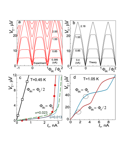
Figure 4: (Color online) SQUTRID characteristics: (a) experimental voltage-flux (signal) characteristics $V_{T}(\Phi_{dc}/\Phi_{0})$ obtained for several amplitudes of rf generator current $I_{0}$ (indicated as the curve parameter) and (b) set of voltage-flux characteristics calculated accounting for noise with standard deviation $\sigma=0.013$ at currents $I_{0}$ close to the experimental values (curve parameter). Independently measured SQUTRID parameters $L_{q}=3\!\times\!10^{-10}$ H, $\beta_{L}=4.0$, $L_{T}=1.2\!\times\!10^{-6}$ H, $M=1.52\!\times\!10^{-9}$ H, $Q=302$, $k^{2}Q=1.89$, and capacitance $C=4.36$ fF were used in the calculations. (c) Experimental (dots) and theoretical voltage-current characteristics $V_{T}(I_{0})$ calculated for noise flux standard deviations $\sigma=0.013$ (dotted line) and $\sigma=0.023$ (dashed line) at $\Phi_{dc}=\Phi_{0}$ and no-superposition experimental (squares) voltage-current characteristic $V_{T}(I_{0})$ at $\Phi_{dc}=\Phi_{0}/2$; (d) smearing of $V_{T}(I_{0})$ curves when the refrigerator temperature rises to $T=1.05$ K. Nonlinearities due to the superposition (circled) almost vanish.

Figure 4(c) presents the initial parts of the SQUTRID $V_{T}(I_{0})$ characteristics ($\beta_{L}\approx 4$) registered for two values of the magnetic flux, $\Phi_{dc}=\Phi_{0}$ and $\Phi_{dc}=\Phi_{0}/2$. The theoretical curves $V_{T}(I_{0})$ are derived from Eqs. (9) with experimentally measured SQUTRID parameters and averaging the superposition nonlinearity of the quantum system over low-frequency noise (10) with standard deviations $\sigma=0.013$ and $\sigma=0.023$. For the V-I curves with $\Phi_{dc}=n\Phi_{0}$, the effective reciprocal quantum inductance of the base superposition qutrit level, introduced into the tank at low rf generator currents ($I_{0}\leq 0.4$ nA), leads to a large shift in the tank resonance frequency from the generator frequency, which results in a decrease in the voltage detected at the $L_{T}C_{T}$ tank down to a value comparable to the noise level. As seen from Eqs. (9) and (10), at $\Phi_{dc}=n\Phi_{0}$ and a low current (linear) regime the voltage reads approximately as $V_{T}\approx\omega_{T}L_{T}I_{0}Q/|k^{2}Q(L_{q}L_{Q}^{-1})_{\!eff}^{\,\min}|$; that is, it is reduced by a factor of $|k^{2}Q(L_{q}L_{Q}^{-1})_{\!eff}^{\,\min}|\gg 1$ compared to the autonomous $L_{T}C_{T}$ tank voltage.

The theoretical curve $V_{T}(I_{0})$ with noise standard deviation $\sigma=0.013$ coincides with the experimental curve in the range of low-to-moderate generator currents. At higher $\sigma$, the factor $|k^{2}Q(L_{q}L_{Q}^{-1})_{\!eff}^{\,\min}|$ decreases, and the slope of the V-I curve in the area of small rf generator currents becomes higher than in experiment [see the curve with $\sigma=0.023$ in Fig. 4(c)]. At $I_{0}>2.5$ nA, the amplitude of ac magnetic flux induced in the SQUTRID loop $\Phi_{ac}=MV_{T}(I_{0})/(\omega_{T}L_{T})$ exceeds the half-width of the “main dip” of the effective reciprocal quantum inductance, $\Phi_{ac}>0.02\Phi_{0}$ [see Fig. 3(d)], and then $V_{T}$ rapidly rises with the increase in the rf generator current. Such behavior at high rf generator currents $I_{0}$ (nonlinear regime) is well described by the proposed theoretical model. The observed quantitative deviation can be attributed to both simplifications made when deriving the theoretical model (ideal ScS contact, zero SQUTRID temperature, and Gaussian noise distribution) and an experimental error in determining the SQUTRID parameters. The no-superposition quasiautonomous-tank experimental V-I curve at $\Phi_{dc}=\Phi_{0}/2$, which is related to the considered “plateau regime” in $V_{T}(\Phi_{dc})$ characteristics, is shown in Fig. 4(c). It is seen that this V-I curve follows Ohm’s law at the specified $\beta_{L}\approx 4$. As discussed above, with a high enough barrier, separating the two wells in the two-well potential, the qutrit wave function remains localized in one of them during the variation of the potential by the ac component of the external magnetic flux.

The impact of thermodynamic fluctuations on the effective reciprocal quantum inductance (10) and on the rf V-I characteristics of the SQUTRID is illustrated in Fig. 4(d). The nonlinearity due to the superposition of states is severely smeared out by temperature at $T=1.05$ K and becomes completely unobservable in our experiments at helium bath temperature $T\geq 1.5$ K. This result can be explained by an increase in the higher-level population because of the reduction of the ratio $\Delta E_{01}/k_{B}T\lesssim 1$ and an essential increase in the noise flux variance $\sigma^{2}$.

To see nonlinearities caused by the superposition of states in more complicated potentials, we have increased the critical current of the SQUTRID ScS contact up to $I_{c}\approx 8\,\mu$A. An increased $I_{c}$ and, thus $\beta_{L}$, parameter corresponds to contacts with a greater number of atoms (atomic rows) at their opening and hence decreased values of their normal-state resistance $R_{N}$. Figure 5(a) displays rf V-I characteristics of the SQUTRID with $\beta_{L}\approx 7.3$ obtained at temperature $T=450$ mK for magnetic fluxes $\Phi_{dc}=n\Phi_{0}$ and $\Phi_{dc}=(n+\!1/2)\,\Phi_{0}$. The initial parts of both branches of the V-I curves remain almost linear due to dynamic localization of the qutrit wave function. The effect of the reciprocal quantum inductance determined by the effective curvature (10) of the base superposition level $E_{S0}$ is observable at generator currents less than those needed to form “classical” steps in SQUID rf V-I characteristics. Figure 5(b) shows superposition energy levels calculated for $\beta_{L}=7.3$ that appear in the four-well symmetrical potential at $\Phi_{e}(t)=1.5\Phi_{0}$. Despite the fact that, at chosen SQUTRID parameters, the environment needs to absorb a considerable amount of energy [$(E_{S0}-E_{-1})/k_{B}\approx 7$ K] when the system relaxes to the lower level, the relaxation events often occurred in the experiment. This can be caused by very high numbers of superposition energy levels ($n=100$ in our case) that are less stable with respect to noise and by possible dissipation effects related to an increase in the number of atoms in the contact. The effect of the energy relaxation resulting in a jump to a linear part of another ($\Phi_{dc}=0$) no-superposition branch of the V-I curve is shown in Fig. 5(a) by the up arrow. The reverse process of the transition from the no-superposition V-I branch to the superposition one shown by the down arrow reflects the formation of the superposition state in the four-well symmetrical potential configuration at a driving current that gives the total external flux $\Phi_{e}(t)=1.5\Phi_{0}$.

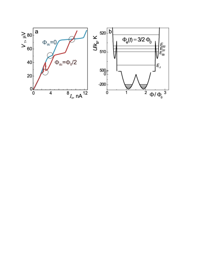
Figure 5: (Color online) Superposition of states in the superconducting ring closed by ScS contact, with a four-well potential. (a) Experimental voltage-current characteristics of the SQUTRID with $\beta_{L}\approx 7.3$ obtained at $T=450$ mK for external magnetic fluxes $\Phi_{dc}=\Phi_{0}/2$ and $\Phi_{dc}=\Phi_{0}$. The areas where the effect associated with maximal local curvature of the base superposition level appears are circled. The jumps shown by the arrows are due to relaxation events. (b) Potential energy and superposition energy levels calculated for the SQUTRID parameters taken from experimental data. Three superposition levels still form in this four-well potential and are situated far above two middle wells.

Note that small amplitudes of the SQUTRID driving current in quantum measurements are the most favorable for quantum informatics. The obtained conversion ratio ($\eta=dV_{T}/d\Phi_{e}\approx 3\!\times\!10^{10}$ V$/$Wb) and the SQUTRID performance in the three-well superposition (at $\beta_{L}\approx 4$) can be further increased by increasing the frequency $\omega$ while simultaneously and proportionally reducing the generator current $I_{0}$. For example, at pumping frequency $\omega/2\pi=100\,$MHz we have $\eta$ of up to $5\times\!10^{11}$ V$/$Wb. In this case the SQUTRID voltage-flux characteristics would be similar to those shown in Figs. 4(a) and 4(b) for small ($I_{0}\leq 0.4$ nA) current amplitudes. Since, as shown in Ref. 16, , the detector and the tank temperature in these measurements may be as low as $10$ mK and the SQUTRID acts as a sensor of parametric quantum inductance under adiabatic conditions, such a device can be considered to be a representative of the class of quantum-limited detectors.

IV Summary and conclusions

We have constructed and studied a new ideal parametric detector of magnetic flux named rf SQUTRID which is based on quantum superposition of three macroscopic flux states of a 3D toroidal superconducting loop closed by Nb-Nb atomic-size point contact. Due to the specific form of the potential barrier, the small contact capacitance, and the fast tunneling dynamics of formation of a coherent three-well superposition state ($\tau_{S}\sim 3\!\times\!10^{-11}$ s), the adiabatic conditions in the rf SQUTRID are valid up to frequencies $\omega/2\pi\approx 3$ GHz for small driving amplitudes ($MI_{0}\sim 10^{-3}\Phi_{0}$). Therefore, the flux detectors based on the dependence of the local curvature of the base superposition energy level (or quantum inductance) on the external magnetic flux at low temperatures fall well within the class of fast and sensitive devices. Note that unlike the rf SQUTRID/SQUBID based on the atomic-size point contact, similar detectors with contacts of the SIS type will have slow tunneling dynamics of flux wave packets and, respectively, a lower operating speed. The rf SQUTRID (as well as rf SQUBID) is the flux magnetometer ”dual” to the rf single electron transistor (SET) electrometer,RF-SET and so the main applications of the rf SQUTRID will initially be experimental study of physical processes in flux qubits and engineering readout systems (sensors) for reading states in the small-scale superconducting quantum registers using weak continuous measurements.

We stress the following results of this paper: (i) The coherent superposition state $\Psi_{S0}(f)$ of wave functions corresponding to three distinct macroscopic states is formed in the three-well symmetrical potential configuration at $\Phi_{e}=n\Phi_{0}$ in the superconducting circuit with the clean atomic-size ScS contact under study. (ii) The energy relaxation time $\tau_{\varepsilon}$ of the base superposition state $\Psi_{S0}(f)$ to lower energy states can be macroscopically large to perform quantum measurements. (iii) Unlike classical rf SQUID in a nonhysteretic regime, the nonlinear properties of the superposition in the three-well potential under the condition $\omega/2\pi\ll\nu_{01}\ll\Delta_{0}/h$ enable making a sensitive and fast parametric detector of magnetic flux without a quasiparticle current, i.e., principally a nondissipative rf SQUTRID device. (iv) An unusually large splitting $\Delta E_{01}/k_{B}=1.5-2$ K and a very large (at low noise variance) $L_{q}L_{Q}^{-1}\approx 200$, specifying the nonlinearity of the studied quantum system, make the rf SQUTRID with a ScS contact a very promising element for quantum informatics.

- (1) A.O. Caldeira and A.J. Leggett, Influence of dissipation on quantum tunneling in macroscopic system, Phys. Rev. Lett. 46, 211-214 (1981).
- (2) S. Chakravarty, Quantum fluctuations in the tunneling between superconductors, Phys. Rev. Lett. 49, 681 684 (1982).
- (3) U. Weiss, H. Grabert, S. Linkwitz, Influence of friction and temperature on coherent quantum tunnelling, J. Low Temp. Phys. 68, 213-244 (1987).
- (4) J.R. Friedman, V. Patel, W. Chen, S.K. Tolpygo, J.E. Lukens, Quantum superpositions of distinct macroscopic states, Nature 406, 43-46 (2000).
- (5) C.H. van der Wal, A.C.J. ter Haar, F.K. Wilhelm, R.N. Schouten, C.J.P.M. Harmans, T.P. Orlando, S. Lloyd, J.E. Mooij, Quantum superpositions of macroscopic persistent-current states, Science 290, 773-776 (2000).
- (6) J. Clarke and F.K. Wilhelm, Superconducting quantum bits, Nature 453, 1031-1042 (2008).
- (7) V.I. Shnyrkov, A.A. Soroka, A. M. Korolev, O.G. Turutanov, Superposition of states in flux qubits with Josephson junction of ScS type, Low Temp. Phys. 38 (4), 301-310 (2012).
- (8) V.I. Shnyrkov and S.I. Melnik, Quantum detector based on a superposition of macroscopic states of phase qubit, Low Temp. Phys. 33, 15-22 (2007).
- (9) R. Bianchetti, S. Filipp, M. Baur, J.M. Fink, C. Lang, L. Steffen, M. Boissonneault, A. Blais, A. Wallraff, Control and tomography of a three level superconducting artificial atom, Phys. Rev. Lett. 105, 223601 (2010).
- (10) N. Agraït, A.L. Yeyati, J.M. van Ruitenbeek, Quantum properties of atomic-sized conductors, Phys. Rep. 377 81 279 (2003).
- (11) I.O. Kulik and A.N. Omelyanchouk, Josephson effect in superconducting bridges: microscopic theory, Sov. J. Low Temp. Phys. 4, 142 (1978).
- (12) C.W.J. Beenakker and H. van Houten, Josephson current through a superconducting quantum point contact shorter than the coherence length, Phys. Rev. Lett. 66, 3056 (1991); C.W.J. Beenakker and H. van Houten, The superconducting quantum point contact, arXiv:cond-mat/0512610v1.
- (13) A. Gumann, T. Dahm, N. Schopohl, Microscopic theory of superconductor-constriction-superconductor Josephson junctions in a magnetic field, Phys. Rev. B 76, 064529 (2007).
- (14) I.M. Dmitrenko, V.A. Khlus, G.M. Tsoi, V.I. Shnyrkov, Macroscopic quantum tunnelling in the r.f. SQUID with S-c-S point contacts, Il Nuovo Cimento D9, 1057-1060 (1987).
- (15) I.M. Dmitrenko, V.A. Khlus, G.M. Tsoi, V.I. Shnyrkov, Quantum decay of metastable current states in RF SQUIDs, Sov. J. Low Temp. Phys. 11, 77 (1985).
- (16) A.J. Leggett, Testing the limits of quantum mechanics: motivation, state of play, prospects, J. Phys.: Condens. Matter 14, R415- R451 (2002).
- (17) A.A. Clerk, M. H. Devoret, S.M. Girvin, Florian Marquardt, R.J. Schoelkopf, Introduction to quantum noise, measurement, and amplification, Rev. Mod. Phys. 82, 1155 (2010).
- (18) A.N. Korotkov and D.V. Averin, Continuous weak measurement of quantum coherent oscillations, Phys. Rev. B 64, 165310 (2001).
- (19) A. Yu. Smirnov, Theory of weak continuous measurements in a strongly driven quantum bit, Phys. Rev. B 68, 134514 (2003).
- (20) T.D. Clark, J. Diggins, J.F. Ralph, M. Everitt, R.J. Prance, H. Prance, R. Whiteman, A. Widom, Y.N. Srivastava, Coherent evolution and quantum transitions in a two level model of a SQUID ring, Ann. Phys. 268, 1 (1998).
- (21) Ya.S. Greenberg, A. Izmalkov, M. Grajcar, E. Il ichev, W. Krech, H.-G. Meyer, M.H.S. Amin, A.M. van den Brink, Low-frequency characterization of quantum tunneling in flux qubits, Phys. Rev. B 66, 214525 (2002).
- (22) A.B. Zorin, Josephson charge-phase qubit with radio frequency readout: coupling and decoherence, JETP 98, 1250 (2004).
- (23) M. Grajcar, A. Izmalkov, E. Il ichev, Th. Wagner, N. Oukhanski, U. Hubner, T. May, I. Zhilyaev, H.E. Hoenig, Ya.S. Greenberg, V.I. Shnyrkov, D. Born, W. Krech, H.-G. Meyer, A.M. van den Brink, M.H.S. Amin, Low-frequency measurement of the tunneling amplitude in a flux qubit, Phys. Rev. B 69, 060501(R) (2004).
- (24) E. Il ichev, A.Yu. Smirnov, M. Grajcar, A. Izmalkov, D. Born, N. Oukhanski, Th. Wagner, W. Krech, H.-G. Meyer, A.Zagoskin, Radio-frequency method for investigation of quantum properties of superconducting circuits, Low Temp. Phys. 30, 620 (2004).
- (25) V.I. Shnyrkov, Th. Wagner, D. Born, S.N. Shevchenko, W. Krech, A.N. Omelyanchouk, E. Il’ichev, H.-G. Meyer, Multiphoton transitions between energy levels in a phase-biased Cooper-pair box, Phys. Rev. B 73, 024506 (2006).
- (26) A.H. Nayfeh, Perturbation Methods (Wiley, New York, 1973), p. 165.
- (27) E.M. Lifshitz and L.D. Landau, Statistical Physics: Course of Theoretical Physics, 3rd ed., Vol. 5, Chap. 12, p. 359 (Butterworth, London, 1984).
- (28) A.M. Korolev, V.I. Shnyrkov, V.M. Shulga, Ultra-high frequency ultra-low dc power consumption HEMT amplifier for quantum measurements in millikelvin temperature range, Rev. Sci. Instrum. 82, 016101 (2011).
- (29) R.J. Schoelkopf, P. Wahlgren, A.A. Kozhevnikov, P. Delsing, D.E. Prober, The radio-frequency single-electron transistor (RF-SET): a fast and ultrasensitive electrometer, Science 280, 1238 (1998).