On the Minimum Differential Feedback for Time-Correlated MIMO Rayleigh Block-Fading Channels

Abstract

In this paper, we consider a general multiple input multiple output (MIMO) system with channel state information (CSI) feedback over time-correlated Rayleigh block-fading channels. Specifically, we first derive the closed-form expression of the minimum differential feedback rate to achieve the maximum erdodic capacity in the presence of channel estimation errors and quantization distortion at the receiver. With the feedback-channel transmission rate constraint, in the periodic feedback system, we further investigate the relationship of the ergodic capacity and the differential feedback interval, and we find by theoretical analysis that there exists an optimal differential feedback interval to maximize ergodic capacity. Finally, analytical results are verified through simulations in a practical periodic differential feedback system using Lloyd’s quantization algorithm.

I Introduction

Channel state information (CSI) feedback from the receiver to the transmitter has been intensively studied with great interest due to its potential benefits to the multiple input multiple output (MIMO) system. CSI can be utilized by a variety of channel adaptive techniques (e.g., water-filling, beamforming, precoding, etc.) at the transmitter to enhance the spectral efficiency as well as the robustness of the system, especially, in the frequency division duplexing (FDD) mode. As the transmission rate of the feedback channel is normally very limited, the infinite feedback of CSI is hard to realize in practice. Therefore, it is important to investigate how to decrease the amount of feedback signalling overhead to meet the uplink feedback channel requirements. As a result, CSI feedback reduction has attracted lots of attention in recent years [1], [2].

Specifically, when the wireless channel experiences time-correlated fading [3], typically represented by a Markov random process [4]–[6], the amount of CSI feedback can be largely reduced. In [8], a number of feedback reduction schemes were summarized, considering the lossy compression scheme exploiting the properties of fading process as the best choice. In [7] and [9], schemes using switched codebook and rotation codebook with differential feedback were proposed, respectively. In [10], it modeled the time-correlated fading channel as a finite-state Markov chain to reduce the feedback rate by ignoring some states occurred with small probabilities. In [11] and [12], a predictive vector quantization scheme was proposed, provided that the previous quantization CSI is known. In [13], variable-length code was applied for feedback rate reduction. Despite of so much research on practical feedback reduction schemes, the lower bound of the feedback compression as well as the required minimum differential feedback rate to guarantee the accuracy of CSI has not yet been well studied for time-correlated MIMO Rayleigh block-fading channels.

In [14]–[17], the relationship between the capacity gain and the limited feedback of CSI was studied. Lower and upper bounds of ergodic capacity gain using CSI feedback in comparison with open-loop systems were reported in [18] and [19]. However, the time correlation was not taken into account in these work. In [20], a periodic feedback scheme was studied with time correlation, but the feedback only occurs in the first block of the transmission period. Unlike previous work, in this paper, we investigate the relationship between the ergodic capacity and the differential feedback interval with feedback channel capacity constraint in every fading block.

In this paper, we consider a general MIMO system with periodic differential CSI feedback over time-correlated Rayleigh block-fading channels, and address the problem of the ergodic capacity under the impact of the feedback interval. The main contribution can be briefly summarized as follows:

1. We derive the minimum differential feedback rate for time-correlated MIMO Rayleigh block-fading channels by taking into account of both the channel estimation errors and channel quantization distortion.

2. We investigate the relationship between the ergodic capacity and the differential feedback interval with feedback channel rate constraint in a periodic feedback system. Furthermore, we prove that there exists an optimal feedback interval to achieve the maximum ergodic capacity.

3. We design a practical differential feedback scheme using Lloyd’s quantization algorithm to verify the theoretical results.

The rest of the paper is organized as follows. In Section II, we describe the system model. In Section III, the minimum differential feedback rate is derived, and the relationship between the ergodic capacity and differential feedback interval is studied. In Section IV, we provide the simulation results. In Section V, we draw the main conclusions. The derivations are given in the appendices.

Notation: Bold uppercase (lowercase) letters denote matrices (vectors), ${(\cdot)^{+}}$ denotes Hermitian transpose, $\log_{2}(\cdot)$ denotes the base two logarithm, $\det(\cdot)$ denotes determinant operator, and $\mathbb{E}[\cdot]$ stands for the expectation over random variables.

II System Model

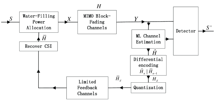
Figure 1: System Model.

The system model is illustrated in Fig. 1, where the downlink channel is modeled as a time-correlated MIMO Rayleigh block-fading channels, and the uplink channel is modeled as a limited and lossless feedback channel with a feedback capacity constraint per fading block. In this paper, we consider the differential feedback, i.e., the receiver just feeds back the differential CSI to the transmitter given the previous channel quantization matrix, where the channel estimation errors and channel quantization distortion are also considered.

II-A Time-Correlated MIMO Rayleigh Block-Fading Channel Model

We consider MIMO Rayleigh block fading channels, where the channel fading matrix remains constant within a fading block and varies from one to another. There are $N_{t}$ transmitter antennas and $N_{r}$ receiver antennas. The received signals can be expressed in a vector form

$$\mathbf{y}=\mathbf{Hx}+{\mathbf{n}_{0}},$$ (1)

where ${\bf{y}}={[{y_{1}},{y_{2}},{y_{3}},\ldots,{y_{{N_{r}}}}]^{T}}$ denotes a ${N_{r}}\times 1$ received signal vector, $\mathbf{H}$ is a ${N_{r}}\times{N_{t}}$ channel fading matrix with independent entries obeying complex Gaussian distribution $\mathcal{C}\mathcal{N}(0,\sigma_{h}^{2})$, ${\bf{x}}={[{x_{1}},{x_{2}},{x_{3}},\ldots,{x_{{N_{t}}}}]^{T}}$ represents a ${N_{t}}\times 1$ transmitted signal vector, and $\mathbf{n}_{0}$ is a ${N_{r}}\times 1$ noise vector whose entries are independent and identically distributed (i.i.d) complex Gaussian variables $\mathcal{C}\mathcal{N}(0,\sigma_{0}^{2})$.

The time-correlated channel can be represented by a first-order Autoregressive model (AR1) [6], and the channel fading matrix can be written as

$${\mathbf{H}_{n}}=\alpha{\mathbf{H}_{n-1}}+\sqrt{1-{\alpha^{2}}}{\mathbf{W}_{n}},$$ (2)

where ${\mathbf{H}_{n-1}}$ denotes ${(n-1)_{th}}$ channel fading matrix, $\mathbf{W}_{n}$ is a noise matrix, which is independent of ${\mathbf{H}_{n-1}}$, and the entries are i.i.d. complex Gaussian variables $\mathcal{C}\mathcal{N}(0,\sigma_{h}^{2})$. The parameter $\alpha$ is the time autocorrelation coefficient, which is given by the zero-order Bessel function of first kind $\alpha={J_{0}}(2\pi{f_{d}}\tau)$ [6], where $f_{d}$ denotes the maximum Doppler frequency in Hertz, and $\tau$ denotes the time interval. In the block-fading system, the time interval can be calculated as $T=\tau/{t_{block}}$, where $t_{block}$ is the duration of every block.

The CSI can be estimated by the receiver using orthogonal pilots. Without loss of generality, in this paper, maximum likelihood (ML) criterion is employed for channel estimation, and the estimated channel matrix can be expressed in an equivalent form as

$$\hat{\mathbf{H}}=\mathbf{H}+\mathbf{H}_{e},$$ (3)

where $\hat{\mathbf{H}}$ denotes the channel estimation matrix, whose entries are i.i.d. complex Gaussian variables $\mathcal{C}\mathcal{N}(0,\sigma_{\hat{h}}^{2})$, $\mathbf{H}$ is the actual channel fading matrix, and $\bf{H}_{e}$ denotes the channel estimation error matrix, which is independent of $\mathbf{H}$, with entries of independent complex Gaussian distributed with $\mathcal{C}\mathcal{N}(0,\sigma_{\hat{h}}^{2}-\sigma_{h}^{2})$ [21].

As $\mathbf{H}_{e}$ is independent of $\mathbf{H}$ in (3), we obtain

$${\mathbf{H}}=\frac{{\sigma_{h}^{2}}}{{\sigma_{\hat{h}}^{2}}}\hat{\mathbf{H}}+\bf{\Psi},$$ (4)

where $\sigma_{h}^{2}$ and $\sigma_{\hat{h}}^{2}$ denote the variances of $\mathbf{H}$ and $\hat{\mathbf{H}}$, respectively, and $\bf{\Psi}$ is independent of $\hat{\mathbf{H}}$ with entries satisfying $\mathcal{C}\mathcal{N}\left({0,\frac{{\sigma_{h}^{2}\cdot(\sigma_{\hat{h}}^{2}-\sigma_{h}^{2})}}{{\sigma_{\hat{h}}^{2}}}}\right)$. The detailed derivation of (4) is given in Appendix A.

II-B CSI Feedback Model

We consider a limited and lossless feedback channel. Through CSI quantization, the feedback channel output $\bar{\mathbf{H}}$ can be modeled as [18]

$$\hat{\mathbf{H}}=\bar{\mathbf{H}}+\mathbf{E},$$ (5)

where $\mathbf{E}$ denotes the independent additive quantization error matrix with entries satisfying $\mathcal{C}\mathcal{N}\left({0,\frac{D}{{{N_{r}}{N_{t}}}}}\right)$, where $D$ represents the channel quantization distortion constraint.

In this paper, we consider the differential feedback, where only the differential CSI will be fed back to the transmitter, assuming that the previous channel quantization matrix ${\bar{\mathbf{H}}_{n-1}}$ is known both at receiver and transmitter. The differential CSI can be written as

$${\mathbf{H}_{d}}=Diff\left({\hat{\mathbf{H}}_{n},{{\bar{\mathbf{H}}}_{n-1}}}\right),$$ (6)

where ${\mathbf{H}_{d}}$ represents the differential CSI between $\hat{\mathbf{H}}_{n}$ and ${\bar{\mathbf{H}}_{n-1}}$, and $Diff(\cdot)$ denotes the differential function.

Furthermore, we assume that the CSI feedback channel has a capacity constraint ${C_{fb}}$ per fading block. When the CSI is quantized to $R$ bits and the feedback interval is $T$ blocks, the average feedback rate satisfies the inequality $R/T\leq{C_{fb}}$. Therefore, the feedback interval can be calculated by

$$T=\left\lceil{\frac{R}{{{C_{fb}}}}}\right\rceil,$$ (7)

where $\left\lceil x\right\rceil$ denotes the smallest integer larger than $x$.

II-C Ergodic Capacity of Pilot-assisted MIMO Systems

In this paper, we use the water-filling precoder to obtain the capacity gain. The channel quantization matrix can be decomposed at the transmitter to perform water-filling ??????water-filling reference??????

$$\bar{\mathbf{H}}=\mathbf{U}\bf{\Sigma}{\mathbf{V}^{+}},$$ (8)

where $\mathbf{U}$ and $\mathbf{V}$ are unitary matrixes, and $\bf{\Sigma}$ is a non-negative and diagonal matrix composed of eigenvalues.

For the pilot-assisted MIMO system with ML channel estimation, the closed-loop ergodic capacity with water-filling can be obtained with the help of [20, 21]

$${C_{erg}}=\mathbb{E}_{\hat{\mathbf{H}},\bar{\mathbf{H}}}\left[{\frac{{L-{N_{t}}}}{L}{{\log}_{2}}\det\left({{\mathbf{I}_{{N_{r}}}}+\mathbf{J}\cdot{\mathbf{J}^{+}}\left({{\mathbf{F}^{-1}}}\right)}\right)}\right],$$ (9)

where $\mathbf{J}=\hat{\mathbf{H}}\mathbf{V}\mathbf{Z}$, ${\mathbf{J}_{e}}={\mathbf{H}_{e}}\mathbf{V}\mathbf{Z}$, $\mathbf{F}=\frac{1}{A^{2}}{\mathbf{I}_{{N_{r}}}}+{E_{{\mathbf{J}_{e}}}}\left[{{\mathbf{J}_{e}}\mathbf{J}_{e}^{+}|\mathbf{J}}\right]$, $L$ denotes the number of transmitted symbols, $A$ represents the amplitude of signal symbol, and $\mathbf{Z}$ stands for a diagonal matrix determined by the water-filling algorithm, which is given by ??????reference??????

$$\left\{\begin{array}[]{l}z_{{}_{i}}^{2}=\left\{\begin{array}[]{l}\mu-{\left({\gamma_{i,i}^{2}{A^{2}}}\right)^{-1}},\;\gamma_{i,i}^{2}{A^{2}}\geq{\mu^{-1}}\\ 0,\quad\quad\quad\quad\quad\;otherwise\\ \end{array}\right.\\ \sum\limits_{i=1}^{{N_{t}}}{z_{{}_{i}}^{2}{A^{2}}={N_{t}}{A^{2}},}\\ \end{array}\right.$$ (10)

where ${\gamma_{i,i}}$ are entries of $\mathbf{\Sigma}$, and $\mu$ is a cut-off value chosen to meet the power constraint.

It can be observed from (9) that the closed-loop ergodic capacity is determined by $\bar{\mathbf{H}}$ and $\hat{\mathbf{H}}$, and the loss of the capacity is mainly caused by the distortion. Hence, the ergodic capacity is a negative-correlated function in association with the distortion of CSI feedback [14, 17].

III Minimum Differential Feedback Rate

In this section, we derive the minimum differential feedback rate of the time-correlated MIMO Rayleigh block-fading channels to guarantee the accuracy of the CSI. The minimum differential feedback rate is determined by the rate distortion theory of continuous-amplitude sources ??????reference??????. When the ${(n-1)_{th}}$ channel quantization matrix ${\bar{\mathbf{H}}_{n-1}}$ is known at both receiver and transmitter, the minimum differential feedback rate can be written as

$$R=\inf\left\{{I\left({{{\hat{\mathbf{H}}}_{n}};{{\bar{\mathbf{H}}}_{n}}|{{\bar{\mathbf{H}}}_{n-1}}}\right):E\left[{d\left({{{\hat{\mathbf{H}}}_{n}};{{\bar{\mathbf{H}}}_{n}}}\right)}\right]\leq D}\right\},$$ (11)

where $\inf\left\{\cdot\right\}$ denotes infimum function [23], ${I\left({{{\hat{\mathbf{H}}}_{n}};{{\overline{\mathbf{H}}}_{n}}|{{\overline{\mathbf{H}}}_{n-1}}}\right)}$ denotes the mutual information between $\hat{\mathbf{H}}_{n}$ and $\bar{\mathbf{H}}_{n}$ given $\bar{\mathbf{H}}_{n-1}$, and $d\left({{{\hat{\mathbf{H}}}_{n}},{{\bar{\mathbf{H}}}_{n}}}\right)={\left\|{{{\hat{\mathbf{H}}}_{n}}-{{\bar{\mathbf{H}}}_{n}}}\right\|^{2}}$ is the channel quantization distortion, which is the measurement of the quality of feedback information.

Since the entries of $\mathbf{H}$, $\hat{\mathbf{H}}$ and $\bar{\mathbf{H}}$ are i.i.d. complex Gaussian variables, the minimum differential feedback rate can be written as

$$R=\inf\left\{{{N_{r}}{N_{t}}\cdot I\left({{{\hat{h}}_{n}};{{\bar{h}}_{n}}|{{\bar{h}}_{n-1}}}\right):E\left[{d\left({{{\hat{h}}_{n}};{{\bar{h}}_{n}}}\right)}\right]\leq d}\right\},$$ (12)

where $d=\frac{D}{{{N_{r}}{N_{t}}}}$ denotes the one-dimensional average channel quantization distortion, and ${\hat{h}_{n}}$, ${\bar{h}_{n}}$, and ${\bar{h}_{n-1}}$ denote the entries of ${\hat{\mathbf{H}}_{n}}$, ${\bar{\mathbf{H}}_{n}}$, and ${\bar{\mathbf{H}}_{n-1}}$, respectively.

Lemma 1

Given the one-dimensional channel quantization distortion constraint $d$, and the ${\left({n-1}\right)_{th}}$ channel quantization element ${\bar{h}_{n-1}}$, the mutual information $I\left({{{\hat{h}}_{n}};{{\bar{h}}_{n}}|{{\bar{h}}_{n-1}}}\right)$ can be calculated as

$$I\geq\log\left[{{\alpha^{2}}{{\left({\frac{{\sigma_{h}^{2}}}{{\sigma_{\hat{h}}^{2}}}}\right)}^{2}}+\frac{{\left({1-{\alpha^{2}}}\right)}}{d}\sigma_{h}^{2}+\frac{{\left({\sigma_{\hat{h}}^{2}-\sigma_{h}^{2}}\right)}}{d}}\right.\left.{\left({1+{\alpha^{2}}\frac{{\sigma_{h}^{2}}}{{\sigma_{\hat{h}}^{2}}}}\right)}\right],$$ (13)

where $\sigma_{h}^{2}$ and $\sigma_{\hat{h}}^{2}$ denote the variances of $h$ and $\hat{h}$ respectively, and $\alpha$ is the time autocorrelation coefficient.

The proof of Lemma 1 can be found in Appendix B. As ${\hat{h}_{n}}$, ${\bar{h}_{n}}$ and ${\bar{h}_{n-1}}$ are complex Gaussian variables, the minimum value of the mutual information is indeed achievable [23].

Combining (12) and (13), the minimum differential feedback rate of the time-correlated MIMO block-fading channels can be calculated as

$$R={N_{r}}{N_{t}}\cdot\max\left\{{\log\left[{{\alpha^{2}}{{\left({\frac{{\sigma_{h}^{2}}}{{\sigma_{\hat{h}}^{2}}}}\right)}^{2}}+\frac{{\left({1-{\alpha^{2}}}\right)}}{d}\sigma_{h}^{2}}\right.}\right.\left.{\left.{+\frac{{\left({\sigma_{\hat{h}}^{2}-\sigma_{h}^{2}}\right)}}{d}\left({1+{\alpha^{2}}\frac{{\sigma_{h}^{2}}}{{\sigma_{\hat{h}}^{2}}}}\right)}\right],0}\right\}.$$ (14)

From (14), we can see that the minimum differential feedback rate is determined by the distortion of the quantization, time correlation coefficient, and the estimation variance. Note that the minimum differential feedback rate in (14) is the lower bound of feedback compression with time correlation in the block-fading MIMO channels. Given the accuracy of feedback CSI (i.e. the distortion $d$), the minimum feedback rate can be easily obtained in (14).

Furthermore, as the ergodic capacity increases with the distortion decreasing, we investigate the feedback design scheme for minimizing the distortion of the feedback CSI in order to maximize the ergodic capacity in the following.

From (14), if $R\geq 0$, $d$ can be calculated as

$$d=\left({\sigma_{\hat{h}}^{2}-{{\left({\frac{{\sigma_{h}^{2}}}{{\sigma_{\hat{h}}^{2}}}}\right)}^{2}}\sigma_{\hat{h}}^{2}\cdot{\alpha^{2}}}\right)/\left({{2^{\frac{R}{{{N_{r}}{N_{t}}}}}}-{\alpha^{2}}{{\left({\frac{{\sigma_{h}^{2}}}{{\sigma_{\hat{h}}^{2}}}}\right)}^{2}}}\right).$$ (15)

In a practical communication system, the feedback channel is causal, which implies that ${\bar{\mathbf{H}}_{n}}$ can be only used in the next feedback period ${{{\hat{\mathbf{H}}}_{n+1}}}$. With the causal feedback constraint, we consider the impact of the feedback delay on the distortion. Combining (15) and (35), the distortion can be written as

$$d={\alpha^{2}}{\left({\frac{{\sigma_{h}^{2}}}{{\sigma_{\hat{h}}^{2}}}}\right)^{2}}\frac{{\sigma_{\hat{h}}^{2}-{{\left({\frac{{\sigma_{h}^{2}}}{{\sigma_{\hat{h}}^{2}}}}\right)}^{2}}\sigma_{\hat{h}}^{2}\cdot{\alpha^{2}}}}{{{2^{\frac{R}{{{N_{r}}{N_{t}}}}}}-{\alpha^{2}}{{\left({\frac{{\sigma_{h}^{2}}}{{\sigma_{\hat{h}}^{2}}}}\right)}^{2}}}}+{\alpha^{2}}\frac{{\sigma_{h}^{2}\left({\sigma_{\hat{h}}^{2}-\sigma_{h}^{2}}\right)}}{{\sigma_{\hat{h}}^{2}}}+\left({1-{\alpha^{2}}}\right)\sigma_{h}^{2}+\left({\sigma_{\hat{h}}^{2}-\sigma_{h}^{2}}\right).$$ (16)

Given $\sigma_{h}^{2}$ and $\sigma_{\hat{h}}^{2}$, we can see that $d$ is a function of $R$ and $\alpha$ in (16). In a periodic feedback system with limited feedback, indicated by (2) and (7), both $\alpha$ and $R$ are related to $T$. Therefore, after some manipulations, the distortion $d$ can be expressed as a function of $T$,

$$d\left(T\right)=\frac{{\sigma_{h}^{4}}}{{\sigma_{\hat{h}}^{2}}}\cdot\left({\frac{{\left({1-{2^{\frac{{{C_{fb}}T}}{{{N_{r}}{N_{t}}}}}}}\right)\alpha{{\left(T\right)}^{2}}}}{{{2^{\frac{{{C_{fb}}T}}{{{N_{r}}{N_{t}}}}}}-{{\left({\frac{{\sigma_{h}^{2}}}{{\sigma_{\hat{h}}^{2}}}}\right)}^{2}}\alpha{{\left(T\right)}^{2}}}}}\right)+\sigma_{\hat{h}}^{2}.$$ (17)

From (17), we have

$$T\to 0\qquad\Rightarrow\quad\quad{2^{\frac{{{C_{fb}}T}}{{{N_{r}}{N_{t}}}}}}\to 1\qquad\Rightarrow\quad d\to\sigma_{\hat{h}}^{2}.$$ (18)

Similarly, when $T$ is large enough, the time correlation $\alpha\left(T\right)$ trends to $0$. Therefore, we have

$$T\to\infty\qquad\Rightarrow\quad\alpha(T)\to 0\qquad\Rightarrow\quad d\to\sigma_{\hat{h}}^{2}.$$ (19)

There are some interesting observations from (18) and (19): When $T$ trends to zero, the channel state remains static, such that it is not necessary to send any feedback bits. Therefore, the quantization channel at the transmitter is independent of the estimation channels at receiver. On the other hand, if $T$ is large enough, the time correlation decreases to zero, which implies that the feedback quantization channel is completely outdated and it is also independent of the estimation channel. Therefore, the distortion in both (18) and (19) are $\sigma_{\hat{h}}^{2}$.

When $0<T<\infty$, we have $0<{\alpha}\left(T\right)^{2}<1$ and $1<{2^{\frac{{{C_{fb}}T}}{{{N_{r}}{N_{t}}}}}}$. Hence, we can obtain that the first term of (17) is negative, and

$$0<T<\infty\qquad\Rightarrow\qquad d<\sigma_{\hat{h}}^{2}.$$ (20)

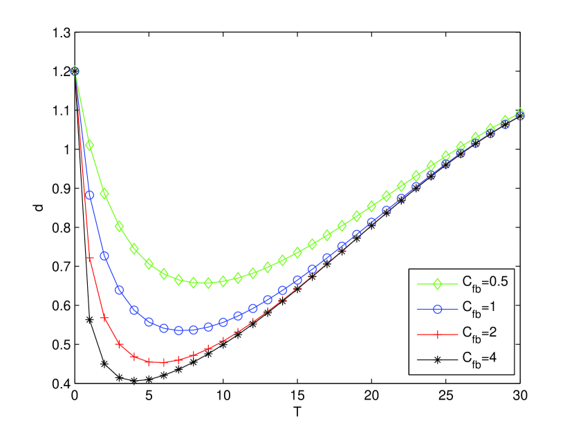
Figure 2: The relationship between the distortion of channel state information feedback and the feedback interval for $N_{r}=2$, $N_{t}=2$, ${\sigma_{h}^{2}}=1$ and ${\sigma_{\hat{h}}^{2}}=1.2$.

Combining (18), (19) and (20), we can predict that there exists an optimal $T$ in the region $(0,\infty)$ to minimize the distortion. We give the proof of the existence of the optimal feedback interval $T$ in the Appendix C. To further verify the theoretical analysis, numerical results of the relationship between the distortion and the feedback interval from (17) are given in Fig. 2.

IV Simulation Results and Discussion

In this section, we first provide the simulation results for the derived minimum differential feedback rate expression. Then, we discuss the relations between the ergodic capacity andthe feedback interval in a periodic feedback system with feedback channel transmission rate constraint. Finally, we verify our theoretical results by a practical differential feedback system employing Lloyd’s quantization algorithm. All simulations are performed for a point-to-point MIMO system over time-correlated block fading channels. For simplicity and without loss of generality, we consider ${N_{t}}=2$ antennas at transmitter, ${N_{r}}=2$ antennas at receiver, and the channel variance is set as $\sigma_{h}^{2}=1$.

IV-A Minimum Differential Feedback Rate

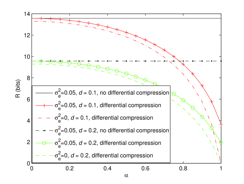
Figure 3: The relationship between the minimum differential feedback rate and time correlation for $N_{r}=2$, $N_{t}=2$, $\sigma_{e}^{2}=\left\{{0,0.05}\right\}$ and $d=\{0.1,0.2\}$.

Fig. 3 shows that the minimum differential feedback rate versus the time correlation with the variance of channel estimation error $\sigma_{e}^{2}=\sigma_{\hat{h}}^{2}-\sigma_{h}^{2}=\left\{{0,0.05}\right\}$, and the accuracy of CSI is represented by the distortion with $d=\{0.1,0.2\}$. We also include the non-differential compression results for comparison.

In Fig. 3, we can see that when time correlation increases, it results in significant reduction of feedback rate by using differential compression. In addition, the impact of estimation error and quantization distortion is also illustrated in Fig. 3. For lower quantization distortion, larger minimum feedback rate is required. It can be also observed from Fig. 3 that with more estimation errors, the feedback rate has to be increased.

IV-B Ergodic Capacity and Feedback Interval

In this subsection, we give the simulation results of the relationship between the ergodic capacity and the feedback intervals. For simplicity, we assume that the block size is $L=100$ with the duration of $1$ ms, and the power of pilot is $10\%$ of the total transmit power, which is a reasonable value in practice [21]. We select a relatively smaller value of SNR, which is $0$ dB, and the Doppler frequency is $9.26$ Hz (Moving speed is $5$ km/h, and the Carrier Frequency is $2$ GHz).

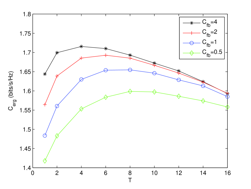
Figure 4: The relationship between the ergodic capacity and feedback interval for ${N_{r}}=2,{N_{t}}=2$, $SNR=0dB$, $L=100$ and ${f_{D}}=9.26$ Hz.

In Fig. 4, we plot the relations between ergodic capacity and the feedback interval with the feedback capacity constraint $C_{fb}=\{0.5,1,2,4\}$ for every block. It clearly shows that the ergodic capacity is a monotonic convex function of the feedback interval, and there exists an optimal feedback interval which maximizes the ergodic capacity. The results are reasonable, because when $T$ increases from a small region, it begins to provide larger feedback rate and thus improve the quality of feedback information, while when $T$ goes toward a relatively larger region, the time correlation gradually decreases and the feedback delay becomes larger, causing the feedback information outdated and therefore impair the performance.

Note that the relations between $C_{erg}$ and $T$ in Fig. 4 is consistent with the analysis in section III, and the similar optimal values of $T$ can be also found in Fig. 2. Additionally, from Fig. 4, we can see that as ${C_{fb}}$ increases, the ergodic capacity also enhances. However, the absolute increment becomes smaller, which implies that it is necessary to limit the feedback channel transmission rate since little gain can be achieved when ${C_{fb}}$ becomes very large.

IV-C Differential Feedback System with Lloyd’s Quantization Algorithm

In order to verify our theoretical results, we design a differential feedback system using Lloyd’s quantization algorithm [24]. Firstly, differential codebooks are generated by Lloyd’s quantization algorithm and available at both receiver and transmitter. When the ${\left({n-1}\right)_{th}}$ channel quantization matrix ${\bar{\mathbf{H}}_{n-1}}$ is known both at receiver and transmitter, the receiver only feeds back the differential codeword to the transmitter.

The feedback steps are given as follows. Firstly, the receiver calculates true quantization error ${\mathbf{H}_{d}}={\hat{\mathbf{H}}_{n}}-{\bar{\mathbf{H}}_{n-1}}$. Secondly, this true error is quantized as ${\mathbf{C}_{d}}$ in the differential codebooks with the smallest Euclidean distance to the true error. Thirdly, the corresponding codeword index is sent back to the transmitter. Finally, the transmitter recovers the channel quantization matrix by ${\bar{\mathbf{H}}_{n}}={\bar{\mathbf{H}}_{n-1}}+{\mathbf{C}_{d}}$.

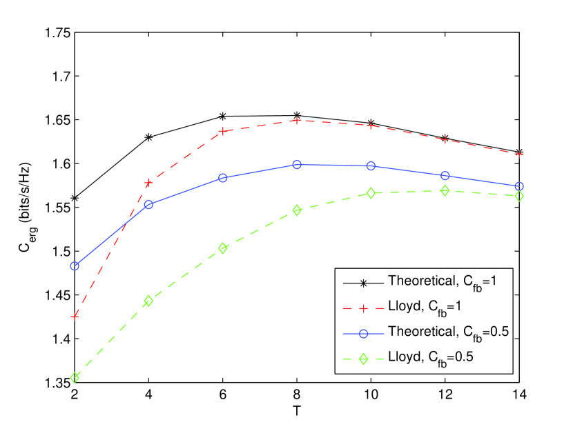
Figure 5: The relationship between the ergodic capacity and feedback interval with Lloyd algorithm for ${N_{r}}=2,{N_{t}}=2$, $SNR=0dB$, $L=100$ and ${f_{D}}=9.26$ Hz.

Fig. 5 shows the ergodic capacity using the Lloyd’s quantization algorithm (dash curves) have the same trend with theoretical ones (solid curves) and there exists an optimal feedback interval. From Fig. 5, it shows that the ergodic capacity of theoretical results is larger than the practical ones at small feedback interval region, but they get converged as the feedback interval increases. The reasons are given as follows. When the feedback interval is in the small region, the feedback rate is not sufficient both for theoretical and practical results, since the codebooks generated with Lloyd’s quantization algorithm have stronger randomization. However, when the feedback rate is small, with the increase of the feedback interval, the more feedback rate can be obtained, reducing the randomization of Lloyd’s quantization algorithm and thus, making the performance converged to the theoretical results.

V Conclusions

In this paper, we have derived the minimum differential feedback rate for the time-correlated Rayleigh block-fading channels considering channel estimation error and quantization distortion. We found that the minimum differential feedback rate is the lower bound of feedback compression with time correlation. We also investigated the relationship between the ergodic capacity and the feedback interval provided the feedback-channel constraint ${C_{fb}}$ per fading block. We found that the ergodic capacity is a monotonic convex function on feedback intervals, and there exists an optimal feedback interval to maximum the ergodic capacity. The simulation results of a practical differential feedback with Lloyd’s quantization algorithm is provided to validate our theoretical results.

Appendix A: Proof of (4)

Substituting (3) into (4), it yields

$$\bf{\Psi}=\left({1-\frac{{\sigma_{h}^{2}}}{{\sigma_{\hat{h}}^{2}}}}\right)\mathbf{H}-\frac{{\sigma_{h}^{2}}}{{\sigma_{\hat{h}}^{2}}}{\mathbf{H}_{e}},$$ (21)

where $\sigma_{h}^{2}$ and $\sigma_{\hat{h}}^{2}$ are the variances of the entries of $\mathbf{H}$ and $\hat{\mathbf{H}}$, respectively. Since the entries ${h_{i,j}}$ of $\mathbf{H}$, and ${h_{e,i,j}}$ of ${\mathbf{H}_{e}}$ are i.i.d. complex Gaussian variables, the entries ${\psi_{i,j}}$ of $\bf{\Psi}$ are also i.i.d variables. Therefore, we only need to prove the one-dimensional model. For simplicity, the foot labels are ignored. From (21), we can get

$$\psi=\left({1-\frac{{\sigma_{h}^{2}}}{{\sigma_{\hat{h}}^{2}}}}\right)h-\frac{{\sigma_{h}^{2}}}{{\sigma_{\hat{h}}^{2}}}{h_{e}}.$$ (22)

From (22), as ${h_{e}}$ is independent on $h$ at ML cannel estimation, the variance of $\psi$ can be calculate by

$$\sigma_{\psi}^{2}=\frac{{\sigma_{h}^{2}\left({\sigma_{\hat{h}}^{2}-\sigma_{h}^{2}}\right)}}{{\sigma_{\hat{h}}^{2}}}.$$ (23)

As a result, the distribution of $\psi$ is given by

$$\mathcal{C}\mathcal{N}\left({0,\frac{{\sigma_{h}^{2}\left({\sigma_{\hat{h}}^{2}-\sigma_{h}^{2}}\right)}}{{\sigma_{\hat{h}}^{2}}}}\right).$$ (24)

In the next, we give the proof that $\psi$ is independent of $\hat{h}$. As a complex Gaussian variable, $\hat{h}$ can be written as $\hat{h}=\hat{x}+j\cdot\hat{y}$, where $\hat{x}$ and $\hat{y}$ are $\mathcal{N}\left({0,\frac{{\sigma_{\hat{h}}^{2}}}{2}}\right)$. Similarly, $h$ can be written as $h=x+j\cdot y$, where $x$ and $y$ are $\mathcal{N}\left({0,\frac{{\sigma_{h}^{2}}}{2}}\right)$. We then consider the conditional probability $p\left({h|\hat{h}}\right)$ when $\hat{h}$ is given. For the real part, the probability can be written as

$$p\left({x|\hat{x}}\right)=\frac{{p\left({\hat{x}|x}\right)p\left(x\right)}}{{p\left({\hat{x}}\right)}}=\frac{{\frac{1}{{\sqrt{\pi\left({\sigma_{\hat{h}}^{2}-\sigma_{h}^{2}}\right)}}}\exp\left({-\frac{{{{\left({\hat{x}-x}\right)}^{2}}}}{{\sigma_{\hat{h}}^{2}-\sigma_{h}^{2}}}}\right)\frac{1}{{\sqrt{\pi\sigma_{h}^{2}}}}\exp\left({-\frac{{{x^{2}}}}{{\sigma_{h}^{2}}}}\right)}}{{\frac{1}{{\sqrt{\pi\sigma_{\hat{h}}^{2}}}}\exp\left({-\frac{{{x^{2}}}}{{\sigma_{\hat{h}}^{2}}}}\right)}}.$$

Therefore, we have

$$p\left({x|\hat{x}}\right)=\frac{1}{{\sqrt{\pi\frac{{\sigma_{h}^{2}\left({\sigma_{\hat{h}}^{2}-\sigma_{h}^{2}}\right)}}{{\sigma_{\hat{h}}^{2}}}}}}\exp\left[{-\frac{{{{\left({x-\frac{{\sigma_{h}^{2}}}{{\sigma_{\hat{h}}^{2}}}\hat{x}}\right)}^{2}}}}{{\frac{{\sigma_{h}^{2}\left({\sigma_{\hat{h}}^{2}-\sigma_{h}^{2}}\right)}}{{\sigma_{\hat{h}}^{2}}}}}}\right].$$ (25)

Similarly, the imaginary part can be written as

$$p\left({y|\hat{y}}\right)=\frac{1}{{\sqrt{\pi\frac{{\sigma_{h}^{2}\left({\sigma_{\hat{h}}^{2}-\sigma_{h}^{2}}\right)}}{{\sigma_{\hat{h}}^{2}}}}}}\exp\left[{-\frac{{{{\left({y-\frac{{\sigma_{h}^{2}}}{{\sigma_{\hat{h}}^{2}}}\hat{y}}\right)}^{2}}}}{{\frac{{\sigma_{h}^{2}\left({\sigma_{\hat{h}}^{2}-\sigma_{h}^{2}}\right)}}{{\sigma_{\hat{h}}^{2}}}}}}\right].$$ (26)

Combining (25) and (26), when $\hat{h}$ is given, the conditional distribution of $h$ can be calculated as

$$\mathcal{C}\mathcal{N}\left({\frac{{\sigma_{h}^{2}}}{{\sigma_{\hat{h}}^{2}}}\hat{h},\frac{{\sigma_{h}^{2}\left({\sigma_{\hat{h}}^{2}-\sigma_{h}^{2}}\right)}}{{\sigma_{\hat{h}}^{2}}}}\right).$$ (27)

Since $\psi=h-\frac{{\sigma_{h}^{2}}}{{\sigma_{\hat{h}}^{2}}}\hat{h}$, the conditional distribution of $\psi$ given $\hat{h}$ is given by

$$\mathcal{C}\mathcal{N}\left({0,\frac{{\sigma_{h}^{2}\left({\sigma_{\hat{h}}^{2}-\sigma_{h}^{2}}\right)}}{{\sigma_{\hat{h}}^{2}}}}\right).$$ (28)

From (24) and (28), we find that the distribution of $\psi$ is the same regardless of whether $\hat{h}$ is given or not. Hence, $\psi$ is independent of $\hat{h}$. Finally, the independent property between $\bf{\Psi}$ and $\hat{\mathbf{H}}$ has been proved.

Appendix B: Proof of Lemma 1

From (3), we have

$${\hat{h}_{n}}={h_{n}}+{h_{en}}.$$ (29)

From (2), the one-dimensional AR(1) channel model can be rewritten as a scalar form

$${h_{n}}=\alpha{h_{n-1}}+\sqrt{1-{\alpha^{2}}}{w_{n}}.$$ (30)

Substituting (30) into (29) yields

$$\hat{h}_{n}=\left({\alpha{h_{n-1}}+\sqrt{1-{\alpha^{2}}}{w_{n}}}\right)+{h_{en}}.$$ (31)

From (4), we have

$${h_{n-1}}=\frac{{\sigma_{h}^{2}}}{{\sigma_{\hat{h}}^{2}}}{\hat{h}_{n-1}}+{\psi_{n-1}}.$$ (32)

where ${\psi_{n}}$ is independent on ${\hat{h}_{n}}$, as proved in Appendix A. Substituting (32) to (31) yields

$$\hat{h}_{n}=\alpha\left({\frac{{\sigma_{h}^{2}}}{{\sigma_{\hat{h}}^{2}}}{{\hat{h}}_{n-1}}+{\psi_{n-1}}}\right)+\sqrt{1-{\alpha^{2}}}{w_{n}}+{h_{en}}.$$ (33)

From (5), we have

$${\hat{h}_{n-1}}={\bar{h}_{n-1}}+{e_{n-1}}.$$ (34)

Substituting (34) into (33), we obtain

$$\hat{h}_{n}=\alpha\frac{{\sigma_{h}^{2}}}{{\sigma_{\hat{h}}^{2}}}{\bar{h}_{n-1}}+\alpha\frac{{\sigma_{h}^{2}}}{{\sigma_{\hat{h}}^{2}}}{e_{n-1}}+\alpha{\psi_{n-1}}+\sqrt{1-{\alpha^{2}}}{w_{n}}+{h_{en}}.$$ (35)

When ${\bar{h}_{n-1}}$ is given, the conditional mutual information can be written as

$$I\left({{{\hat{h}}_{n}};{{\bar{h}}_{n}}|{{\bar{h}}_{n-1}}}\right)=h\left({{{\hat{h}}_{n}}|{{\bar{h}}_{n-1}}}\right)-h\left({{{\hat{h}}_{n}}|{{\bar{h}}_{n}},{{\bar{h}}_{n-1}}}\right).$$ (36)

Substituting (35) into (36), it yields

$$I=h\left({\alpha\frac{{\sigma_{h}^{2}}}{{\sigma_{\hat{h}}^{2}}}{e_{n-1}}+\alpha{\psi_{n-1}}+\sqrt{1-{\alpha^{2}}}{w_{n}}+{h_{en}}}\right)-h\left({{e_{n}}|{{\bar{h}}_{n-1}}}\right).$$ (37)

Considering the identical equation $h\left({{e_{n}}|{{\bar{h}}_{n-1}}}\right)\leq h\left({{e_{n}}}\right)$, and $h\left({{e_{n}}}\right)=h\left({{e_{n-1}}}\right)$, (37) can be written as

$$I\geq h\left({\alpha\frac{{\sigma_{h}^{2}}}{{\sigma_{\hat{h}}^{2}}}{e_{n-1}}+\alpha{\psi_{n-1}}+\sqrt{1-{\alpha^{2}}}{w_{n}}+{h_{en}}}\right)-h\left({{e_{n-1}}}\right).$$ (38)

Then, (38) can be written as

$$I\geq h\left({{e_{n-1}}+\frac{{\sigma_{\hat{h}}^{2}}}{{\sigma_{h}^{2}}}{\psi_{n-1}}+\frac{{\sqrt{1-{\alpha^{2}}}}}{\alpha}\frac{{\sigma_{\hat{h}}^{2}}}{{\sigma_{h}^{2}}}{w_{n}}+\frac{{\sigma_{\hat{h}}^{2}}}{{\alpha\sigma_{h}^{2}}}{h_{en}}}\right)-h\left({{e_{n-1}}}\right)+2\log\left({\alpha\frac{{\sigma_{h}^{2}}}{{\sigma_{\hat{h}}^{2}}}}\right).$$ (39)

As ${\bar{h}_{n-1}}$, ${e_{n-1}}$, ${\psi_{n-1}}$, ${w_{n}}$ and ${h_{en}}$ are independent complex Gaussian variables, and also mutually independent between each other, (39) can be written as

$$I\geq I\left({{e_{n-1}}+\frac{{\sigma_{\hat{h}}^{2}}}{{\sigma_{h}^{2}}}{\psi_{n-1}}+\frac{{\sqrt{1-{\alpha^{2}}}}}{\alpha}\frac{{\sigma_{\hat{h}}^{2}}}{{\sigma_{h}^{2}}}{w_{n}}+\frac{{\sigma_{\hat{h}}^{2}}}{{\alpha\sigma_{h}^{2}}}{h_{en}};}\right.\left.{\frac{{\sigma_{\hat{h}}^{2}}}{{\sigma_{h}^{2}}}{\psi_{n-1}}+\frac{{\sqrt{1-{\alpha^{2}}}}}{\alpha}\frac{{\sigma_{\hat{h}}^{2}}}{{\sigma_{h}^{2}}}{w_{n}}+\frac{{\sigma_{\hat{h}}^{2}}}{{\alpha\sigma_{h}^{2}}}{h_{en}}}\right)$$

$$+2\log\left({\alpha\frac{{\sigma_{h}^{2}}}{{\sigma_{\hat{h}}^{2}}}}\right).$$ (40)

According to the rate distortion theory of continuous amplitude sources [23], (40) achieves the minimum value when the ${\bar{h}_{n-1}}$, ${e_{n-1}}$, ${\psi_{n-1}}$, ${w_{n}}$ and ${h_{en}}$ are independent Gaussian variables.

$$I\geq\log\left[{1+\frac{{1-{\alpha^{2}}}}{{d\cdot{\alpha^{2}}}}\frac{{\sigma_{\hat{h}}^{4}}}{{\sigma_{h}^{2}}}+\frac{{\sigma_{\hat{h}}^{4}}}{{d\cdot\sigma_{h}^{4}}}\left({\frac{{\sigma_{h}^{2}}}{{\sigma_{\hat{h}}^{2}}}+\frac{1}{{{\alpha^{2}}}}}\right)\left({\sigma_{\hat{h}}^{2}-\sigma_{h}^{2}}\right)}\right]+2\log\left({\alpha\frac{{\sigma_{h}^{2}}}{{\sigma_{\hat{h}}^{2}}}}\right).$$ (41)

From (41), we finally obtain

$$I\geq\log\left[{{\alpha^{2}}{{\left({\frac{{\sigma_{h}^{2}}}{{\sigma_{\hat{h}}^{2}}}}\right)}^{2}}+\frac{{\left({1-{\alpha^{2}}}\right)}}{d}\sigma_{h}^{2}+\frac{{\left({\sigma_{\hat{h}}^{2}-\sigma_{h}^{2}}\right)}}{d}\left({1+{\alpha^{2}}\frac{{\sigma_{h}^{2}}}{{\sigma_{\hat{h}}^{2}}}}\right)}\right].$$ (42)

Appendix C: Proof of Existence of the Optimal $T$

For simplicity, we assume $x=2\pi{f_{d}}\tau$. Thus, the time correlation can be rewritten as $\alpha={J_{0}}\left({2\pi{f_{d}}\tau}\right)={J_{0}}\left(x\right)$ and the time interval can be rewritten as $T=\tau/{t_{block}}=x/\left({2\pi{f_{d}}\cdot{t_{block}}}\right)$. From (17), the distortion $d$ can be rewritten as

$$d(x)=\left({\frac{{\sigma_{h}^{4}}}{{\sigma_{\hat{h}}^{2}}}}\right)\left({\frac{{\left({1-{2^{kx}}}\right){J_{0}}{{\left(x\right)}^{2}}}}{{{2^{kx}}-{{\left({\frac{{\sigma_{h}^{2}}}{{\sigma_{\hat{h}}^{2}}}}\right)}^{2}}{J_{0}}{{\left(x\right)}^{2}}}}}\right)+\sigma_{\hat{h}}^{2}.$$ (43)

where $k={C_{fb}}/\left({2\pi{N_{r}}{N_{t}}{f_{d}}\cdot{t_{block}}}\right)$, and $d(x)$ is a continuously differentiable function on $x$. Then we get the first derivative $\frac{d}{{dx}}d(x)$ from (43), we have

$$\frac{d}{{dx}}d(x)=\frac{{{2^{kx}}\left({\frac{{\sigma_{h}^{4}}}{{\sigma_{\hat{h}}^{2}}}}\right)\cdot\left\{{\left[{2\left({{2^{kx}}-1}\right)\cdot{J_{1}}(x)-k\ln 2\cdot\left({{J_{0}}(x)-{{\left({\frac{{\sigma_{h}^{2}}}{{\sigma_{\hat{h}}^{2}}}}\right)}^{2}}{J_{0}}{{(x)}^{3}}}\right)}\right]{J_{0}}(x)}\right\}}}{{{{\left({{2^{kx}}-{{\left({\frac{{\sigma_{h}^{2}}}{{\sigma_{\hat{h}}^{2}}}}\right)}^{2}}{J_{0}}{{\left(x\right)}^{2}}}\right)}^{2}}}}.$$ (44)

where ${J_{1}}\left(x\right)=-\frac{d}{{dx}}{J_{0}}\left(x\right)$ in [17], where ${J_{n}}\left(x\right)$ is a first kind $n$-order Bessel function.

When $x\to 0$, there are ${J_{0}}(x)\to 1$ and ${J_{1}}(x)\to 0$. Thus, the first derivative of $d(x)$ is

$$\frac{d}{{dx}}d(x){|_{x\to 0}}=-\left\{{\frac{{\frac{{\sigma_{h}^{4}}}{{\sigma_{\hat{h}}^{2}}}\cdot\left[{k\ln 2\cdot\left({1-{{\left({\frac{{\sigma_{h}^{2}}}{{\sigma_{\hat{h}}^{2}}}}\right)}^{2}}}\right)}\right]}}{{{{\left({1-{{\left({\frac{{\sigma_{h}^{2}}}{{\sigma_{\hat{h}}^{2}}}}\right)}^{2}}}\right)}^{2}}}}}\right\}<0.$$ (45)

However, when $x=\frac{3}{2}$, since ${J_{1}}\left({\frac{3}{2}}\right)>{J_{0}}\left({\frac{3}{2}}\right)$, we have

$$\frac{d}{{dx}}d(x){|_{x=\frac{3}{2}}}>\frac{{{2^{\frac{3}{2}k}}\left({\frac{{\sigma_{h}^{4}}}{{\sigma_{\hat{h}}^{2}}}}\right)\cdot\left\{{\left[{2\left({{2^{\frac{3}{2}k}}-1}\right)-k\ln 2\cdot\left({1-{{\left({\frac{{\sigma_{h}^{2}}}{{\sigma_{\hat{h}}^{2}}}}\right)}^{2}}{J_{0}}{{\left({\frac{3}{2}}\right)}^{2}}}\right)}\right]{J_{0}}{{\left({\frac{3}{2}}\right)}^{2}}}\right\}}}{{{{\left({{2^{\frac{3}{2}k}}-{{\left({\frac{{\sigma_{h}^{2}}}{{\sigma_{\hat{h}}^{2}}}}\right)}^{2}}{J_{0}}{{\left({\frac{3}{2}}\right)}^{2}}}\right)}^{2}}}}$$

$$>\frac{{{2^{\frac{3}{2}k}}\left({\frac{{\sigma_{h}^{4}}}{{\sigma_{\hat{h}}^{2}}}}\right)\cdot\left\{{\left[{2\left({{2^{\frac{3}{2}k}}-1}\right)-k\ln 2}\right]{J_{0}}{{\left({\frac{3}{2}}\right)}^{2}}}\right\}}}{{{{\left({{2^{\frac{3}{2}k}}-{{\left({\frac{{\sigma_{h}^{2}}}{{\sigma_{\hat{h}}^{2}}}}\right)}^{2}}{J_{0}}{{\left({\frac{3}{2}}\right)}^{2}}}\right)}^{2}}}}$$ (46)

Considering the inequality ${2^{\frac{3}{2}k}}-1>\frac{3}{2}\ln 2\cdot k{2^{\frac{3}{2}k}}$, we have

$$2\left({{2^{\frac{3}{2}k}}-1}\right)-k\ln 2>k\ln 2\left({3\cdot{2^{\frac{3}{2}k}}-1}\right)>0.$$ (47)

Substituting (47) to (46), we have

$$\frac{d}{{dx}}d(x){|_{x=\frac{3}{2}}}>0.$$ (48)

As $\frac{d}{{dx}}d(x)$ is a continuous function on $x$, combining (45) and (48), we can easily obtain there exists a $x$ to make $\frac{d}{{dx}}d(x)=0$ when $0<{x_{opt}}<\frac{3}{2}$. Thus, the existence of the optimal ${T_{opt}}={x_{opt}}/\left({2\pi{f_{d}}\cdot{t_{block}}}\right)$ is proved.

References

• [1] D. J. Love, R. W. Heath, V. K. N. Lau, etc. ”An Overview of limited feedback in wireless Communication Systems”, IEEE Journal on Selected Areas in Communications, vol. 26, no. 8, pp. 1341–1365, Oct. 2008.
• [2] D. J. Love, R. W. Heath. Jr, W. Santipach, M. L. Honing, ”What is the value of feedback for mimo channels? ” IEEE Communications Magazine, vol. 42, no. 10, pp. 54–59, Oct. 2004.
• [3] W. C. Jakes, ”Microwave mobile communications,” New York: Wiley, 1974.
• [4] K. Huang, B. Mondal, R. W. Heath. Jr, J. G. Andrews, ”Markov models for limited feedback MIMO systems,” in IEEE Proc. ICASSP. 2006, Toulouse, France, May 2006.
• [5] K. Huang, R. W. Heath, Jr., and J. G. Andrews, ”Limited Feedback Beamforming Over Temporally-correlated Channel” IEEE Transactions on Signal Processing, Vol. 57, pp. 1959–1975. May. 2009.
• [6] K. E. Baddour, and N. C. Beaulieu, ”Autoregressive modeling for fading channel simulation” IEEE. Transaction on Wireless Communication, Vol. 4, pp. 1650–1662. Jul. 2005.
• [7] B. Mondal, R. W. Heath, Jr., ”Channel adaptive quantization for limited feedback MIMO beamforming systems” IEEE Transactions on signal processing, vol. 54, no. 12, pp. 4717–4729, Dec. 2006.
• [8] T. Eriksson, and T. Ottosson, ”Compression of feedback For adaptive transmission and scheduling”, in IEEE Proceedings, pp. 2314–2321, Dec. 2007.
• [9] T. Kim, D. J. Love, B. Clerckx, and S. J. Kim, ”Differential Rotation Feedback MIMO System for Temporally Correlated Channels”, in IEEE Proc. Global Telecommunications Conference, 2008.
• [10] K. Huang, B. Mondal. R. W. Heath, Jr., and J. G. Andrews, ”Multi-Antenna Limited Feedback for Temporally-Correlated Channels: Feedback Compression,” in IEEE Proc. Global Telecommunications Conference, San Francisco, Nov. 2006.
• [11] C. Simon, R. de. Francisco, D. T. M. Slock, and G. Leus, ”Feedback Compression for Correlated Broadcast Channels” IEEE Symposium on Communications and Vehicular Technology in the Benelux, Delft, Nov. 2007.
• [12] K. Kim, H. Kim, D. J. Love, ”Utilizing temporal correlation in multiuser MIMO feedback,” in IEEE Proc. Signal, Systems and Computers.2008, Asilomar, 2008.
• [13] C. Simon, G. Leus, ”Feedback reduction for spatial multiplexing with linear precoding,” in Proc. ICASSP’07, Honolulu, April 2007.
• [14] D. Zhang, J. Xie, G. Wei, J. Zhu, ”Capacity and feedback rate in closed-loop MIMO wireless systems,” in IEEE ICCS. 2004, Singapore, Nov. 2004.
• [15] G. M. Guvensen, A. O. Yilmaz, ”An upper bound for limited rate feedback MIMO capacity,” IEEE Transactions on wireless communications, vol. 8, no. 6, June 2009.
• [16] K. N. Lau, Y. Liu, T. A. Chen, ”On the design of mimo block-fading channels with feedback-link capacity constraint,” IEEE Transactions on communications, vol. 52, no. 1, pp. 62–70, Jan. 2004.
• [17] A. D. Dabbagh, D. J. Love, ”Feedback rate-capacity loss tradeoff for limited feedback MIMO systems,” IEEE Transactions on Information Theory, vol. 52, no. 5, pp. 2190–2202, May 2006.
• [18] D. Zhang, G. Wei, J. Zhu, and Z. Tian, ”On the Bounds of Feedback Rates for Pilot-Assisted MIMO Systems” IEEE Transactions on Vehicular Thechnology, vol. 56, no. 4, pp. 1727–1736, Jul. 2007.
• [19] W. Li, M. Ma, B. Jiao, ”Comments on ”On the bounds of the feedback rates for pilot-assisted MIMO systems”,” IEEE Transactions on Vehicular Technology, vol. 58, no. 8, pp. 4657–4660, Oct. 2009.
• [20] W. Li, M. Ma, and B. L. Jiao, ”Optimization of feedback for adaptive MIMO transmissions over time varying channels” IEEE Wireless Personal Communication, Jul. 2009.
• [21] D. Samardzijia and N. Mandayam, ”Pilot-assisted estimation of MIMO fading channel response and achievable data rates,” IEEE Transactions on Signal Processing, vol. 51, no. 11, pp. 2882–2890, Nov. 2003.
• [22] Y. Sun, M. L. Honing, ”Asymptotic capacity of multicarrier transmission with frequency-selecive fading and limited feedback,” IEEE. Transactions on information theory, vol. 54, no.7, pp. 2879–2902, July 2008.
• [23] R. J. McEliece, The Theory of Information and Coding. 2nd ed. Cambridge, U. K. : Combridge Univ. Press, 2002.
• [24] S. P. Lloyd, ”Least-square quantization in PCM,” IEEE Transactions on Information Theory, vol. IT–28, pp. 129–137, Mar. 1982.
• [25] R. P. Millane and J. L. Eads, ”Polynomial Approximations to Bessel Functions,” IEEE Transactions on antennas and propagation, vol. 51, no. 6, pp. 1398–1400, June 2003.
Refer to caption