On Bayesian “central clustering”: Application to landscape classification of Western Ghats

Abstract

Landscape classification of the well-known biodiversity hotspot, Western Ghats (mountains), on the west coast of India, is an important part of a world-wide program of monitoring biodiversity. To this end, a massive vegetation data set, consisting of 51,834 4-variate observations has been clustered into different landscapes by Nagendra and Gadgil [Current Sci. 75 (1998) 264–271]. But a study of such importance may be affected by nonuniqueness of cluster analysis and the lack of methods for quantifying uncertainty of the clusterings obtained.

Motivated by this applied problem of much scientific importance, we propose a new methodology for obtaining the global, as well as the local modes of the posterior distribution of clustering, along with the desired credible and “highest posterior density” regions in a nonparametric Bayesian framework. To meet the need of an appropriate metric for computing the distance between any two clusterings, we adopt and provide a much simpler, but accurate modification of the metric proposed in [In Felicitation Volume in Honour of Prof. B. K. Kale (2009) MacMillan]. A very fast and efficient Bayesian methodology, based on [Sankhyā Ser. B 70 (2008) 133–155], has been utilized to solve the computational problems associated with the massive data and to obtain samples from the posterior distribution of clustering on which our proposed methods of summarization are illustrated.

Clustering of the Western Ghats data using our methods yielded landscape types different from those obtained previously, and provided interesting insights concerning the differences between the results obtained by Nagendra and Gadgil [Current Sci. 75 (1998) 264–271] and us. Statistical implications of the differences are also discussed in detail, providing interesting insights into methodological concerns of the traditional clustering methods.

,
and

1 Introduction

Nagendra and Gadgil (1998) (henceforth, NG) consider a broad scale mapping of the Western Ghats of India, one of the biodiversity hotspots of the world, into different landscape types based on satellite imagery. This exercise is a part of a much bigger program related to monitoring and assessment of measures of conservation. Remote sensing-based identification of landscapes of different types in important biodiversities such as the Western Ghats is necessary for constituting a basis for organized programs of field samplings (see NG, page 270, for the detailed procedure of field sampling), and to create administrative divisions such as taluks and districts and bioclimatic zones. Formation of administrative divisions, unlike bioclimatic zones, need not be directly based on natural variation, but these reflect natural topographic and climatic variation to some extent. Using a massive vegetation data set based on satellite images, which consists of 51,834 4-variate observations, NG obtained a clustering of the data using a deterministic algorithm very similar to the $K$-means algorithm [see, e.g., Hartigan (1975)], and related the different clusters to landscape types of varying attributes.

However, the existing clustering algorithms, including that used by NG, have some serious disadvantages, which we outline in Section 1.1. These are likely to severely affect the scientific results of important studies, such as that undertaken by NG. This motivated us to propose new methods of clustering; the results we obtained with our methods, apart from some broad similarities, differed nonnegligibly in details from those obtained by NG, vindicating our purpose and efforts of methodological development.

1.1 Disadvantages of existing clustering methods and the need for new methods

By clustering we mean partitioning the observed data into several different classes or clusters. Although the statistical community is very much aware of the definition, clustering of a particular data set is usually taken to mean a particular, perhaps unique, partitioning of the data into various clusters, the number of clusters being known, or at least determined using statistical techniques or information based on scientific knowledge.

1.1.1 Disadvantages of deterministic clustering algorithms

But well established clustering algorithms, such as the $K$-means algorithm, may yield different clusterings under different starting points. This leads to nonunique clusterings of the same data set, which, in turn, begs the question of ascertaining the uncertainties of the clusterings obtained. However, deterministic (nonprobabilistic) clustering algorithms provide no means of quantification of such uncertainty. Moreover, in these algorithms one must somehow fix the number of clusters, and the basis of such fixing is often not clear cut.

1.1.2 Disadvantages of classical model-based clustering

Probabilisticmodel-based clustering methods within the classical framework provide an estimate of the data clustering, along with the parameter estimates, by maximizing the likelihood [see, e.g., Fraley and Raftery (1999) and Fraley and Raftery (2002)]. As before, the number of clusters is assumed known, and uncertainties about clustering estimation and the number of clusters are not taken into account even in this approach.

1.1.3 Disadvantages of Bayesian clustering

In contrast to the deterministic and classical model-based clustering methods, the Bayesian paradigm offers attractive ways to assign probabilities to plausible clusterings, while allowing even for the number of clusters to be a random variable, using the Dirichlet process mixture [see, e.g., Ferguson (1973) and Antoniak (1974)] approach of Escobar and West (1995) (henceforth, EW) and the reversible jump Markov chain Monte Carlo approach (RJMCMC) of Richardson and Green (1997). But in spite of the promise held out by the Bayesian paradigm and these pioneering approaches, summarization and addressing the posterior uncertainty of clusterings seem to be somewhat neglected so far. The maximum a posteriori (MAP) estimate of clustering, often available for Bayesian mixture models [see, e.g., Dahl (2009) and the references therein], is not supplemented with appropriate quantification of uncertainty. A further disadvantage of the aforementioned Bayesian methods is their inability to handle massive data sets. Indeed, implementation of these methods turned out to be infeasible in the case of the massive, multivariate, Western Ghats data.

1.2 Overview of the new contributions of this paper

1.2.1 Methodological contributions

In this paper we attempt to address the important issue of summarizing and quantifying uncertainty of posterior distributions of clusterings. In particular, we propose a novel approach to determination of the global mode, as well as the local modes, of the posterior of clusterings in a Bayesian nonparametric setup, based on a Dirichlet process prior. We refer to such modes, thought of as summaries or representatives of the posterior, as “central clusterings.” Much more importantly, we show that, using our approach to obtaining central clusterings, any desired credible or highest posterior density (HPD) regions [see, e.g., Berger (1985)] are also available, completely quantifying uncertainty of the posterior of clusterings. Necessary for these developments is an appropriate metric to compute the distance between any two clusterings. We adopt the metric proposed in Ghosh, Dihidar and Samanta (2009), but since it is computationally expensive, we propose a simple, albeit accurate, approximation to the metric, which we use to compute summaries of the posterior distribution of clusterings. We illustrate our proposed methods with simulated data, and also apply these to the Western Ghats data set. Although implementation of the established Bayesian methods are rendered infeasible by the massiveness of the data, we solve this massive data analysis problem by employing a very fast and efficient Bayesian methodology, first proposed in Bhattacharya (2008) (henceforth, SB).

1.2.2 Overview of statistical and ecological insights gained by analyzing the Western Ghats data

The results of our application to the Western Ghats data revealed two modal clusterings, in contrast with the single clustering obtained by NG. Moreover, the $K$-means clustering, which can be thought of as a proxy to that obtained by NG, does not fall within our 95% HPD or credible regions, raising doubts about the validity of NG’s adopted methodology and the results, even though their number of clusters matched ours with the highest posterior probability. However, the $K$-means clustering fell within our 95% HPD and credible regions when these are constructed conditional on the same number of clusters as the $K$-means clustering. These, which are discussed in detail in the paper, are consequences of the failure of the deterministic algorithm to take account of uncertainty in the number of clusters. Detailed comparisons between the clusterings we obtained by our methods and the $K$-means clustering are made statistically, as well as with respect to the landscape types associated with each cluster of each clustering. In fact, the attributes of the landscape types obtained by our methods turned out to be generally different from those obtained by NG.

The rest of our paper has been arranged as follows. In Section 2 we describe the Bayesian model based on SB used to analyze the Western Ghats data. Methods for summarizing general posterior distributions of clustering are introduced in Section 3. In Section 4 we provide an overview of the clustering metric of Ghosh, Dihidar and Samanta (2009), propose an accurate and computationally simple approximation to the clustering metric, and study its properties. Applications of our methods to the Western Ghats data are illustrated in Section 5. Detailed interpretation of the clustering results in terms of different landscape types are presented in Section 6. Finally, we conclude in Section 7. Additional derivations and further details on experiments and data analyses are provided in the supplement Mukhopadhyay, Bhattacharya and Dihidar (2011), whose sections, figures and tables have the prefix “S-” when referred to in this paper.

2 Mixture model of SB

Following SB, we model the $d(\geq 1)$-variate observation $\mathbf{y}_{i}$ of the complete data set $\mathbf{Y}=\{\mathbf{y}_{1},\ldots,\mathbf{y}_{n}\}$ as a mixture of normals with maximum number of components $M$, as follows:

$$[\mathbf{y}_{i}\mid\bolds{\Theta}_{M}]=\frac{1}{M}\sum_{j=1}^{M}\frac{|\bolds{\Lambda}_{j}|^{1/2}}{(2\pi)^{d/2}}\exp\biggl{\{}-\frac{1}{2}(\mathbf{y}_{i}-\bolds{\mu}_{j})^{\prime}\bolds{\Lambda}_{j}(\mathbf{y}_{i}-\bolds{\mu}_{j})\biggr{\}}.$$ (1)

Here $\bolds{\Theta}_{M}=\{\bolds{\theta}_{1},\ldots,\bolds{\theta}_{M}\}$, with $\bolds{\theta}_{j}=(\bolds{\mu}_{j},\bolds{\Lambda}_{j})$, where $\bolds{\Lambda}_{j}=\bolds{\Sigma}^{-1}_{j}$, are samples drawn from a Dirichlet process [see, e.g., Ferguson (1973), EW]:

$$\bolds{\theta}_{j} \stackrel{{\scriptstyle\mathrm{i.i.d.}}}{{\sim}} \mathbf{G},$$

$$\mathbf{G} \sim \operatorname{DP}(\alpha\mathbf{G}_{0}).$$

We assume that under $\mathbf{G}_{0}$,

$$[\bolds{\Lambda}_{j}] \sim \operatorname{Wishart}_{d}\biggl{(}\frac{s}{2},\frac{\mathbf{S}}{2}\biggr{)},$$ (2)

$${}[\bolds{\mu}_{j}\mid\bolds{\Lambda}_{j}] \sim N_{d}(\bolds{\mu}_{0},\psi\bolds{\Lambda}^{-1}_{j}).$$ (3)

Due to the discreteness of the prior distribution $\mathbf{G}$, the parameters $\bolds{\theta}_{\ell}$ are coincident with positive probability. This discreteness property of Dirichlet processes ensures that (1) reduces to the form

$$[\mathbf{y}_{i}\mid\bolds{\Theta}_{M}]=\sum_{j=1}^{p}\pi_{j}\frac{|\bolds{\Lambda}^{*}_{j}|^{1/2}}{(2\pi)^{d/2}}\exp\biggl{\{}-\frac{1}{2}(\mathbf{y}_{i}-\bolds{\mu}^{*}_{j})^{\prime}\bolds{\Lambda}^{*}_{j}(\mathbf{y}_{i}-\bolds{\mu}^{*}_{j})\biggr{\}},$$ (4)

where $\{\bolds{\theta}^{*}_{1},\ldots,\bolds{\theta}^{*}_{p}\}$ are $p$ distinct components of $\bolds{\Theta}_{M}$ with $\bolds{\theta}^{*}_{j}$ occuring $M_{j}$ times, and $\pi_{j}=M_{j}/M$. Thus, our model is also variable dimensional but avoids complexities as in RJMCMC.

Introducing the allocation variables $\mathbf{Z}=(z_{1},\ldots,z_{n})^{\prime}$, we can represent (1) as follows:

For $i=1,\ldots,n$ and $j=1,\ldots,M$,

$$[\mathbf{y}_{i}\mid z_{i}=j,\bolds{\Theta}_{M}] = \frac{|\bolds{\Lambda}_{j}|^{1/2}}{(2\pi)^{d/2}}\exp\biggl{\{}-\frac{1}{2}(\mathbf{y}_{i}-\bolds{\mu}_{j})^{\prime}\bolds{\Lambda}_{j}(\mathbf{y}_{i}-\bolds{\mu}_{j})\biggr{\}},$$ (5)

$${}[z_{i}=j] = \frac{1}{M}.$$ (6)

We note here that the number of components is not the same as the number of clusters in the case of SB’s model, although the maximum number of components and the maximum number of clusters are the same. This is because there may be empty components, to which no data may be allocated. This is unlike the case of EW’s model, where empty components can not exist, so that the number of components is the same as the number of clusters. This can be seen by letting $M=n$ and $z_{i}=i$ for $i=1,\ldots,n$ in SB’s model, which then reduces to EW’s model, where $z_{i}=i$ rules out the existence of empty components. In SB’s model we say that the $i$th data point belongs to the $j$th cluster if $\bolds{\theta}_{z_{i}}=\bolds{\theta}^{*}_{j}$, where $\bolds{\theta}^{*}_{j}$ is the $j$th distinct component in $\bolds{\Theta}_{M}$.

Letting $\{\bolds{\theta}^{*}_{1},\ldots,\bolds{\theta}^{*}_{k}\}$ denote the distinct components in $\bolds{\Theta}_{M}$, let us define the configuration vector $\mathbf{C}=\{c_{1},\ldots,c_{M}\}$, where, for $j=1,\ldots,M$ and $\ell=1,\ldots,k$, $c_{j}=\ell$ if and only if $\bolds{\theta}_{j}=\bolds{\theta}^{*}_{\ell}$. With this setup, given the hyperparameters $\bolds{\mu}_{0}$ and $\psi$, two versions of Gibbs sampling are possible: one version updates $(\mathbf{Z},\mathbf{C},k,\bolds{\theta}^{*}_{1},\ldots,\bolds{\theta}^{*}_{k},\alpha)$ in succession, while another marginalizes the model with respect to $\{\bolds{\theta}^{*}_{1},\ldots,\bolds{\theta}^{*}_{k}\}$ and updates in succession the reduced set of random variables $(\mathbf{Z},\mathbf{C},k,\alpha)$. These two versions of Gibbs sampling are provided in Sections S-1 and S-2, respectively. Details on the priors are provided in Section 5.2.

It is to be noted that the $K$-means algorithm of NG is a special case of SB’s nonparametric Bayesian model. It corresponds to taking $M=n$, $z_{i}=i$ for $i=1,\ldots,n$, $\bolds{\Sigma}_{j}=\sigma^{2}\mathbf{I}$; $j=1,\ldots,M(=n)$ in the above-described model, where $\mathbf{I}$ is the identity matrix and $\sigma^{2}$ is assumed to be known; moreover, it assumes $\mathbf{G}_{0}$, the base measure for $\bolds{\mu}_{j}$ to be noninformative and that the Bayesian model is conditioned on $k$ clusters, where $k$ is assumed to be known. See Section S-3 for a proof of the result.

3 Summarization of the posterior distribution of clustering

It is evident from the previous section that the clustering and the number of clusters vary in each iteration of the Gibbs sampling algorithm. In fact, even if the number of clusters are the same in any two iterations, the corresponding clusterings are still different. The statistician is faced with the question of obtaining a summary of all the clusterings obtained from the Gibbs sampling algorithm, since a representative of all the clusterings produced (the posterior distribution of clustering) is usually of scientific interest. Observe that this problem is much more difficult as compared to summarization of posterior distribution of a parameter. In the case of a parameter, the posterior distribution (even sampling-based) can be summarized by its posterior mean or mode (analytical or sample-based). Similarly, desired credible regions are readily available. On the other hand, it is just not possible to take means of clusterings produced; the mean will give rise to an $M$-component clustering, even if all the clusterings consist of less than $M$ clusters. Moreover, the clusterings are permutation-invariant, a fact that simple means or modes fail to take account of. Construction of credible regions of such an abstract concept poses even more difficulties. We propose a methodology to usefully interpret posterior distributions of clusterings. For this we need to introduce the concept of “central clustering,” which we do below.

3.1 Definition of central clustering

Motivated by the definition of mode in the case of parametric distributions, we define that clustering $C^{*}$ as “central,” for a given small $\varepsilon>0$, satisfies the following equation:

$$P\bigl{(}\{C\dvtx d(C^{*},C)<\varepsilon\}\bigr{)}=\sup_{C^{\prime}}P\bigl{(}\{C\dvtx d(C^{\prime},C)<\varepsilon\}\bigr{)}.$$ (7)

Note that $C^{*}$ is the global mode of the posterior distribution of clustering as $\varepsilon\rightarrow 0$. Thus, for a sufficiently small $\varepsilon>0$, the probability of an $\varepsilon$-neighborhood of an arbitrary clustering $C^{\prime}$, of the form $\{C\dvtx d(C^{\prime},C)<\varepsilon\}$, is highest when $C^{\prime}=C^{*}$, the central clustering.

The above definition will hold for all positive $\varepsilon$ if the distribution of clustering is unimodal. However, for multimodal distributions of clustering, the central clustering will not remain the same for all such $\varepsilon$. For instance, due to discreteness of the distribution of clusterings, for some $\varepsilon$, the neighborhood of the global mode may contain just a few clusterings (other than the global mode), while for the same $\varepsilon,$ the neighborhood of some local mode may contain many more clusterings. This would yield the local mode as another central clustering. Thus, by allowing $\varepsilon$ to vary uniformly over $(0,1)$, all the modes of the posterior of clustering can be detected, including the global mode, the latter obtained by letting $\varepsilon\rightarrow 0$.

In (7), $d$ is a suitably chosen metric that is capable of measuring distances between any two clusterings, appropriately taking account of the different number of clusters in each clustering and invariance of a clustering with respect to permutation of its components. We note that, with two different sets of mean parameter vectors, $\{\bolds{\mu}^{(k)}_{1},\ldots,\bolds{\mu}^{(k)}_{n}\}$ and $\{\bolds{\mu}^{(\ell)}_{1},\ldots,\bolds{\mu}^{(\ell)}_{n}\}$, the simple Euclidean distance between two corresponding clusterings $C^{(k)}$ and $C^{(\ell)}$, defined by

$$d\bigl{(}C^{(k)},C^{(\ell)}\bigr{)}=\sqrt{\sum_{i=1}^{n}\sum_{j=1}^{p}\bigl{(}\mu^{(k)}_{ij}-\mu^{(\ell)}_{ij}\bigr{)}^{2}},$$ (8)

is an easily computable option, but it does not take account of the features discussed. It is thus important to introduce a more specialized metric that is capable of addressing the problems, and yet remains computationally inexpensive. We discuss one such choice, illustrated in detail in Section 4.

It is important to observe that, even with a suitable metric $d$ and any choice of $\varepsilon$, it is not possible to obtain the central clustering $C^{*}$ without resorting to empirical methods. Indeed, it is not possible to evaluate either side of (7) analytically. We thus consider an alternative, empirical definition conditional upon availability of MCMC samples of clusterings $\{C^{(1)},C^{(2)},\ldots,C^{(N)}\}$, following which one can determine an approximate central clustering $C^{*}$.

3.2 Empirical definition of central clustering

We define that clustering $C^{(j)}$ as “approximately central,” for a given small $\varepsilon>0$, satisfies the following equation:

$$C^{(j)}=\arg\max_{1\leq i\leq N}\frac{1}{N}\#\bigl{\{}C^{(k)};1\leq k\leq N\dvtx d\bigl{(}C^{(i)},C^{(k)}\bigr{)}<\varepsilon\bigr{\}}.$$ (9)

The central clustering $C^{(j)}$ is easily computable, given $\varepsilon>0$ and a suitable metric $d$. Also, by the ergodic theorem, as $N\rightarrow\infty$ the empirical central clustering $C^{(j)}$ converges almost surely to the exact central clustering $C^{*}$.

3.3 Construction of desired credible regions of clusterings

Given a central clustering $C^{(j)}$, one can then obtain, say, an approximate 95% posterior density credible region as the set $\{C^{(k)};1\leq k\leq N:d(C^{(k)},C^{(j)})<\varepsilon^{*}\}$, where $\varepsilon^{*}$ is such that

$$\frac{1}{N}\#\bigl{\{}C^{(k)};1\leq k\leq N\dvtx d\bigl{(}C^{(k)},C^{(j)}\bigr{)}<\varepsilon^{*}\bigr{\}}\approx 0.95.$$ (10)

In (10) $\varepsilon^{*}$ can be chosen adaptively by starting with $\varepsilon^{*}=0$ and then slightly increasing $\varepsilon^{*}$ by a quantity $\zeta$ until (10) is satisfied. For our Western Ghats example we chose $\zeta=10^{-10}$. Approximate highest posterior density (HPD) regions can be constructed by taking the union of the highest density regions. We next discuss an adaptive methodology for constructing HPD regions.

3.4 Construction of desired HPD regions of clusterings

Assume that there are $k$ modes, $\{C^{*}_{1},\ldots,C^{*}_{k}\}$, obtained by varying $\varepsilon$ of the neighborhoods $\{C\dvtx d(C\dvtx C^{(i)})<\varepsilon\};i=1,\ldots,N$, uniformly over the interval $(0,1)$, and following the principle described in Section 3.1. Also consider $k$ $\varepsilon^{*}$’s, $\{\varepsilon^{*}_{1},\ldots,\varepsilon^{*}_{k}\}$. Consider the regions $S_{j}=\{C\dvtx d(C^{*}_{j},C)<\varepsilon^{*}_{j}\}$;$j=1,\ldots,k$. Set, initially, $\varepsilon^{*}_{1}=\varepsilon^{*}_{2}=\cdots=\varepsilon^{*}_{k}=0$. [(iii)]

For $i=1,\ldots,N$, if the $i$th MCMC realization $C^{(i)}$ does not fall in $S_{j}$ for some $j$, then increase $\varepsilon^{*}_{j}$ by a small quantity, say, $\zeta$. As before, in our example, we chose $\zeta=10^{-10}$.

Calculate the probability of $\bigcup_{j=1}^{k}S_{j}$ as $P=\#\{\bigcup_{j=1}^{k}S_{j}\}/N$.

Repeat steps (i) and (ii) until $P\approx 0.95$ or any desired probability. Step (i) implicitly assumes that, since $C^{(i)}\notin S_{j}$, $S_{j}$ must be a region with low probability, so its expansion is necessary to increase the probability. This expansion is achieved by increasing $\varepsilon^{*}_{j}$ by $\zeta$. This step also ensures that the sets $S_{j}$ are selected adaptively, by adaptively increasing $\varepsilon^{*}_{j}$. The final union of the $S_{j}$’s is the desired approximate HPD region.

4 Nonuniqueness of clusterings and a suitable metric for comparison

When we have two clusterings it is not very easy to compare them, as the cluster labels of one clustering may be quite unrelated to the cluster labels of the other. One way to compare them is to find a measure of divergence between them after permuting the arbitrary indices to make the two clusterings as close to each other as possible.

Ghosh, Dihidar and Samanta (2009) propose a simple way of capturing the similarity or dissimilarity of two Clusterings $I$ and $\mathit{II}$ by setting up a two-way table, where the frequency $n_{ij}$ in the $(i,j)$th cell is the number of units belonging to the $i$th cluster in $I$ and the $j$th cluster in $\mathit{II}$ [denoted henceforth by $C_{i}(I)$ and $C_{i}(\mathit{II})$, resp.]. If two clusterings are very similar, the two-way table will appear like a permutation of rows and columns of a diagonal matrix with small perturbations. For simplicity, we consider the case where the number of clusters is the same for the two clusterings, although the method can be extended easily to the case with an unequal number of clusters. Suppose that we fix the cluster numbers of $I$ and rename the clusters of $\mathit{II}$ so as to make it most similar to $I$. This means we try to rearrange the columns of the two-way table so as to maximize the diagonal elements of the table. We suggest that the larger the diagonal elements (and hence the smaller the off-diagonal ones), the closer the clusterings. Thus, a measure of divergence may be based on the number of units corresponding to the off-diagonal cells of the table.

Ghosh, Dihidar and Samanta (2009) define the distance $d(I,\mathit{II})$ between $I$ and $\mathit{II}$ as follows:

$$d(I,\mathit{II})=\min[n_{00}-(n_{1j_{1}}+n_{2j_{2}}+\cdots+n_{kj_{k}})]/n_{00}$$ (11)

over all permutations $(j_{1},j_{2},\ldots,j_{k})$ of $(1,2,\ldots,k)$, where $k$ denotes the number of clusters and $n_{00}=\sum\sum n_{ij}$ is the total number of units.

An upper bound for the metric $d(I,\mathit{II})$ for two Clusterings $I$ and $\mathit{II}$, each with cardinality $k$, and total number of units $n_{00}$, is given by $1-\frac{mk}{n_{00}}$, where $m=[\frac{n_{00}}{k^{2}}]$. This upper bound is attained when $n_{ij}$’s in the two-way table are equal.

An alternative way to define the same distance is as follows. For each unit, say, the $i$th unit, define $S_{i}(I,\mathit{II})=0$ if the $i$th unit falls into $C_{j}(I)$ and $C_{j}(\mathit{II})$ for the same $j$; otherwise set $S_{i}(I,\mathit{II})=1$. Then $d(I,\mathit{II})$ defined earlier is the minimum value of $\frac{\sum_{i=1}^{n_{00}}S_{i}(I,\mathit{II})}{n_{00}}$ over all possible numbering of the clusters of Clustering $\mathit{II}$.

If the number of clusters is not the same for the two partitions, one may proceed as above with $\mathit{II}$ representing the partition with bigger cardinality. We would get the same measure if we take the infimum over all permutations of rows and columns. Ghosh, Dihidar and Samanta (2009) show that $d(I,\mathit{II})$ satisfies the properties of a metric.

4.1 A simple approximation of the metric calculation

It is, however, important to appreciate the fact that calculation of the metric requires taking the minima over all possible permutations of the clusters, and for an even moderate number of clusters this strategy leads to enormous computational burden. For MCMC samples, one needs to compute the metric for a very large number of iterations, and since each iteration may yield at least a moderate number of clusters, the calculation very quickly becomes infeasible. To rid the method of the computational difficulty, we propose a simple heuristic approximation.

For any two reasonably close clusterings, after rearrangement, the diagonal is likely to contain the largest element. This suggests that, for such clusterings, in any given column (or in any given row), there is likely to be a single large element. Or, in other words, the proportion of more than one large element occurring in a single column (row) is negligible. Formally, in such situations,

$$d(I,\mathit{II}) = \min[n_{00}-(n_{1j_{1}}+n_{2j_{2}}+\cdots+n_{kj_{k}})]/n_{00}$$

$$\approx \sum_{i=1}^{k}\Bigl{\{}n_{i0}-\max_{1\leq j\leq k}n_{ij}\Bigr{\}}/n_{00}$$

$$= \tilde{d}(I,\mathit{II}).$$

In the above, $n_{i0}=\sum_{j=1}^{k}n_{ij}$. Equation (4.1) can be rewritten as

$$\tilde{d}(I,\mathit{II}) = \Biggl{\{}n_{00}-\sum_{i=1}^{k}\max_{1\leq j\leq k}n_{ij}\Biggr{\}}\big{/}n_{00}$$ (13)

$$= 1-\frac{\sum_{i=1}^{k}\max_{1\leq j\leq k}n_{ij}}{n_{00}}.$$ (14)

Thus, (14) holds when the number of equalities among the permutations $(j_{1},j_{2},\ldots,j_{k})$ is negligible. Note, however, that (14) is not symmetric, that is, $\tilde{d}(I,\mathit{II})\neq\tilde{d}(\mathit{II},I)$; as a result, we symmetrize the approximation by using

$$\hat{d}(I,\mathit{II})=\max\{\tilde{d}(I,\mathit{II}),\tilde{d}(\mathit{II},I)\}.$$ (15)

The reason for taking maximum, rather than other symmetrizing transformations, such as average, is that, if one of the two quantities $\tilde{d}(I,\mathit{II})$ or $\tilde{d}(\mathit{II},I)$ is high, it indicates that the actual distance between the two clusterings cannot be small. Obviously, the aforementioned approximation is valid even when the two Clusterings $I$ and $\mathit{II}$ consist of a different number of clusters. It is also worth noting that $\hat{d}$ satisfies the first three properties of a metric, that is, $\hat{d}(I,\mathit{II})\geq 0$, $\hat{d}$ is symmetric, and $\hat{d}(I,\mathit{II})=0$ if and only if $I$ and $\mathit{II}$ are equivalent in the sense that any one of $I$ and $\mathit{II}$ can be obtained from the other by just a renumbering of the clusters. We prove these in Section S-3. Although we have not been able to prove the fourth property, that is, the triangular inequality is satisfied by $\hat{d}$ in general, we have not been able to find a counterexample to this effect, and, in fact, in all the examples we have come across the triangular inequality has been satisfied. Moreover, we prove in Section S-4 that the triangular inequality holds when the clusterings are independent in the sense that $n_{ij}=n_{i0}n_{0j}/n_{00}$, where $n_{i0}=\sum_{j}n_{ij}$, $n_{0j}=\sum_{i}n_{ij}$. Hence, we conjecture that $\hat{d}$ is also a metric. Also, the same upper bound $1-\frac{mk}{n_{00}}$ as in the case of the metric $d$ is attained by $\hat{d}$ as well when $n_{ij}$’s in the two-way layout are equal. We demonstrate below with examples that the approximate metric (15) agrees closely with the exact metric (11).

4.2 Illustration of the performance of the clustering metric with simulated and real data

In each of the examples illustrated below, we cluster the data into the desired number of partitions using the $K$-means algorithm, using two different starting points or data sets with different sets of features. This yields two clusterings in each case, which we generically denote as Clustering $I$ and Clustering $\mathit{II}$.

4.2.1 Example 1: Performance of the cluster metric in the case of simulated nonoverlapping clusters

We generate 5,000 observations from a mixture of five normal distributions $N(i,\sigma^{2})$, $i=1,\ldots,5$, with equal weights for specified values of $\sigma$. This set of data is then partitioned into 5 clusters with two different starting points under the $K$-means algorithm, yielding Clusterings $I$ and $\mathit{II}$. The two clusterings, corresponding to the data generated with $\sigma=0.25$, completely agree with each other, and both $d$ and $\hat{d}=\max\{0,0\}$ correctly yield the value 0.

Table 1: Two-way table showing number of observations in $C_{i}(I)\cap C_{j}(\mathit{II}),$ $i,j=1,\ldots,5$ for 5,000 observations drawn from the normal mixture $\sum_{i=1}^{5}\frac{1}{5}N(i,1)$

	Clusters of Clustering $\bolds{\mathit{II}}$
Clusters of Clustering $\bolds{I}$	1	2	3	4	5	Row sum
1	000	000,0	000,0	00,60	639	0,699
2	000	0,229	1,086	000,0	000	1,315
3	639	000,0	000,0	000,0	000	0,639
4	000	000,0	0,143	1,103	000	1,246
5	166	0,935	000,0	000,0	000	1,101
Col. sum	805	1,164	1,229	1,163	639	5,000

[]Clusterings $I$ and $\mathit{II}$ are obtained by $K$-means clustering with two different starting points.

4.2.2 Example 2: Performance of the clustering metric in the case of simulated overlapping clusters

We now give an example where the two clusterings are not exactly equal. In this case we repeat Example 1, but with $\sigma=1$ instead of $\sigma=0.25$. Table 1 compares the two resulting clusterings. In this case the clusterings are not equivalent, although there is a one-to-one correspondence between the two sets of clusters. For example, $C_{1}(\mathit{II})$ corresponds to $C_{3}(I)$, but the 805 units of $C_{1}(\mathit{II})$ are split into two parts—639 of them constitute the whole of $C_{3}(I)$ and the remaining 166 falls in $C_{5}(I)$. Here the distance $d$ between the two clusterings is given by $0.12$, while the approximate metric $\hat{d}=\max\{0.12,0.1196\}$ yields also exactly the same distance $0.12$. Thus, in spite of the fact that the clusterings are not perfectly equivalent, the approximate metric $\hat{d}$ yields the exact answer.

Table 2: Two-way table showing number of units in $C_{i}(I)\cap C_{j}(\mathit{II}),$ $i,j=1,\ldots,11$ for the Western Ghats data

	Clusters of Clustering $\bolds{\mathit{II}}$
Clusters of Clustering $\bolds{I}$	1	2	3	4	5	6	7	8	9	10	11	Row sum
1	$0$	$0$	$0$	$0$	$0$	$0$	$0$	$0$	$0$	$0$	$2$	$2$
2	$0$	$0$	$0$	$0$	$0$	$0$	$0$	$0$	$886$	$57$	$0$	$943$
3	$0$	$2$	$0$	$0$	$0$	$0$	$711$	$1\mbox{,}432$	$1\mbox{,}940$	$15$	$0$	$4\mbox{,}100$
4	$0$	$0$	$0$	$0$	$0$	$0$	$0$	$0$	$0$	$0$	$48$	$48$
5	$0$	$3$	$0$	$1\mbox{,}781$	$0$	$0$	$86$	$0$	$2$	$0$	$0$	$1\mbox{,}872$
6	$0$	$0$	$0$	$0$	$0$	$0$	$0$	$0$	$2$	$0$	$0$	$2$
7	$0$	$198$	$1\mbox{,}076$	$86$	$77$	$0$	$6\mbox{,}053$	$1\mbox{,}877$	$0$	$0$	$0$	$9\mbox{,}367$
8	$0$	$516$	$6\mbox{,}859$	$4\mbox{,}630$	$3\mbox{,}683$	$0$	$2$	$0$	$0$	$0$	$0$	$15\mbox{,}690$
9	$182$	$5$	$0$	$0$	$0$	$102$	$0$	$474$	$0$	$1\mbox{,}920$	$0$	$2\mbox{,}683$
10	$502$	$317$	$0$	$0$	$5\mbox{,}686$	$10\mbox{,}271$	$0$	$127$	$0$	$0$	$0$	$16\mbox{,}903$
11	$214$	$2$	$0$	$1$	$0$	$0$	$0$	$0$	$0$	$0$	$7$	$224$
Col. sum	$898$	$1\mbox{,}043$	$7\mbox{,}935$	$6\mbox{,}498$	$9\mbox{,}446$	$10\mbox{,}373$	$6\mbox{,}852$	$3\mbox{,}910$	$2\mbox{,}830$	$1\mbox{,}992$	$57$	$51\mbox{,}834$

[]Row-wise clusters correspond to Clustering $I$ and column-wise clusters correspond to Clustering $\mathit{II}$. Clusterings $I$ and $\mathit{II}$ are obtained by $K$-means clustering with two different starting points.

4.2.3 Example 3: Performance of the clustering metric in the case of real data

We now consider the real data obtained from the Western Ghats. The data consist of multivariate (4-variate) observations related to vegetation indices for 51,834 “super pixels” throughout the Western Ghats region obtained from the imagery generated by Indian remote sensing satellites. We do the clustering with a number of clusters fixed at 11 as finally obtained in NG. Table 2 provides a comparison between Clusterings $I$ and $\mathit{II}$ (obtained from two different sets of initial values of the $K$-means clustering algorithm). There is no obvious one-to-one correspondence between the clusters of the two clusterings. For example, cluster $C_{8}(I)$ is split into three large parts of sizes 6,859, 4,630 and 3,683 which correspond to $C_{3}(\mathit{II}),C_{4}(\mathit{II})$ and $C_{5}(\mathit{II})$, respectively. The distance $d$ between the two clusterings in this case turns out to be $0.432$, whereas $\hat{d}=\max\{0.42169,0.22248\}$ yields 0.422. This difference is obviously due to the lack of one-to-one correspondence between the clusters; however, the approximation is still quite accurate.

4.2.4 Example 4: Performance of clustering metric and the effect of addition or deletion of a variable in the multivariate case

The Western Ghats data consist of 4-variate observations for 51,834 cases (units). We wish to study the change in the clusterings if a variable is added or deleted. Table 3 provides a comparison between Clustering $I$ obtained using the $K$-means algorithm and three of the variables, while Clustering $\mathit{II}$ is obtained using the $K$-means algorithm and all the four variables. It is expected that a cluster in Clustering $I$ will be split into more than one cluster of Clustering $\mathit{II}$ where the additional information on the 4th variable is used. On the other hand, some of the clusters in Clustering $\mathit{II}$ are expected to coalesce when the 4th variable is dropped. In Table 3, however, we observe split in both the directions. This is because we are fixing the same number of clusters in both Clustering $I$ (with three variables) and Clustering $\mathit{II}$ (with four variables). In this case, however, the value of the exact distance metric $d$ is 0.283, while the approximated value obtained using $\hat{d}=\max\{0.10837,0.28211\}$ is 0.282, again exhibiting quite accurate approximation.

Table 3: Two-way table showing number of units in $C_{i}(I)\cap C_{j}(\mathit{II}),$ $i,j=1,\ldots,11$ for the Western Ghats data

	Clusters of Clustering $\bolds{\mathit{II}}$
Clusters of Clustering $\bolds{\mathit{I}}$	1	2	3	4	5	6	7	8	9	10	11	Row sum
1	0	$0$	$0$	$0$	$0$	2	$0$	$0$	$0$	$0$	$0$	$2$
2	0	$929$	$158$	$0$	$2$	0	$0$	$0$	$1$	$0$	$0$	$1\mbox{,}090$
3	0	$0$	$3\mbox{,}814$	$0$	$6$	0	$252$	$0$	$0$	$0$	$0$	$4\mbox{,}072$
4	0	$0$	$0$	$39$	$1\mbox{,}796$	0	$78$	$1\mbox{,}085$	$0$	$0$	$1$	$2\mbox{,}999$
5	0	$0$	$0$	$0$	$23$	0	$8\mbox{,}663$	$3$	$0$	$0$	$1$	$8\mbox{,}690$
6	0	$0$	$0$	$0$	$0$	0	$0$	$0$	$197$	$4\mbox{,}067$	$45$	$4\mbox{,}309$
7	0	$0$	$0$	$0$	$41$	0	$44$	$9\mbox{,}622$	$0$	$0$	$1$	$9\mbox{,}708$
8	0	$14$	$128$	$0$	$0$	0	$49$	$0$	$2\mbox{,}451$	$30$	$7$	$2\mbox{,}679$
9	0	$0$	$0$	$0$	$0$	0	$0$	$0$	$1$	$9\mbox{,}737$	$0$	$9\mbox{,}738$
10	2	$0$	$0$	$9$	$0$	0	$0$	$0$	$33$	$13$	$156$	$213$
11	0	$0$	$0$	$0$	$4$	0	$281$	$4\mbox{,}980$	$0$	$3\mbox{,}056$	$13$	$8\mbox{,}334$
Col. sum	2	$943$	$4\mbox{,}100$	$48$	$1\mbox{,}872$	2	$9\mbox{,}367$	$15\mbox{,}690$	$2\mbox{,}683$	$16\mbox{,}903$	$224$	$51\mbox{,}834$

[]Row-wise clusters correspond to Clustering $I$ with three variables and column-wise clusters correspond to Clustering $\mathit{II}$ with four variables. Clusterings $I$ and $\mathit{II}$ are obtained by $K$-means clustering.

5 Application to the Western Ghats data

5.1 Data description

NG [see also Nagendra and Gadgil (1999)] consider a broad scale mapping of the Western Ghats into different landscape types based on satellite imagery, using the Normalized Difference Vegetation Index (NDVI). The index is believed to be correlated to vegetation biomass, vigour, photosynthetic activity and leaf area index, and is known to be potentially useful for classifying different types of vegetation. Another important advantage of NDVI is that it reduces problems of scene-to-scene radiometric variability of the remotely sensed satellite images. For each $50\times 50$ pixel unit (the resolution being $36.5\times 36.5$ m for each of the 2,500 pixels) constituting a “superpixel,” the four moments of distribution—mean, standard deviation, skewness and kurtosis, were calculated. These superpixels were then clustered using unsupervised classification; NG report the final number of clusters to be 11. The distribution of the clusters are to be interpreted in terms of topography, climate, population, agriculture and vegetation cover. For further details regarding the data and the methodology, we refer the reader to NG.

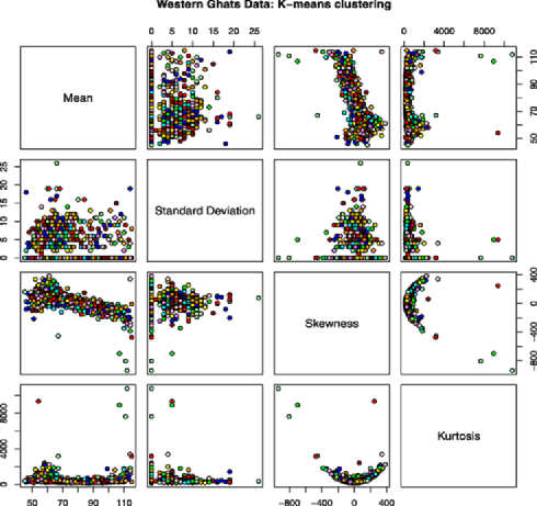
Figure 1: Pairwise scatterplots of the 4-variables used for clustering the Western Ghats data. Different colours denote different clusters corresponding to the $K$-means clustering shown in Figure 2.

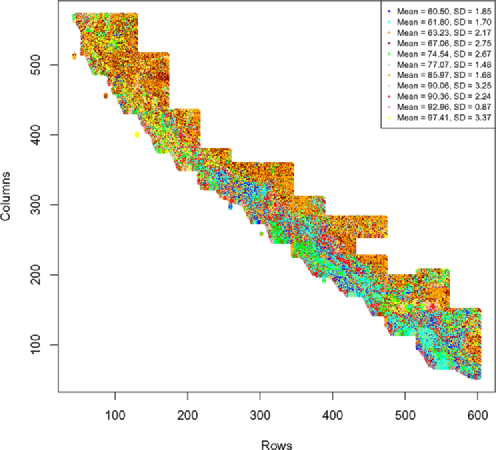
Figure 2: $K$-means clustering; different colours denote 11 different clusters. Cluster averages of mean (Mean) and standard deviation (SD) are shown in the legend.

The pairwise scatterplots of the four variables used for clustering the Western Ghats data is shown in Figure 1. Only for this plotting purpose, the data set is thinned to include 1 four-variate observation in every 50 such observations. The data points within the scatterplots are colored differently to show 11 different clusters, obtained using $K$-means clustering, a proxy for the method used by NG for their clustering. The $K$-means clustering, which has been analyzed in detail in subsequent subsections, is displayed in Figure 2. Each point in the latter figure corresponds to a 4-variate observation indexed by its position of the form $(i,j)$, where $i$ and $j$ represent the spatial coordinates, namely, row and column numbers, respectively, on a relevant spatial grid.

It is important to note that NG has ignored the spatial structure of the superpixels while analyzing the data. It was perhaps anticipated by NG that the clustering would not change nonnegligibly by incorporating the spatial locations because of the huge and quite informative data. The computational difficulties associated with spatial methods with data sets as huge as this may be another quite pragmatic reason. But whatever the reasons of NG, it is perhaps worth investigating statistically, whether or not omission of the spatial structure is inconsequential. To this end, we carried out a simple, informal test, reported in Section S-5. Since the test indicated insignificance of the spatial structure, we proceeded with the same data set used by NG.

5.2 Choice of prior

We chose $\bolds{\mu}_{0}$ and $\mathbf{S}$ to be the mean and the covariance matrix of the data, respectively, $s=4$, the minimum degrees of freedom required to make $\mathbf{G}_{0}$ well-defined, and $\psi=1$. These choices are natural, and in this Western Ghats example, with massive data, robustness of the priors is ensured. But appropriate choices of $M$ and the prior of $\alpha$ are important, and here we have been guided by the results obtained by NG. For instance, the final clustering obtained by NG, with their method that uses the $K$-means method and a subjective merging procedure, consists of 11 clusters. However, they initially started with 20 clusters, obtaining 11 clusters finally. In our model, we set $M=30$ to account for some extra uncertainty. In fact, a maximum of 30 components has also been used by Richardson and Green (1997) and SB. For the scale parameter $\alpha$ we considered the prior $\alpha\sim\operatorname{Gamma}(0.1,0.1)$, that is, a Gamma distribution with mean 1 and variance 10. This prior is reasonably close to noninformative, and, importantly, with these prior choices, 11 clusters get the maximum posterior mass, matching the number of clusters obtained by NG. A detailed study of sensitivity of the posterior inference with respect to other choices of the priors is reported in Section S-6.

5.3 Gibbs sampling for computing the posterior distribution of clustering

Apparently, for our purpose, the marginalized version of SB’s model described in Section 2 seems preferable since here we are only interested in the posterior distribution of clustering, and hence retaining the parameters $\bolds{\Theta}_{M}$ seems to serve no purpose. However, the expressions in Sections S-1 and S-2 show that calculation of the full conditional probabilities of $z_{i}$ in the marginalized version involves much more computational complexity compared to the nonmarginalized version. Since these computational complexities are multiplied $n$ times while updating the complete $\mathbf{Z}$ vector, with $n=51\mbox{,}834$, the marginalized version tends to be infeasible for massive data. Indeed, for the marginalized version, it took about 30 hours to complete just 10 iterations. We remark that implementation of EW’s model using the marginalized algorithm proposed in MacEachern (1994) took more than 39 hours to generate just 10 MCMC realizations. On the other hand, for the nonmarginalized version of SB’s model, generation of 30,000 MCMC samples, which includes a burn-in of 10,000, took just around 14 hours. In Section S-7 we provide a thorough account of the computational superiority of SB’s model compared to that of EW. Section S-8 provides a new method based on clusterings to assess convergence of our Gibbs sampler. Excellent convergence is indicated by this methodology.

5.4 Posterior distribution of the number of clusters

The posterior probabilities of the number of components being $\{6,\ldots,18\}$ are $\{0.00025,0.00395,\break 0.02955,\ 0.10600,\ 0.20815,\ 0.25135,\ 0.20715,\ 0.12190,\ 0.05205,\ 0.01555,\break 0.00345,0.00055,0.00010\}$, respectively, while the other values have zero posterior probabilities. Thus, 11 components have the maximum posterior probability, 0.25135. The components in this example all turned out to be nonempty, which is to be expected since the data set is so large. Even with other experiments with this data set, using SB’s model, this same fact was observed. Hence, we will use the terms “clusters” and “components” interchangeably from this point on. It is striking to note that NG also obtained 11 clusters with their analysis of the Western Ghats data.

5.5 Bayesian central clustering of the Western Ghats data

We obtained two central clusterings: the one obtained in the 759th iteration, corresponding to $\varepsilon=0.65$, which consists of 14 clusters, and another obtained in the 412th iteration, corresponding to $\varepsilon=0.70$, consisting of 10 clusters. It is worth noting that the empirical probabilities $\frac{1}{N}\#\{C^{(k)};1\leq k\leq N\dvtx\hat{d}(C^{(i)},\break C^{(k)})<\varepsilon\}$ for $i=1,\ldots,N$, turned out to be zero for $\varepsilon<0.65$. For $\varepsilon>0.70$ both clusterings corresponding to the 412th and the 759th iterations maximized the aforementioned empirical probabilities. Hence, the clustering corresponding to the 759th iteration is an estimate of the global mode of the posterior of clustering as it corresponds to the smaller $\varepsilon$. Figure 3 shows the clustering of the modal clustering, $C^{(412)}$. The other clustering, $C^{(759)}$, is displayed in Figure 4.

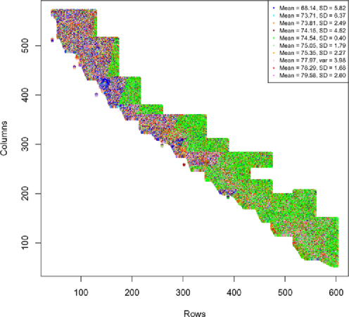
Figure 3: Modal central clustering $C^{(412)}$; different colours denote 10 different clusters. Cluster averages of mean (Mean) and standard deviation (SD) are shown in the legend.

Figure 4: Modal central clustering $C^{(759)}$; different colours denote 14 different clusters. Cluster averages of mean (Mean) and standard deviation (SD) are shown in the legend.

The two modal clusterings are close to each other, the distance being 0.649, even though the number of their clusters differ. Although one might suspect, because of the relative closeness of the two modes, that some clusters of the 10-cluster mode $C^{(412)}$ are simply split up to give rise to the 14-cluster mode $C^{(759)}$, this is not the case, as is also evident from the average means and average standard deviations reported in the legends of Figures 3 and 4. The average means and the average standard deviations of at least some clusterings would have been the same across the two figures had this been the case.

It is not surprising that the two central clusterings consist of 14 and 10 clusters, although 11 clusters have the maximum posterior probability. This is because the Bayesian central clustering has been obtained unconditionally, marginalizing over the number of components, without fixing the number of components at 11. This issue, concerning conditional and unconditional clusterings, will be discussed in detail in Section 5.8. Here we only note that the distance between two clusterings need not be small even if the number of clusters are the same (see the examples in Section 4.2); had this been the case, conditional and unconditional clusterings would be the same.

5.6 Bayesian 95% credible and HPD regions

Furthermore, with $\varepsilon^{*}=0.707$ and $\varepsilon^{*}=0.746$, we obtained approximately 95% credible regions corresponding to the central clusterings $C^{(412)}$ and $C^{(759)}$, respectively. In both cases the probability of the credible region turned out to be 0.951. Since the distance between $C^{(412)}$ and $C^{(759)}$ is 0.649, each falls within the 95% credible region of the other. We also constructed the 95% HPD region using the two central clusterings. Employing the adaptive algorithm provided in Section 3.4, we obtained $\varepsilon^{*}_{1}=0.688$ and $\varepsilon^{*}_{2}=0.710$ corresponding to $C^{(412)}$ and $C^{(759)}$, respectively. The probability of the HPD region is 0.952.

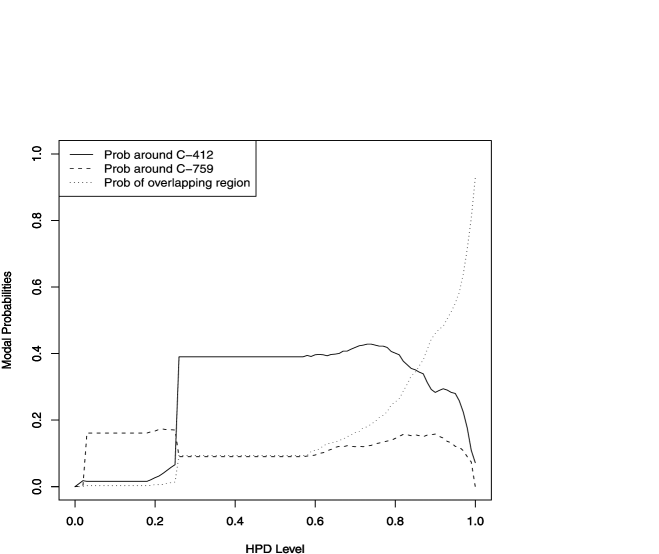
Figure 5: Plots of probabilities around each of the two modes $C^{(412)}$ and $C^{(759)}$ against the corresponding HPD levels. These probabilities exclude the probabilities of the intersection of the two modal regions given by $\operatorname{Pr}(\{C\dvtx\hat{d}(C^{(412)},C)<\varepsilon_{1}\}\cap\{C\dvtx\hat{d}(C^{(759)},C)<\varepsilon_{2}\})$, the values of which are plotted separately against the corresponding HPD levels for appropriate values of $\varepsilon_{1}$ and $\varepsilon_{2}$.

Figure 5 shows the probabilities around each of the two modal clusterings (excluding the probabilities of the overlapping regions) for different levels of HPD. The probabilities of the overlapping regions for different levels of HPD are also shown in the same figure. Initially, that is, when the HPD levels were less than 0.3, the probabilities around $C^{(759)}$ were greater than those around $C^{(412)}$, but from that point on the modal probabilities of $C^{(412)}$ were greater. This is not surprising, since $C^{(759)}$ is the global mode (see Section 5.5) implying that for smaller HPD levels most probability mass will be concentrated around its modal region. But since its modal region must be smaller compared to that of $C^{(412)}$, which is the local mode, for higher HPD levels the former can accommodate only a small portion of the entire HPD level. The remaining, larger portion of the HPD level must be associated with the modal region of the local mode. Also, as to be expected, the probabilities of the overlapping regions increased steadily with the HPD levels.

The distribution of the number of clusters of the clusterings fallingwithin the 95% HPD regions are as follows: the number of clusters getting nonzero probabilities are $\{7,\ldots,16\}$, and their respective probabilities are $\{0.004201681,\ 0.024159664,\ 0.101890756,\ 0.198529412,\ 0.255252101,\break 0.222689076,\ 0.122899160,\ 0.056722689,\ 0.009453782,\ 0.004201681\},$ showing that 11 clusters again receives the maximum probability.

5.7 Method of NG

NG essentially used a $K$-means clustering algorithm [see, e.g., Hartigan (1975)], fixing the number of clusters to be 20. Next, 14 clusters were obtained by merging some of the final 20 clusters. These were further reduced to 11 clusters, the merging operation justified on ecological grounds, rather than classical statistical theory of clustering. We interpret this “ecological justification of merging” as implicit use of subjective prior information. Since the numerical results or the exact methodological steps of NG are not available to us, we used the $K$-means algorithm with the number of clusters set equal to 11, as a proxy for the methodology of NG. Figure 2 displays the $K$-means clustering of the Western Ghats data set. We, however, found that the distance from the $K$-means clustering to $C^{(759)}$ and $C^{(412)}$ are 0.832 and 0.848, respectively, signifying that the $K$-means clustering does not fall within the 95% credible or HPD regions corresponding to our Bayesian methodologies. The reasons for this discrepancy between our Bayesian central clustering and the $K$-means clustering are discussed in detail in Section 5.8.

5.8 Bayesian conditional and unconditional central clusterings and comparison with $K$-means clustering

The issue of conditioning of our Bayesian central clustering on $k$ clusters is the key to understanding the discrepancy between central clustering and $K$-means clustering, which we now discuss.

Our Bayesian method obtains central clustering by taking account of uncertainties about the number of clusters, while the $K$-means algorithm keeps the number of clusters fixed, thus failing, while clustering the data, to take account of the uncertainty involved in clustering. To vindicate this, we obtained Bayesian central clustering conditional on 11 components. The clustering in the very first iteration, denoted by $C^{(1)}$, now turned out to be the central clustering, and it remained so for all $\varepsilon\geq 0.75$. For $\varepsilon<0.75$ for any $i\in\{1,\ldots,N\}$, the empirical probabilities $\frac{1}{N}\#\{C^{(k)};1\leq k\leq N:\hat{d}(C^{(i)},C^{(k)})<\varepsilon\}$ turned out to be zero, suggesting that $C^{(1)}$ is the global mode, conditional on 11 clusters. The conditional central clustering $C^{(1)}$ is shown in Figure 6. The conditional 95% credible region, which is also the conditional 95% HPD region because of unimodality, is given by $\{C:\hat{d}(C^{(1)},C)<0.827\}$, for those $C$ having 11 clusters. The empirical probability of this set is 0.95, indicating very good approximation to the true credible region. Importantly, the $K$-means clustering now falls within this 95% credible region, the distance between $C^{(1)}$ and $K$-means clustering being 0.729. We remark in this context that the distance between the central clustering conditional on $k$ clusters and the $K$-means clustering with 11 clusters is minimized when $k=11$. That the unconditional 95% Bayesian credible region does not include the $K$-means clustering but this conditional 95% Bayesian credible region does shows that $K$-means clustering fails to account for the uncertainty in the number of clusters, even if one fixes the number of clusters very accurately in the $K$-means algorithm.

Figure 6: Modal conditional central clustering $C^{(1)}$; different colours denote 11 different clusters. The first component of each of the distinct mean values $\{\mu^{*}_{1j};j=1,\ldots,11\}$, associated with the clusters, are shown in the legend.

Hence, although the results of NG are not available to us, we can conclude, based on our analyses, that the clustering they obtained is unlikely to fall within our unconditional 95% credible or HPD regions, even though broadly their clustering, plotted as Figure 1 in NG, looks similar to our Figure 4. Their results are rather comparable with our conditional clustering, shown in Figure 6. Detailed interpretation of the results and their comparisons are provided in Section 6.

6 Detailed interpretation of the results of the Western Ghats data analysis

Following NG, we order the landscape types of Western Ghats in ascending order of the means (the first component of the 4-variate data vectors) within each cluster. Since the clusterings obtained by us need not match that obtained by NG, our ordering of the landscape types need not agree with that of NG. But in spite of this, the similarities between the clustering obtained by NG and our $K$-means clustering seem to be substantial. Details of landscape types and their comparisons with respect to different clusterings are presented below.

6.1 Landscape type-1

6.1.1 Distribution in $K$-means clustering

Landscape type-1 of our $K$-means clustering (Figure 2) is distributed mainly in the south-east, and toward the middle part of Western Ghats. Comparatively small parts of landscape 1 are also distributed in the south-west region, and are almost absent in the northern region. Fair amount of heterogeneity in this landscape type is indicated by the average standard deviation associated with this cluster. This shows that this landscape comprises a mixture of several ecosystems. From the description provided by NG about this part of Western Ghats (the location of landscape 1 of $K$-means clustering seems to correspond to the locations of landscapes 1 and 2 of NG), we can infer that the natural vegetation of the south-east part of this landscape area is tropical dry deciduous forest, where rice, millets and oilseeds are grown. The middle part of the Ghats where this landscape is also found comprises tropical moist deciduous forest. Large parts of this landscape have been converted to open areas with palmyra trees planted in between. The small south-western parts of this landscape consist of moist deciduous vegetation.

6.1.2 Distribution in conditional clustering

Landscape 1 of conditional clustering (Figure 6) is distributed all over Western Ghats (corresponding to either of the similar landscape types 4, 5, 6 of NG), and the high standard deviation indicates the very substantial number of ecosystems it comprises. Natural vegetation is mostly dry deciduous in the north and moist deciduous in the south. The forests of the north have been replaced by tree savanna, shrub savanna and open land complexes. The south consists of open lands and palmyra trees. Rice, millets and oilseeds are planted in some parts of this landscape. The eastern parts are of the montane wet evergreen forest type.

6.1.3 Distribution in clustering $C^{(412)}$

In the case of $C^{(412)}$ (Figure 3), landscape type 1 is distributed over the north-west part of the Ghats, and is absent elsewhere. High average standard deviation suggests that this landscape is a mixture of many individual landscape elements. This part is characterized by dry deciduous vegetation. As opposed to the previous clusterings, in this case landscape 1 does not seem to be consistent with any of the landscapes of NG.

6.1.4 Distribution in clustering $C^{(759)}$

Consistent with the case of $C^{(412)}$, here also landscape 1 is distributed mainly over the north-western part of Western Ghats, and here also the average standard deviation is quite high. Once again, this landscape is not consistent with any landscape obtained by NG.

6.2 Landscape type-2

6.2.1 Distribution in $K$-means clustering

The distribution of landscape type 2 for $K$-means clustering is similar to that of landscape type 1. The average standard deviation is also comparable, and is only slightly less.

6.2.2 Distribution in conditional clustering

The distribution in this case is comparable to that of landscape 1 of conditional clustering, only the variability is much less, suggesting that fewer ecosystems have comprised this landscape.

6.2.3 Distribution in clustering $C^{(412)}$

In the case of $C^{(412)}$, landscape 2 is distributed mainly along the north-western part, stretching along the mid-western part of the Ghats, and also comprising some part of the south-eastern part. The large variability suggests abundance of individual landscape elements. The natural vegetation here is dry deciduous forests in the north and moist deciduous forests toward the south.

6.2.4 Distribution in clustering $C^{(759)}$

Landscape 2 for $C^{(759)}$ stretches mainly from the middle part of the Western Ghats extending till south, where it is more prominent. Here also the variability is significant, although smaller compared to that of $C^{(412)}$. The vegetation here is mainly tropical and moist deciduous forests.

6.3 Landscape type-3

6.3.1 Distribution in $K$-means clustering

Landscape type 3, as also in the case of landscape type 3 of NG, is present mainly along the eastern sides of Western Ghats. The natural vegetation is of the montane wet evergreen and moist deciduous forest type, and rice, millets and oilseeds are grown.

6.3.2 Distribution in conditional clustering

With respect to the conditional clustering, landscape type 3 is distributed along the entire length of the Western Ghats, not mainly toward the eastern part as in the case of $K$-means clustering.

6.3.3 Distribution in clustering $C^{(412)}$

With respect to $C^{(412)}$, this landscape is distributed mainly toward the eastern part of the Ghats, but also generally along the entire region.

6.3.4 Distribution in clustering $C^{(759)}$

As in the previous clusterings, landscape 3 is distributed mainly along the eastern side of the Ghats with respect to $C^{(759)}$. The variability in this case is a little less than in the case of other clusterings.

6.4 Landscape type-4

6.4.1 Distribution in $K$-means clustering

As in the case of corresponding landscape 3, landscape 4 for $K$-means is also distributed mainly toward the eastern region, and in the northern part it is distributed in both eastern and western parts, showing similarity with the distribution of landscape 4 of NG. The variability is large enough to suggest prevalence of a number of different ecosystems.

6.4.2 Distribution in conditional clustering

Landscape 4 of the conditional clustering has a distribution similar to that of the corresponding landscape 3. The variability is higher than in the case of landscape 3 of this clustering.

6.4.3 Distribution in clustering $C^{(412)}$

This landscape is present mainly along the north-western and the mid-eastern region of the Western Ghats, with variability higher than that of landscape 3 of $K$-means and the conditional clustering. The vegetation is mainly dry deciduous in the north-west and wet evergreen in the mid-east.

6.4.4 Distribution in clustering $C^{(759)}$

The distribution of landscape 4 of $C^{(759)}$ is very similar to that of landscape 4 of $C^{(412)}$, but the variability is higher.

6.5 Landscape type-5

6.5.1 Distribution in $K$-means clustering

As in the case of landscape 5 of NG, here also landscape 5 is distributed along the entire length of the Western Ghats, but more toward the western side, rather than the eastern side as found by NG in their landscape 5. A number of individual landscape elements are indicated by the mean standard deviation.

6.5.2 Distribution in conditional clustering

Landscape 5 associated with the conditional clustering is distributed along the entire Western Ghats, and has smaller variability than landscape 5 of the $K$-means clustering.

6.5.3 Distribution in clustering $C^{(412)}$

For $C^{(412)}$ landscape 5 is present mainly in the eastern parts and in the southern foothills. The mean standard deviation is even smaller than landscape 5 of the conditional clustering. The natural vegetation is wet evergreen and moist deciduous forests.

6.5.4 Distribution in clustering $C^{(759)}$

The distribution of landscape 5 of $C^{(759)}$ resembles that of landscape 5 of $C^{(412)}$, although the distribution of the former is less prominent in the eastern side and the southern foothills. The mean standard deviation is not that significant, although it is higher than in landscape 5 of $C^{(412)}$.

6.6 Landscape type-6

6.6.1 Distribution in $K$-means clustering

The distribution of landscape 6 of the $K$-means clustering is over the entire Western Ghats, similar to the distribution of landscape 6 of NG, but toward the south it is distributed more in the west, rather than in the east, as in NG. In the north, the distribution is more toward the east, rather than toward the west coast, as in NG. The mean standard deviation being 1.48 is not that significant.

6.6.2 Distribution in conditional clustering

Landscape 6 of the conditional clustering is distributed along the entire length of the Western Ghats, with higher mean standard deviation compared to landscape 6 of the $K$-means clustering.

6.6.3 Distribution in clustering $C^{(412)}$

Here the distribution is again over the entire Ghats, but with larger mean standard deviation compared to landscape 6 of the conditional clustering.

6.6.4 Distribution in clustering $C^{(759)}$

The distribution of landscape 6 of $C^{(759)}$ is mainly in the northern, north-western and mid-western region of the Western Ghats, with significantly high mean standard deviation, suggesting a large number of individual landscape elements. The natural vegetation is dry deciduous and evergreen.

6.7 Landscape type-7

6.7.1 Distribution in $K$-means clustering

Very closely resembling landscape 7 of NG, landscape type 7 of the $K$-means clustering is distributed both to the east and west of the entire Western Ghats. Here the natural vegetation is of the wet evergreen type, extending to moist deciduous in the southern part of the Western Ghats. It is this landscape within which, according to NG, most evergreen forests of the Western Ghats fall. The natural vegetation has been replaced to a large extent by woodland to savanna-woodland, tree savanna to grass savanna, thickets and scattered shrubs. As for the crops, millets, cotton and rice are grown in the north while millets and oilseeds are grown in the south. Arecanut, coconut, coffee, etc. are also grown in this landscape. The mean standard deviation being 1.68 does not indicate a large number of ecosystems.

6.7.2 Distribution in conditional clustering

Landscape 7 of the conditional clustering is again distributed all over Western Ghats. The mean standard deviation is somewhat large, suggesting quite a few individual landscape elements.

6.7.3 Distribution in clustering $C^{(412)}$

The distribution of landscape 7 of $C^{(412)}$ resembles that of landscape 7 of the conditional clustering. The mean standard deviations are also similar.

6.7.4 Distribution in clustering $C^{(759)}$

Landscape type 7 of $C^{(759)}$ resembles landscape type 7 of the conditional clustering and $C^{(412)}$, but it is distributed more prominently toward the north-east and the southern parts of the Ghats. The natural vegetation is mainly dry deciduous and evergreen, extending to moist deciduous in the south. The mean standard deviation being small does not indicate too many ecosystems.

6.8 Landscape type-8

6.8.1 Distribution in $K$-means clustering

Landscape 8 with respect to the $K$-means clustering is mainly present in the western part of the northern regions and both eastern and western parts of the middle and southern regions. This is unlike the distribution of landscape 8 of NG, which is present mostly in the western part and absent in the north. Rather, the distribution of landscape 8 of the $K$-means clustering resembles landscape 7 of the $K$-means clustering and that of NG. The mean standard deviation is, however, higher in this case.

6.8.2 Distribution in conditional clustering

The distribution of landscape 8 of the conditional clustering closely resembles the distributions of the previous landscapes of the same clustering. The mean standard deviation does not indicate too many ecosystems.

6.8.3 Distribution in clustering $C^{(412)}$

Landscape type 8 of $C^{(412)}$ is present most in the northern and north-western regions of the Western Ghats. The vegetation is mostly dry deciduous. The variability is significant, indicating many ecosystems.

6.8.4 Distribution in clustering $C^{(759)}$

Landscape type 8 of $C^{(759)}$ is distributed mainly along the northern, north-western and mid-western regions of the Ghats. The vegetation is mainly dry deciduous, extending to evergreen. The variability is high, suggesting many ecosystems.

6.9 Landscape type-9

6.9.1 Distribution in $K$-means clustering

Agreeing very closely with NG, landscape type 9 of $K$-means clustering is nearly absent in the northern stretches and is present in the central and southern parts in patches toward the west. Here the natural vegetation is evergreen and semi-evergreen. Disturbed semi-evergreen forests along with moist deciduous forests, woodlands and savanna-woodlands are also present. Crops like rice, tapioca, coconut, millets and oilseeds are grown. Relatively high mean standard deviation suggests a mixture of several ecosystems.

6.9.2 Distribution in conditional clustering

The distribution of landscape 9 of the conditional clustering is all over the Ghats, but in the mid-western regions the distribution is more prominent. The vegetation in this region is evergreen. The variability suggests several individual landscape elements.

6.9.3 Distribution in clustering $C^{(412)}$

Landscape 9 of $C^{(412)}$ is distributed all over the Ghats but is present more prominently toward the eastern parts. Not many individual landscape types are indicated by the mean standard deviation.

6.9.4 Distribution in clustering $C^{(759)}$

Landscape 9 of $C^{(759)}$ is distributed all over the Ghats but is present more prominently toward the western parts. Quite a few individual landscape types are indicated by the mean standard deviation.

6.10 Landscape type-10

6.10.1 Distribution in $K$-means clustering

Landscape type 10 is present in a few patches toward the northern and in the central parts of the Ghats. The vegetation is evergreen. The low mean standard deviation does not suggest much heterogeneity.

6.10.2 Distribution in conditional clustering

In the conditional clustering, landscape type 10 is found mainly in the north-western, mid-western and in the southern parts of Western Ghats. The vegetation ranges between dry deciduous, evergreen and moist deciduous. Here also relative homogeneity is indicated by the low mean standard deviation.

6.10.3 Distribution in clustering $C^{(412)}$

In $C^{(412)}$ landscape type 10 is present mainly in the western part along the entire length of the Ghats. The natural vegetation is deciduous as well as evergreen. Among crops, rice, tapioca and coconut are planted. The variability suggests nonnegligible heterogeneity.

6.10.4 Distribution in clustering $C^{(759)}$

Landscape type 10 with respect to $C^{(759)}$ is mostly present in the mid-eastern regions and the southern part of the Western Ghats. The natural vegetation is wet evergreen and moist deciduous. Not much heterogeneity is indicated by the mean standard deviation.

6.11 Landscape type-11

6.11.1 Distribution in $K$-means clustering

In contrast with landscape type 11 of NG, which is present in a single patch, here it is present in the northern stretches, and in the eastern stretches of the central and the southern parts of Western Ghats. The vegetation varies from dry deciduous to moist deciduous forests, with wet evergreen forests in the mid-eastern parts. A fair amount of heterogeneity is indicated by the mean standard deviation.

6.11.2 Distribution in conditional clustering

Landscape type 11 associated with the conditional clustering is present mainly in the mid-eastern and the southern parts of the Ghats. The vegetation here is mostly wet evergreen and moist deciduous. A fair amount of homogeneity is indicated by the mean standard deviation.

6.11.3 Distribution in clustering $C^{(759)}$

Landscape 11 of $C^{(759)}$ is present all over Western Ghats but is more prominent toward the mid-eastern and the southern parts, as in the case of landscape 11 of the conditional clustering. A fair amount of individual landscape types are indicated by the variability.

6.12 Landscape type-12 of $C^{(759)}$

Landscape type 12 of $C^{(759)}$, in spite of its presence all over the Ghats, is more prominent in the mid-western and the south-western stretches. The natural vegetation is mainly evergreen and moist deciduous. Again, a fair amount of individual landscape types are suggested by the variability.

6.13 Landscape type-13 of $C^{(759)}$

This landscape is present mainly in the central and the southern parts of the Ghats, with mostly evergreen and moist deciduous vegetation. A very low mean standard deviation indicates homogeneity.

6.14 Landscape type-14 of $C^{(759)}$

This landscape is present all over Western Ghats, but mainly along the western stretches and in the southern foothills. The vegetation is dry deciduous in the north, evergreen in the center and moist deciduous in the south. The mean standard deviation indicates some amount of heterogeneity.

7 Conclusion

We have highlighted the importance of acknowledging clustering uncertainty, and have introduced methodologies for summarizing posterior distributions of clusterings. We have demonstrated how central clusterings can be obtained from posterior samples drawn using MCMC methodologies. In the heart of our proposed methods for summarizing posterior distributions of clusterings is a clustering metric introduced to compare any two clusterings. Although computation of the exact distance between two clusterings can be expensive, we have introduced a computationally cheap, and perhaps, more importantly, accurate, approximation to the exact metric. We remark that although we have confined our attention to the modes of the posterior distribution of clusterings in this paper, it is also possible to obtain the median of the posterior distribution of clusterings. For instance, the median $C^{(\mathrm{med})}$ may be defined as $C^{(\mathrm{med})}=\arg\min_{C}\sum_{i=1}^{N}\hat{d}(C^{(i)},C)$. Also, considering any “reference clustering” $C^{(0)}$, acting as the origin, a partial ordering “$\preceq$” with respect to the origin can be defined on the set of the clusterings obtained from MCMC sampling as $C^{(i)}\preceq C^{(j)}$ if and only if $\hat{d}(C^{(0)},C^{(i)})\leq\hat{d}(C^{(0)},C^{(j)})$, for any $i,j$. Using this partial ordering, any quantile with respect to the origin can be calculated.

Analysis of the Western Ghats data based on our proposed methodologies revealed broad similarities with the results obtained by NG, which includes the number of clusters obtained by them is the one which gets the highest posterior probability corresponding to our Bayesian model. However, we have also pointed out that the clustering obtained by NG is unlikely to fall within our unconditional 95% credible or HPD regions, although it is likely to fall within our conditional 95% credible or HPD regions, conditioned on the number of clusters, fixed in their deterministic algorithm. Such a drawback, as we have shown, is due to the failure of the deterministic algorithm to take account of the uncertainty involved with the number of clusters. The detailed results of our application to the biodiversity hotspot Western Ghats reveal dissimilarities of the landscape types obtained by our clustering methodology with that obtained by a proxy to NG’s clustering algorithm. As to be expected, some similarity is exhibited between the landscape types obtained by these methods, when we conditioned on the same number of clusters fixed by NG. These new and interesting facts indicate that ecologists may need to update their methodologies for studying biodiversity. The methodologies we proposed in this paper are not expected to be immediately accessible to ecologists because of the technical gap between ecological and statistical communities, but collaborative efforts may yield fruit in the future, benefitting both communities.

References

- Antoniak (1974) {barticle}[author] \bauthor\bsnmAntoniak, \bfnmC. E.\binitsC. E. (\byear1974). \btitleMixtures of Dirichlet processes with applications to nonparametric problems. \bjournalAnn. Statist. \bvolume2 \bpages1152–1174. \MR0365969 \endbibitem
- Berger (1985) {bbook}[author] \bauthor\bsnmBerger, \bfnmJ. O.\binitsJ. O. (\byear1985). \btitleStatistical Decision Theory and Bayesian Analysis, \bedition2nd ed. \bpublisherSpringer, \baddressNew York. \MR0804611 \endbibitem
- Bhattacharya (2008) {barticle}[author] \bauthor\bsnmBhattacharya, \bfnmS.\binitsS. (\byear2008). \btitleGibbs sampling based Bayesian analysis of mixtures with unknown number of components. \bjournalSankhyā Ser. B \bvolume70 \bpages133–155. \MR2507480 \endbibitem
- Dahl (2009) {barticle}[author] \bauthor\bsnmDahl, \bfnmD. B.\binitsD. B. (\byear2009). \btitleModal clustering in a class of product partition models. \bjournalBayesian Anal. \bvolume4 \bpages243–264. \endbibitem
- Escobar and West (1995) {barticle}[author] \bauthor\bsnmEscobar, \bfnmM. D.\binitsM. D. and \bauthor\bsnmWest, \bfnmM.\binitsM. (\byear1995). \btitleBayesian density estimation and inference using mixtures. \bjournalJ. Amer. Statist. Assoc. \bvolume90 \bpages577–588. \MR1340510 \endbibitem
- Ferguson (1973) {barticle}[author] \bauthor\bsnmFerguson, \bfnmT. S.\binitsT. S. (\byear1973). \btitleA Bayesian analysis of some nonparametric problems. \bjournalAnn. Statist. \bvolume1 \bpages209–230. \MR0350949 \endbibitem
- Fraley and Raftery (1999) {barticle}[author] \bauthor\bsnmFraley, \bfnmC.\binitsC. and \bauthor\bsnmRaftery, \bfnmA. E.\binitsA. E. (\byear1999). \btitleMCLUST: Software for model-based cluster analysis. \bjournalJ. Classification \bvolume16 \bpages297–306. \endbibitem
- Fraley and Raftery (2002) {barticle}[author] \bauthor\bsnmFraley, \bfnmC.\binitsC. and \bauthor\bsnmRaftery, \bfnmA. E.\binitsA. E. (\byear2002). \btitleModel-based clustering, discriminant analysis, and density estimation. \bjournalJ. Amer. Statist. Assoc. \bvolume97 \bpages611–631. \MR1951635 \endbibitem