Mask Iterative Hard Thresholding Algorithms for Sparse Image Reconstruction of Objects with Known Contour^†

Abstract

We develop mask iterative hard thresholding algorithms (mask IHT and mask DORE) for sparse image reconstruction of objects with known contour. The measurements follow a noisy underdetermined linear model common in the compressive sampling literature. Assuming that the contour of the object that we wish to reconstruct is known and that the signal outside the contour is zero, we formulate a constrained residual squared error minimization problem that incorporates both the geometric information (i.e. the knowledge of the object’s contour) and the signal sparsity constraint. We first introduce a mask IHT method that aims at solving this minimization problem and guarantees monotonically non-increasing residual squared error for a given signal sparsity level. We then propose a double overrelaxation scheme for accelerating the convergence of the mask IHT algorithm. We also apply convex mask reconstruction approaches that employ a convex relaxation of the signal sparsity constraint. In X-ray computed tomography (CT), we propose an automatic scheme for extracting the convex hull of the inspected object from the measured sinograms; the obtained convex hull is used to capture the object contour information. We compare the proposed mask reconstruction schemes with the existing large-scale sparse signal reconstruction methods via numerical simulations and demonstrate that, by exploiting both the geometric contour information of the underlying image and sparsity of its wavelet coefficients, we can reconstruct this image using a significantly smaller number of measurements than the existing methods.

I Introduction

Compressive sampling exploits the fact that most natural signals are well described by only a few significant (in magnitude) coefficients in some [e.g. discrete wavelet transform (DWT)] domain, where the number of significant coefficients is much smaller than the signal size. Therefore, for an $p\times 1$ vector $x$ representing the signal and an appropriate $p\times p$ sparsifying transform matrix ${\mathit{\Psi}}$, we have $\mbox{\boldmath$x$}={\mathit{\Psi}}\,\mbox{\boldmath$s$}$, where $\mbox{\boldmath$s$}=[s_{1},s_{2},\ldots,s_{p}]^{T}$ is an $p\times 1$ signal transform-coefficient vector with most elements having small magnitudes. The idea behind compressive sampling or compressed sensing is to sense the significant components of $s$ using a small number of linear measurements:

$$\mbox{\boldmath$y$}={\mathit{\Phi}}\,\mbox{\boldmath$x$}$$ (1)

where $y$ is an $N\times 1$ measurement vector and ${\mathit{\Phi}}$ is a known $N\times p$ sampling matrix with $N\leq p$; here, we focus on the scenario where the measurements, signal coefficients, and sampling and sparsifying transform matrices are real-valued. Practical recovery algorithms, including convex relaxation, greedy pursuit, and probabilistic methods, have been proposed to find the sparse solution to the underdetermined system (1), see [1] for a survey.

Compressive sampling takes the advantage of the prior knowledge that most natural signals are sparse in some transform domain. In addition to the signal sparsity, we use geometric constraints to enhance the signal reconstruction performance. In particular, we assume that the contour of the object under inspection is known and that the signal outside the contour is zero. A convex relaxation method was outlined in [2] for image reconstruction with both sparsity and object contour information. (Note that [2] does not provide sufficient information to replicate its results and, furthermore, the method’s development in [2, eqs. (4)–(6)] clearly contains typos or errors.) Here, we propose (i) iterative hard thresholding and convex relaxation algorithms that incorporate the object’s contour information into the signal reconstruction process and (ii) an automatic scheme for extracting the convex hull of the inspected object (which captures the object contour information) from the measured X-ray computed tomography (CT) sinograms.

We introduce our measurement model in Section II and the proposed iterative hard thresholding methods in Section III. Our mask convex relaxation algorithms are described in Section IV. The experimental results are given in Section VI.

We introduce the notation: $\|\cdot\|_{p}$ and “^T” denote the $\ell_{p}$ norm and transpose, respectively, and the sparse thresholding operator ${\cal T}_{r}(\mbox{\boldmath$s$})$ keeps the $r$ largest-magnitude elements of a vector $s$ intact and sets the rest to zero, e.g. ${\cal T}_{2}([0,1,-5,0,3,0]^{T})=[0,0,-5,0,3,0]^{T}$. The largest singular value of a matrix $H$ is denoted by $\rho_{{\scriptstyle{\it H}}}$ and is also known as the spectral norm of $H$. Finally, $I_{n}$ and ${\bf 0}_{n\times 1}$ denote the identity matrix of size $n$ and the $n\times 1$ vector of zeros, respectively.

II Measurement Model

We incorporate the geometric constraints via the following signal model: the elements of the $p\times 1$ signal vector $\mbox{\boldmath$x$}=[x_{1},x_{2},\ldots,x_{p}]^{T}$ are

$$x_{i}=\left\{\begin{array}[]{cc}[{\mathit{\Psi}}\,\mbox{\boldmath$s$}]_{i},&i\in\mathrm{M}\\ 0,&i\notin\mathrm{M}\end{array}\right.$$ (2)

for $i=1,2,\ldots,p$, where $[{\mathit{\Psi}}\,\mbox{\boldmath$s$}]_{i}$ denotes the $i$th element of the vector ${\mathit{\Psi}}\,\mbox{\boldmath$s$}$, the mask $\mathrm{M}$ is the set of $p_{{\scriptstyle{\rm M}}}\leq p$ indices corresponding to the signal elements inside the contour of the inspected object, $s$ is the $p\times 1$ sparse signal transform-coefficient vector, and ${\mathit{\Psi}}$ is the known orthogonal sparsifying transform matrix satisfying

$${\mathit{\Psi}}\,{\mathit{\Psi}}^{T}={\mathit{\Psi}}^{T}\,{\mathit{\Psi}}=I_{p}.$$ (3)

Therefore, the $p_{{\scriptstyle{\rm M}}}\times 1$ vector of signal elements inside the mask $\mathrm{M}$ ($x_{i},\,i\in\mathrm{M}$) is $\mbox{\boldmath$x$}_{{\scriptstyle{\rm M}}}={\mathit{\Psi}}_{{\scriptstyle{\rm M}},:}\,\mbox{\boldmath$s$}$, where the $p_{{\scriptstyle{\rm M}}}\times p$ matrix ${\mathit{\Psi}}_{{\scriptstyle{\rm M}},:}$ contains the $p_{{\scriptstyle{\rm M}}}$ rows of ${\mathit{\Psi}}$ that correspond to the signal indices within the mask $\mathrm{M}$. If the resulting ${\mathit{\Psi}}_{{\scriptstyle{\rm M}},:}$ has zero columns, the elements of $s$ corresponding to these columns are not identifiable and are known to be zero because they describe part of the image outside the mask $\mathrm{M}$. Define the set of indices $\mathrm{I}$ of nonzero columns of ${\mathit{\Psi}}_{{\scriptstyle{\rm M}},:}$ containing $p_{{\scriptstyle{\rm I}}}\leq p$ elements and the corresponding $p_{{\scriptstyle{\rm I}}}\times 1$ vector $\mbox{\boldmath$s$}_{{\scriptstyle{\rm I}}}$ of identifiable signal transform coefficients under our signal model. Then,

$$\mbox{\boldmath$x$}_{{\scriptstyle{\rm M}}}={\mathit{\Psi}}_{{\scriptstyle{\rm M}},{\scriptstyle{\rm I}}}\,\mbox{\boldmath$s$}_{{\scriptstyle{\rm I}}}$$ (4)

where the $p_{{\scriptstyle{\rm M}}}\times p_{{\scriptstyle{\rm I}}}$ matrix ${\mathit{\Psi}}_{{\scriptstyle{\rm M}},{\scriptstyle{\rm I}}}$ is the restriction of ${\mathit{\Psi}}_{{\scriptstyle{\rm M}},:}$ to the index set $\mathrm{I}$ and consists of the $p_{{\scriptstyle{\rm I}}}$ nonzero columns of ${\mathit{\Psi}}_{{\scriptstyle{\rm M}},:}$. Now, the noiseless measurement equation (1) becomes [see also (2) and (4)]

$$\mbox{\boldmath$y$}={\mathit{\Phi}}\,\mbox{\boldmath$x$}={\mathit{\Phi}}_{:,{\scriptstyle{\rm M}}}\,{\mathit{\Psi}}_{{\scriptstyle{\rm M}},{\scriptstyle{\rm I}}}\,\mbox{\boldmath$s$}_{{\scriptstyle{\rm I}}}$$ (5)

where the $N\times p_{{\scriptstyle{\rm M}}}$ matrix ${\mathit{\Phi}}_{:,{\scriptstyle{\rm M}}}$ is the restriction of the full sampling matrix ${\mathit{\Phi}}$ to the mask index set $\mathrm{M}$ and consists of the $p_{{\scriptstyle{\rm M}}}$ columns of the full sampling matrix ${\mathit{\Phi}}$ that correspond to the signal indices within $\mathrm{M}$. We now employ (5) and formulate the following constrained residual squared error minimization problem that incorporates both the geometric information (i.e. the knowledge of the inspected object’s contour) and the signal sparsity constraint:

$$({\rm P}_{0}):\quad\quad\min_{\mbox{\boldmath$s$}_{{\scriptstyle{\rm I}}}}\|\mbox{\boldmath$y$}-H\,\mbox{\boldmath$s$}_{{\scriptstyle{\rm I}}}\|_{2}^{2}\quad\mbox{subject to}\,\,\|\mbox{\boldmath$s$}_{{\scriptstyle{\rm I}}}\|_{0}\leq r$$ (6)

where $\|\mbox{\boldmath$s$}_{{\scriptstyle{\rm I}}}\|_{0}$ counts the number of nonzero elements in the vector $\mbox{\boldmath$s$}_{{\scriptstyle{\rm I}}}$ and $H={\mathit{\Phi}}_{:,{\scriptstyle{\rm M}}}\,{\mathit{\Psi}}_{{\scriptstyle{\rm M}},{\scriptstyle{\rm I}}}$. We refer to $r$ as the signal sparsity level and assume that it is known. Finding the exact solution to (6) involves a combinatorial search and is therefore intractable in practice. In the following, we present greedy iterative schemes that aim at solving (6).

III Mask IHT and Mask DORE

We first introduce a mask iterative hard thresholding (mask IHT) method and then propose its double overrelaxation acceleration termed mask DORE.

Assume that the signal transform coefficient estimate $\mbox{\boldmath$s$}_{{\scriptstyle{\rm I}}}^{(q)}$ is available, where $q$ denotes the iteration index. Iteration $(q+1)$ of our mask IHT scheme proceeds as follows:

$$\mbox{\boldmath$s$}_{{\scriptstyle{\rm I}}}^{(q+1)}={\cal T}_{r}\big{(}\mbox{\boldmath$s$}_{{\scriptstyle{\rm I}}}^{(q)}+\mu^{(q)}\,H^{T}\,(\mbox{\boldmath$y$}-H\,\mbox{\boldmath$s$}_{{\scriptstyle{\rm I}}}^{(q)})\big{)}$$ (7)

where $\mu^{(q)}>0$ is a step size chosen to ensure monotonically decreasing residual squared error, see also Section III-A. Iterate until $\mbox{\boldmath$s$}_{{\scriptstyle{\rm I}}}^{(q+1)}$ and $\mbox{\boldmath$s$}_{{\scriptstyle{\rm I}}}^{(q)}$ do not differ significantly. Upon convergence of this iteration yielding $\mbox{\boldmath$s$}_{{\scriptstyle{\rm I}}}^{(+\infty)}$, construct an estimate of the signal vector $\mbox{\boldmath$x$}_{{\scriptstyle{\rm M}}}$ inside the mask $\mathrm{M}$ using ${\mathit{\Psi}}_{{\scriptstyle{\rm M}},{\scriptstyle{\rm I}}}\,\mbox{\boldmath$s$}_{{\scriptstyle{\rm I}}}^{(+\infty)}$. In [3], we consider (7) with constant $\mu^{(q)}$ (not a function of $q$) set to $\mu^{(q)}=1/\rho_{{\scriptstyle{\it\Phi}}}^{2}$. For the full mask $\mathrm{M}=\{1,2,\ldots,p\}$ and constant $\mu^{(q)}$, (7) reduces to the standard iterative hard thresholding (IHT) algorithm in [4].

We now propose our mask DORE iteration that applies two consecutive overrelaxation steps after one mask IHT step to accelerate the convergence of the mask IHT algorithm. These two overrelaxations use the identifiable signal coefficient estimates $\mbox{\boldmath$s$}_{{\scriptstyle{\rm I}}}^{(q)}$ and $\mbox{\boldmath$s$}_{{\scriptstyle{\rm I}}}^{(q-1)}$ from the two most recently completed mask DORE iterations. Iteration $(q+1)$ of our mask DORE scheme proceeds as follows:

1. Mask IHT step.

$$\mbox{\boldmath$\widehat{s}$}_{{\scriptstyle{\rm I}}}=\mbox{\boldmath$\widehat{s}$}_{{\scriptstyle{\rm I}}}(\mbox{\boldmath$s$}_{{\scriptstyle{\rm I}}}^{(q)},\mu^{(q)})={\cal T}_{r}\big{(}\mbox{\boldmath$s$}_{{\scriptstyle{\rm I}}}^{(q)}+\mu^{(q)}\,H^{T}\,(\mbox{\boldmath$y$}-H\,\mbox{\boldmath$s$}_{{\scriptstyle{\rm I}}}^{(q)})\big{)}$$ (8)

where $\mu^{(q)}>0$ is a step size chosen to ensure monotonically decreasing residual squared error, see also Section III-A.

2. First overrelaxation. Minimize the residual squared error $\|\mbox{\boldmath$y$}-H\,\mbox{\boldmath$s$}_{{\scriptstyle{\rm I}}}\|_{2}^{2}$ with respect to $\mbox{\boldmath$s$}_{{\scriptstyle{\rm I}}}$ lying on the straight line connecting $\mbox{\boldmath$\widehat{s}$}_{{\scriptstyle{\rm I}}}$ and $\mbox{\boldmath$s$}_{{\scriptstyle{\rm I}}}^{(q)}$:

$$\mbox{\boldmath$\bar{z}$}_{{\scriptstyle{\rm I}}}=\mbox{\boldmath$\widehat{s}$}_{{\scriptstyle{\rm I}}}+\alpha_{1}\,(\mbox{\boldmath$\widehat{s}$}_{{\scriptstyle{\rm I}}}-\mbox{\boldmath$s$}_{{\scriptstyle{\rm I}}}^{(q)})$$ (9a)

which has a closed-form solution:

$$\alpha_{1}=\frac{(H\,\mbox{\boldmath$\widehat{s}$}_{{\scriptstyle{\rm I}}}-H\,\mbox{\boldmath$s$}_{{\scriptstyle{\rm I}}}^{(q)})^{T}\,(\mbox{\boldmath$y$}-H\,\mbox{\boldmath$\widehat{s}$}_{{\scriptstyle{\rm I}}})}{\|H\,\mbox{\boldmath$\widehat{s}$}_{{\scriptstyle{\rm I}}}-H\,\mbox{\boldmath$s$}_{{\scriptstyle{\rm I}}}^{(q)}\|_{2}^{2}}.$$ (9b)

3. Second overrelaxation. Minimize the residual squared error $\|\mbox{\boldmath$y$}-H\,\mbox{\boldmath$s$}_{{\scriptstyle{\rm I}}}\|_{2}^{2}$ with respect to $\mbox{\boldmath$s$}_{{\scriptstyle{\rm I}}}$ lying on the straight line connecting $\mbox{\boldmath$\bar{z}$}_{{\scriptstyle{\rm I}}}$ and $\mbox{\boldmath$s$}_{{\scriptstyle{\rm I}}}^{(q-1)}$:

$$\mbox{\boldmath$\widetilde{z}$}_{{\scriptstyle{\rm I}}}=\mbox{\boldmath$\bar{z}$}_{{\scriptstyle{\rm I}}}+\alpha_{2}\,(\mbox{\boldmath$\bar{z}$}_{{\scriptstyle{\rm I}}}-\mbox{\boldmath$s$}_{{\scriptstyle{\rm I}}}^{(q-1)})$$ (10a)

which has a closed-form solution:

$$\alpha_{2}=\frac{(H\,\mbox{\boldmath$\bar{z}$}_{{\scriptstyle{\rm I}}}-H\,\mbox{\boldmath$s$}_{{\scriptstyle{\rm I}}}^{(q-1)})^{T}\,(\mbox{\boldmath$y$}-H\,\mbox{\boldmath$\bar{z}$}_{{\scriptstyle{\rm I}}})}{\|H\,\mbox{\boldmath$\bar{z}$}_{{\scriptstyle{\rm I}}}-H\,\mbox{\boldmath$s$}_{{\scriptstyle{\rm I}}}^{(q-1)}\|_{2}^{2}}.$$ (10b)

4. Thresholding. Threshold $\mbox{\boldmath$\widetilde{z}$}_{{\scriptstyle{\rm I}}}$ to the sparsity level $r$: $\mbox{\boldmath$\widetilde{s}$}_{{\scriptstyle{\rm I}}}={\cal T}_{r}(\mbox{\boldmath$\widetilde{z}$}_{{\scriptstyle{\rm I}}})$.

5. Decision. If $\|\mbox{\boldmath$y$}-H\,\mbox{\boldmath$\widetilde{s}$}_{{\scriptstyle{\rm I}}}\|_{2}^{2}<\|\mbox{\boldmath$y$}-H\,\mbox{\boldmath$\widehat{s}$}_{{\scriptstyle{\rm I}}}\|_{2}^{2}$, assign $\mbox{\boldmath$s$}_{{\scriptstyle{\rm I}}}^{(q+1)}=\mbox{\boldmath$\widetilde{s}$}_{{\scriptstyle{\rm I}}}$; otherwise, assign $\mbox{\boldmath$s$}_{{\scriptstyle{\rm I}}}^{(q+1)}=\mbox{\boldmath$\widehat{s}$}_{{\scriptstyle{\rm I}}}$ and complete Iteration $q+1$.

Iterate until $\mbox{\boldmath$s$}_{{\scriptstyle{\rm I}}}^{(q+1)}$ and $\mbox{\boldmath$s$}_{{\scriptstyle{\rm I}}}^{(q)}$ do not differ significantly. As before, upon convergence of this iteration yielding $\mbox{\boldmath$s$}_{{\scriptstyle{\rm I}}}^{(+\infty)}$, construct an estimate of the signal vector $\mbox{\boldmath$x$}_{{\scriptstyle{\rm M}}}$ inside the mask $\mathrm{M}$ using ${\mathit{\Psi}}_{{\scriptstyle{\rm M}},{\scriptstyle{\rm I}}}\,\mbox{\boldmath$s$}_{{\scriptstyle{\rm I}}}^{(+\infty)}$.

III-A Step size selection

In Iteration 1 of our mask DORE and mask IHT schemes, we seek the largest step size $\mu^{(0)}$ that satisfies

$$\|\mbox{\boldmath$y$}-H\,\widehat{\mbox{\boldmath$s$}}_{{\scriptstyle{\rm I}}}\|_{2}^{2}\leq\|\mbox{\boldmath$y$}-H\,\mbox{\boldmath$s$}_{{\scriptstyle{\rm I}}}^{(0)}\|_{2}^{2}$$ (11)

where $\widehat{\mbox{\boldmath$s$}}_{{\scriptstyle{\rm I}}}=\mbox{\boldmath$\widehat{s}$}_{{\scriptstyle{\rm I}}}(\mbox{\boldmath$s$}_{{\scriptstyle{\rm I}}}^{(0)},\mu^{(0)})$ is computed using (8) with $q=0$. We achieve this goal approximately as follows: Start with an initial guess for $\mu^{(0)}>0$, compute the corresponding $\widehat{\mbox{\boldmath$s$}}_{{\scriptstyle{\rm I}}}=\mbox{\boldmath$\widehat{s}$}_{{\scriptstyle{\rm I}}}(\mbox{\boldmath$s$}_{{\scriptstyle{\rm I}}}^{(0)},\mu^{(0)})$, and

• if (11) holds for the initial step size guess, double (repeatedly, if needed) $\mu^{(0)}$ until the condition (11) for the corresponding $\widehat{\mbox{\boldmath$s$}}_{{\scriptstyle{\rm I}}}=\mbox{\boldmath$\widehat{s}$}_{{\scriptstyle{\rm I}}}(\mbox{\boldmath$s$}_{{\scriptstyle{\rm I}}}^{(0)},\mu^{(0)})$ fails;

• shrink (repeatedly, if needed) $\mu^{(0)}$ by multiplying it with $0.9$ until (11) for the corresponding $\widehat{\mbox{\boldmath$s$}}_{{\scriptstyle{\rm I}}}=\mbox{\boldmath$\widehat{s}$}_{{\scriptstyle{\rm I}}}(\mbox{\boldmath$s$}_{{\scriptstyle{\rm I}}}^{(0)},\mu^{(0)})$ holds;

• complete Iteration 1 by moving on to Steps 2–5 in mask DORE or setting $\mbox{\boldmath$s$}_{{\scriptstyle{\rm I}}}^{(q+1)}=\widehat{\mbox{\boldmath$s$}}_{{\scriptstyle{\rm I}}}$ in mask IHT.

In each subsequent Iteration $q+1$ ($q>0$), start with $\mu^{(q)}=\mu^{(q-1)}$, compute the corresponding $\widehat{\mbox{\boldmath$s$}}_{{\scriptstyle{\rm I}}}=\mbox{\boldmath$\widehat{s}$}_{{\scriptstyle{\rm I}}}(\mbox{\boldmath$s$}_{{\scriptstyle{\rm I}}}^{(q)},\mu^{(q)})$ in (8), and

• if

  $$\|\mbox{\boldmath$y$}-H\,\widehat{\mbox{\boldmath$s$}}_{{\scriptstyle{\rm I}}}\|_{2}^{2}\leq\|\mbox{\boldmath$y$}-H\,\mbox{\boldmath$s$}_{{\scriptstyle{\rm I}}}^{(q)}\|_{2}^{2}$$ (12)

  does not hold for the initial step size $\mu^{(q)}=\mu^{(q-1)}$, shrink $\mu^{(q)}$ by multiplying it (repeatedly, if needed) with $0.9$ until (12) for the corresponding $\widehat{\mbox{\boldmath$s$}}_{{\scriptstyle{\rm I}}}=\mbox{\boldmath$\widehat{s}$}_{{\scriptstyle{\rm I}}}(\mbox{\boldmath$s$}_{{\scriptstyle{\rm I}}}^{(q)},\mu^{(q)})$ holds;

• complete Iteration $q+1$ by moving on to Steps 2–5 in mask DORE or setting $\mbox{\boldmath$s$}_{{\scriptstyle{\rm I}}}^{(q+1)}=\widehat{\mbox{\boldmath$s$}}_{{\scriptstyle{\rm I}}}$ in mask IHT.

Therefore, our step size $\mu^{(q)}$ is a decreasing piecewise constant function of the iteration index $q$. The step size $\mu^{(+\infty)}$ obtained upon convergence (i.e. as $q\nearrow+\infty$) is larger than or equal to $0.9/\rho_{{\scriptstyle{\it H}}}^{2}$, which follows easily from Theorem 1 below.

Theorem 1

Assuming that

$$0<\mu^{(q)}\leq 1/\rho_{{\scriptstyle{\it H}}}^{2}$$ (13)

and that the signal coefficient estimate in the $q$-th iteration $\mbox{\boldmath$s$}_{{\scriptstyle{\rm I}}}^{(q)}$ belongs to the parameter space

$${\cal S}_{r}=\{\mbox{\boldmath$s$}_{{\scriptstyle{\rm I}}}\in\mathds{R}^{p_{{\scriptscriptstyle{\rm I}}}}:\,\|\mbox{\boldmath$s$}\|_{0}\leq r\,\}$$ (14)

then (12) holds, where $\widehat{\mbox{\boldmath$s$}}_{{\scriptstyle{\rm I}}}=\mbox{\boldmath$\widehat{s}$}_{{\scriptstyle{\rm I}}}(\mbox{\boldmath$s$}_{{\scriptstyle{\rm I}}}^{(q)},\mu^{(q)})$ in (12) is computed using (8). Consequently, under the above conditions, the mask IHT and mask DORE iterations yield convergent monotonically nonincreasing squared residuals $\|\mbox{\boldmath$y$}-H\,\mbox{\boldmath$s$}_{{\scriptstyle{\rm I}}}^{(q)}\|_{2}^{2}$ as the iteration index $q$ goes to infinity.

Proof:

See the Appendix.  

IV Mask Convex Relaxation Methods

Consider a Lagrange-multiplier formulation of (6) with the $\ell_{0}$ norm replaced by the $\ell_{1}$ norm:

$$({\rm P}_{1}):\quad\quad\min_{\mbox{\boldmath$s$}_{{\scriptstyle{\rm I}}}}({\textstyle{1\over 2}}\,\|\mbox{\boldmath$y$}-H\,\mbox{\boldmath$s$}_{{\scriptstyle{\rm I}}}\|_{2}^{2}+\tau\,\|\mbox{\boldmath$s$}_{{\scriptstyle{\rm I}}}\|_{1})$$ (15)

where $\tau$ is the regularization parameter that controls the signal sparsity; note that the convex problem (15) can be solved in polynomial time. Here, we solve (15) using the fixed-point continuation active set (FPC${}_{\footnotesize\mbox{AS}}$) and gradient-projection for sparse reconstruction with debiasing methods in [5] and [6], respectively. We refer to these methods as mask FPC${}_{\footnotesize\mbox{AS}}$ and mask GPSR, respectively.

V Automatic Mask Generation from X-ray CT Sinograms Using a Convex Hull of the Object

In X-ray computed tomography (CT), accurate object contour information can be extracted automatically from the measured sinograms. In particular, we construct a convex hull of the inspected object by taking intersection of the supports of the projections (over all projection angles) in the spatial image domain.

Figure 1: Geometry of the parallel-beam X-ray CT system.

To illustrate the convex hull extraction procedure, consider a parallel-beam X-ray CT system. Denote the measured sinogram by $p_{\theta}(t)$, where $\theta$ is the projection angle and $t$ is the distance from the rotation center $O$ to the measurement point. To obtain sufficient data for reconstruction, the range of $t$ must be sufficiently large so that both ends of every projection $p_{\theta}(t)$ are zero. Define the range of the sinogram at angle $\theta$ by $[a_{\theta},b_{\theta}]=\inf\left\{[a,b]\in\mathds{R}:p_{\theta}(t)=0\text{ for all }t\notin[a,b]\right\}$ and the corresponding range in the spatial image domain:

$$A_{\theta}=\left\{(x,y)\in\mathds{R}^{2}:x\cos\theta+y\sin\theta\in[a_{\theta},b_{\theta}]\right\}$$

We construct the convex hull of the inspected object by taking the intersection $\bigcap_{\theta=0}^{\pi}A_{\theta}$. In practice, only a finite number $K$ of projections is available at angles $\theta_{1},\theta_{2},\ldots,\theta_{{\scriptstyle{K}}}\in[0,\pi)$, and the corresponding convex hull of the object can be computed as $\bigcap_{k=1}^{K}A_{\theta_{k}}$. Clearly, the angles $\theta_{1},\theta_{2},\ldots,\theta_{{\scriptstyle{K}}}$ determine the tightness of the obtained convex hull.

When imaging objects whose mass density is relatively high compared with that of the air, it is easy to determine the supports of the projections from the measured sinograms and extract the corresponding convex hull. For low-density objects such as pieces of foam, we need to choose carefully a threshold for determining these supports.

VI Numerical Examples

In the following examples, we use the standard filtered backprojection (FBP) method [7, Sec. 3.3], which ignores both the signal sparsity and geometric object contour information, to initialize all iterative signal reconstruction methods. The mask DORE and DORE methods employ the following convergence criteria:

$$\|\mbox{\boldmath$s$}_{{\scriptstyle{\rm I}}}^{(p+1)}-{\mbox{\boldmath$s$}_{{\scriptstyle{\rm I}}}}^{(p)}\|_{2}^{2}\big{/}p_{{\scriptstyle{\rm I}}}<\epsilon,\quad\|\mbox{\boldmath$s$}^{(p+1)}-\mbox{\boldmath$s$}^{(p)}\|_{2}^{2}\big{/}p<\epsilon$$ (16)

respectively, where $\epsilon>0$ denotes the convergence threshold.

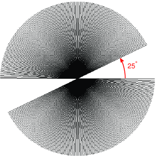
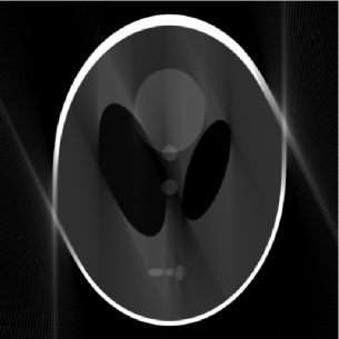
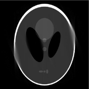
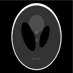
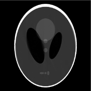
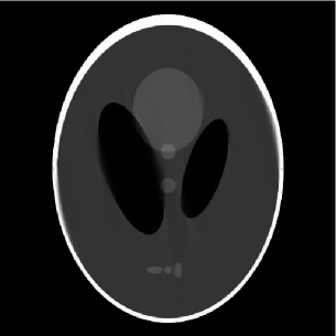
Figure 2: (a) $155$ limited-angle projections in the 2-D frequency plane, (b) the full and outer-shell masks of the Shepp-Logan phantom, (c) FBP ($\mbox{PSNR}=19.9$ dB), (d) DORE ($\mbox{PSNR}=22.7$ dB), (e) GPSR ($\mbox{PSNR}=22.9$ dB), (f) FPC${}_{\footnotesize\mbox{AS}}$ ($\mbox{PSNR}=22.5$ dB), (g) mask DORE ($\mbox{PSNR}=25.8$ dB), (h) mask GPSR ($\mbox{PSNR}=25.3$ dB), and (i) mask FPC${}_{\footnotesize\mbox{AS}}$ ($\mbox{PSNR}=26.4$ dB) reconstructions.

Shepp-Logan phantom reconstruction. We simulated limited-angle parallel-beam projections of an analog Shepp-Logan phantom with $1^{\circ}$ spacing between projections and missing angle span of $25^{\circ}$. Each projection is computed from its analytical sinogram using [8, function ellipse_sino.m] and [7] and then sampled by a receiver array containing $511$ elements. We then compute FFT of each projection, yielding $N=512$ frequency-domain measurements; the corresponding frequency-domain sampling pattern is shown in Fig. 2.

Fig. 2 depicts both the full and outer-shell masks of the phantom that we use to implement the DORE, GPSR, FPC${}_{\footnotesize\mbox{AS}}$ and mask DORE, GPSR, and FPC${}_{\footnotesize\mbox{AS}}$ methods, respectively. Because of the nature of X-ray CT measurements, our full mask has circular shape containing $p=205859$ signal elements. The elliptical outer-shell mask containing $p_{{\scriptstyle{\rm M}}}=130815\approx 0.6355\,p$ pixels has been constructed from the phantom’s sinogram using $\bigcap_{k=1}^{180}A_{\pi\,(k-1)/180}$, see Section V; this choice of the mask implies that we have prior information about the shape of the outer shell of the Shepp-Logan phantom beyond the information available from the limited-angle projections that we use for reconstruction, see Fig. 2.

Our performance metric is the peak signal-to-noise ratio (PSNR) of a reconstructed image $\widehat{\mbox{\boldmath$x$}}=[\widehat{x}_{1},\widehat{x}_{2},\ldots,\widehat{x}_{p}]^{T}$ inside the mask M:

$$\mbox{PSNR}~{}\mbox{(dB)}=10\,\log_{10}\Big{\{}\frac{[(\max_{i\in{\scriptstyle{\rm M}}}x_{i})-(\min_{i\in{\scriptstyle{\rm M}}}x_{i})]^{2}}{\sum_{i\in{\scriptstyle{\rm M}}}(\widehat{x}_{i}-x_{i})^{2}/p_{{\scriptstyle{\rm M}}}}\Big{\}}$$

where $x$ is the true image.

We select the inverse Haar (Daubechies-2) DWT matrix to be the orthogonal sparsifying transform matrix ${\mathit{\Psi}}$; the true signal vector $s$ consists of the Haar wavelet transform coefficients of the phantom and is sparse:

$$\|\mbox{\boldmath$s$}\|_{0}=7866\approx 0.0382\,p.$$

For the above choices of the mask and sparsifying transform, the number of identifiable signal transform coefficients is $p_{{\scriptstyle{\rm I}}}=132450\approx 0.6434\,p$. Note that $\|\mbox{\boldmath$s$}\|_{0}=\|\mbox{\boldmath$s$}_{{\scriptstyle{\rm I}}}\|_{0}\ll p_{{\scriptstyle{\rm I}}}$, implying that the identifiable signal coefficients are sparse as well.

We compare the reconstruction performances of

• mask DORE ($r=7000$) and DORE ($r=8000$) with $\epsilon=10^{-14}$ [see (16)], where $r$ are tuned for good PSNR performance;

• the mask FPC${}_{\footnotesize\mbox{AS}}$, mask GPSR, FPC${}_{\footnotesize\mbox{AS}}$, and GPSR schemes, all using the regularization parameter $\tau=10^{-5}\,\|H^{T}\,\mbox{\boldmath$y$}\|_{\infty}$ tuned for good PSNR performance;

• the standard FBP method.

(Here, we employ the convergence threshold $\texttt{tolP}=10^{-5}$ for the mask GPSR and GPSR schemes, see [6].)

Figs. 2–2 show the reconstructions of various methods. To facilitate comparison, we employ the common gray scale to represent the pixel values within the images in Figs. 2–2. Clearly, taking the object’s contour into account improves the signal reconstruction performance.

Industrial object reconstruction. We apply our proposed methods to reconstruct an industrial object from real fan-beam X-ray CT projections. First, we performed the standard fan-to-parallel beam conversion (see [7, Sec. 3.4]) and generated parallel-beam projections with $1^{\circ}$ spacing and measurement array size of $1023$ elements, yielding $N=1024$ frequency-domain measurements per projection. Our full mask has circular shape containing $p=823519$ signal elements. The outer-shell mask containing $p_{{\scriptstyle{\rm M}}}=529079\approx 0.6425\,p$ pixels has been constructed from the phantom’s parallel-beam sinogram using $\bigcap_{k=1}^{180}A_{\pi\,(k-1)/180}$, see Section V.

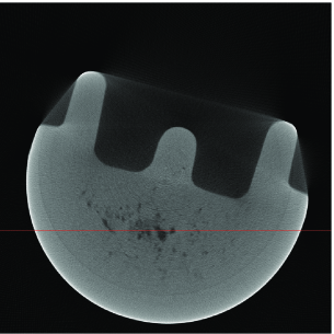
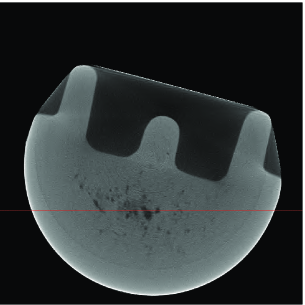
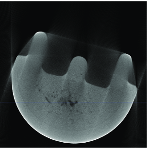
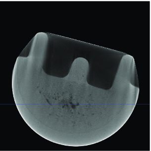
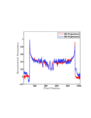
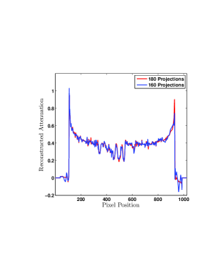
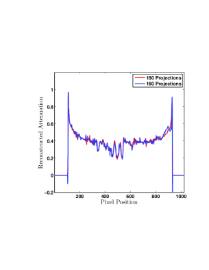
Figure 3: FBP, DORE, and mask DORE reconstructions from (a)–(c) $180$ projections and (d)–(f) $160$ limited-angle projections; (g)–(i) the corresponding FBP, DORE, and mask DORE reconstruction profiles for slices depicted in (a)–(f).

The $m\times m$ orthonormal sparsifying matrix ${\mathit{\Psi}}$ is constructed using the inverse Daubechies-6 DWT matrix.

We consider two measurement scenarios: no missing angles, i.e. all $180$ projections available, and limited-angle projections with missing angle span of $20^{\circ}$, i.e. $160$ projections available.

We compare the reconstruction performances of mask DORE ($r=15000$) and DORE ($r=20000$) with $\epsilon=10^{-8}$; the mask FPC${}_{\footnotesize\mbox{AS}}$ and FPC${}_{\footnotesize\mbox{AS}}$ schemes using the regularization parameter $\tau=10^{-6}\,\|H^{T}\,\mbox{\boldmath$y$}\|_{\infty}$; the standard FBP method. The reconstructions of mask FPC${}_{\footnotesize\mbox{AS}}$ and FPC${}_{\footnotesize\mbox{AS}}$ are very similar to those of mask DORE and DORE; hence we present only the mask DORE and DORE reconstructions in this example. Figs. 3–3 show the reconstructions of the FBP, DORE, and mask DORE methods from $180$ projections whereas Figs. 3–3 show the corresponding reconstructions from $160$ limited-angle projections. Figs. 3–3 show the corresponding reconstruction profiles for slices depicted in Figs. 3–3. Observe the aliasing correction and denoising achieved by the sparse reconstruction methods.

Appendix

We now prove Theorem 1. Consider the inequality:

$$\IEEEeqnarraymulticol{3}{l}{\|\mbox{\boldmath$y$}\kern-0.50003pt-\kern-0.50003ptH\mbox{\boldmath$s$}_{{\scriptstyle{\rm I}}}^{(q)}\|_{2}^{2}\kern-0.50003pt-\kern-0.50003pt\|\mbox{\boldmath$y$}\kern-0.50003pt-\kern-0.50003ptH\mbox{\boldmath$\widehat{s}$}_{{\scriptstyle{\rm I}}}\|_{2}^{2}\kern-0.50003pt=\kern-0.50003pt\|\mbox{\boldmath$y$}\kern-0.50003pt-\kern-0.50003ptH\mbox{\boldmath$s$}_{{\scriptstyle{\rm I}}}^{(q)}\|_{2}^{2}\kern-0.50003pt-\kern-0.50003pt\|\mbox{\boldmath$y$}\kern-0.50003pt-\kern-0.50003ptH\mbox{\boldmath$\widehat{s}$}_{{\scriptstyle{\rm I}}}\|_{2}^{2}}$$

$$+\>\frac{1}{\mu^{(q)}}\|\mbox{\boldmath$s$}_{{\scriptstyle{\rm I}}}^{(q)}-\mbox{\boldmath$s$}_{{\scriptstyle{\rm I}}}^{(q)}\|_{2}^{2}-\|H\,(\mbox{\boldmath$s$}_{{\scriptstyle{\rm I}}}^{(q)}-{\mbox{\boldmath$s$}_{{\scriptstyle{\rm I}}}}^{(q)})\|_{2}^{2}$$

$$\geq \|\mbox{\boldmath$y$}-H\,\mbox{\boldmath$\widehat{s}$}_{{\scriptstyle{\rm I}}}\|_{2}^{2}+\frac{1}{\mu^{(q)}}\|\mbox{\boldmath$\widehat{s}$}_{{\scriptstyle{\rm I}}}-{\mbox{\boldmath$s$}_{{\scriptstyle{\rm I}}}}^{(q)}\|_{2}^{2}-\|H\,(\mbox{\boldmath$\widehat{s}$}_{{\scriptstyle{\rm I}}}-{\mbox{\boldmath$s$}_{{\scriptstyle{\rm I}}}}^{(q)})\|_{2}^{2}$$

$$-\>\|\mbox{\boldmath$y$}-H\,\mbox{\boldmath$\widehat{s}$}_{{\scriptstyle{\rm I}}}\|_{2}^{2}$$

$$= \frac{1}{\mu^{(q)}}\,\|\mbox{\boldmath$\widehat{s}$}_{{\scriptstyle{\rm I}}}-{\mbox{\boldmath$s$}_{{\scriptstyle{\rm I}}}}^{(q)}\|_{2}^{2}-\|H(\mbox{\boldmath$\widehat{s}$}_{{\scriptstyle{\rm I}}}-\mbox{\boldmath$s$}_{{\scriptstyle{\rm I}}}^{(q)})\|_{2}^{2}$$

$$\geq (\frac{1}{\mu^{(q)}}-\rho_{{\scriptstyle{\it H}}}^{2})\,\|\mbox{\boldmath$\widehat{s}$}_{{\scriptstyle{\rm I}}}-\mbox{\boldmath$s$}_{{\scriptstyle{\rm I}}}^{(q)}\|_{2}^{2}$$ (A1b)

where (A1) follows by using the fact $\mbox{\boldmath$\widehat{s}$}_{{\scriptstyle{\rm I}}}$ in (8) minimizes

$$\mu^{(q)}\|\mbox{\boldmath$y$}-H\,\mbox{\boldmath$s$}_{{\scriptstyle{\rm I}}}\|_{2}^{2}+\|\mbox{\boldmath$s$}_{{\scriptstyle{\rm I}}}-{\mbox{\boldmath$s$}_{{\scriptstyle{\rm I}}}}^{(q)}\|_{2}^{2}-\mu^{(q)}\|H(\mbox{\boldmath$s$}_{{\scriptstyle{\rm I}}}-{\mbox{\boldmath$s$}_{{\scriptstyle{\rm I}}}}^{(q)})\|_{2}^{2}$$ (A2)

over all $\mbox{\boldmath$s$}_{{\scriptstyle{\rm I}}}\in{\cal S}_{r}$, see also (14). To see this, observe that (A2) can be written as

$$\|\mbox{\boldmath$s$}_{{\scriptstyle{\rm I}}}-\mbox{\boldmath$s$}_{{\scriptstyle{\rm I}}}^{(q)}-\mu^{(q)}\,H^{T}\,(\mbox{\boldmath$y$}-H\,\mbox{\boldmath$s$}_{{\scriptstyle{\rm I}}}^{(q)})\|_{2}^{2}+\mbox{const}$$ (A3)

where const denotes terms that are not functions of $\mbox{\boldmath$s$}_{{\scriptstyle{\rm I}}}$. Finally, (A1b) follows by using the Rayleigh-quotient property [9, Theorem 21.5.6]: $\|H\,(\mbox{\boldmath$\widehat{s}$}_{{\scriptstyle{\rm I}}}-{\mbox{\boldmath$s$}_{{\scriptstyle{\rm I}}}}^{(q)})\|_{2}^{2}/\|\mbox{\boldmath$\widehat{s}$}_{{\scriptstyle{\rm I}}}-{\mbox{\boldmath$s$}_{{\scriptstyle{\rm I}}}}^{(q)}\|_{2}^{2}\leq\rho_{{\scriptstyle{\it H}}}^{2}$. Therefore, in each iteration, $\|\mbox{\boldmath$y$}-H\,\mbox{\boldmath$s$}_{{\scriptstyle{\rm I}}}^{(q)}\|_{2}^{2}$ is guaranteed to not increase if the condition (13) holds. Since the sequence $\|\mbox{\boldmath$y$}-H\,\mbox{\boldmath$s$}_{{\scriptstyle{\rm I}}}^{(q)}\|_{2}^{2}$ is monotonically non-increasing and lower bounded by zero, it converges to a limit.

References

- [1] J. A. Tropp and S. J. Wright, “Computational methods for sparse solution of linear inverse problems,” Proc. IEEE, vol. 98, no. 6, pp. 948–958, 2010.
- [2] A. Manduca, J. D. Trzasko, and Z. Li, “Compressive sensing of images with a priori known spatial support,” in Medical Imaging 2010: Physics of Medical Imaging, ser. Proc. SPIE, E. Samei and N. J. Pelc, Eds., vol. 7622, Mar. 2010.
- [3] A. Dogandžić, R. Gu, and K. Qiu, “Algorithms for sparse X-ray CT image reconstruction of objects with known contour,” in Rev. Progress Quantitative Nondestructive Evaluation, ser. AIP Conf. Proc., D. O. Thompson and D. E. Chimenti, Eds., vol. 31, Melville, NY, 2012.
- [4] T. Blumensath and M. E. Davies, “Iterative hard thresholding for compressed sensing,” Appl. Comput. Harmon. Anal., vol. 27, no. 3, pp. 265–274, 2009.
- [5] Z. Wen, W. Yin, D. Goldfarb, and Y. Zhang, “A fast algorithm for sparse reconstruction based on shrinkage, subspace optimization, and continuation,” SIAM J. Sci. Comput., vol. 32, no. 4, pp. 1832–1857, 2010.
- [6] M. A. T. Figueiredo, R. D. Nowak, and S. J. Wright, “Gradient projection for sparse reconstruction: Application to compressed sensing and other inverse problems,” IEEE J. Select. Areas Signal Processing, vol. 1, no. 4, pp. 586–597, 2007.
- [7] A. C. Kak and M. Slaney, Principles of Computerized Tomographic Imaging. New York: IEEE Press, 1988.
- [8] J. Fessler. Image reconstruction toolbox. [Online]. Available: http://www.eecs.umich.edu/~fessler/code/
- [9] D. A. Harville, Matrix Algebra From a Statistician’s Perspective. New York: Springer-Verlag, 1997.