Optimal conditions for slow passive release of heparin-binding growth factors from an affinity-based delivery system

Abstract

We consider a mathematical model that describes the release of heparin-binding growth factors from an affinity-based delivery system. In the delivery system, heparin binds to a peptide which has been covalently cross-linked to a fibrin matrix. Growth factor in turn binds to the heparin, and growth factor release is governed by both binding and diffusion mechanisms, the purpose of the binding being to slow growth factor release. The governing mathematical model, which in its original formulation consists of five partial differential equations, is reduced to a system of just two equations. We identify the governing non-dimensional parameters that can be varied to tune the growth factor release rate. In particular, we identify a parameter regime that ensures slow passive release (usually desirable) of at least a fraction of the growth factor. It is found that slow release is assured if the matrix is prepared with the concentration of cross-linked peptide greatly exceeding the dissociation constant of heparin from the peptide, and with the concentration of heparin greatly exceeding the dissociation constant of the growth factor from heparin. Also, for the first time, in vitro experimental release data is directly compared with theoretical release profiles generated by the model. We propose that the two stage release behaviour frequently seen in experiments is due to an initial rapid out-diffusion of free growth factor over a diffusion time scale (typically days), followed by a much slower release of the bound fraction over a time scale depending on both diffusion and binding parameters (frequently months). drug delivery; heparin-binding growth factor; mathematical model.

1 Introduction

Background

In verterbrates, the extracellular matrix is a complex mixture of carbohydrates, proteins, and possibly minerals, that surrounds the cells that form tissues (Alberts et al. (2002)). The extracellular matrix helps cells to bind together, and regulates a number of cellular functions, such as differentiation, proliferation, migration, and adhesion. The matrix can achieve such regulation via the appropriate release of growth factors, for which it can act as a depot. Macromolecules within the structure of the matrix can bind growth factors with high affinity, enabling the matrix to serve as a growth factor reservoir. In response to changes in local physiological conditions (such as the occurrence of a wound, for example), cells may secrete enzymes that can release such growth factor depots from the matrix. This natural growth factor release mechanism has inspired the design of affinity-based drug delivery systems that mimic the retentive and protective properties of the extracellular matrix for growth factor. In this paper, we analyze a mathematical model that describes drug release from some such delivery systems, make recommendations as to how delivery system should be prepared, and, for the first time, compare the predictions of the model directly with experimental data.

The extracellular matrix consists predominantly of two classes of macromolecules: glycosaminoglycans, and fibrous proteins, such as collagen and fibronectin. Glycosaminoglycans are polysaccharide polymers that typically have a repeating unit consisting of two sugars. Heparin is glycosaminoglycan of the matrix that is known to bind with a number growth factors in vivo via electrostatic interactions, examples being basic fibroblast growth factor (bFGF), nerve growth factor (NGF), neurotrophin-3 (NT-3), and vascular endothelial growth factor (VEGF).

Affinity-based drug delivery systems

Sakiyama-Elbert & Hubbell (2000a) have developed a growth factor delivery system for wound healing that exploits heparin’s ability to bind electrostatically with growth factor. The various elements of their system are depicted schematically in Figure 1. The natural blood clotting matrix, fibrin, was chosen as the base material. Three dimensional fibrin hydrogel scaffolds were fabricated, into which invading cells could infiltrate, and release (via enzymatic processes) growth factor attached to the fibrin matrix. The growth factor attaches to the matrix via a bi-domain peptide bound to heparin, as we now explain. The peptide contains a domain which covalently cross-links to the fibrin matrix. However, the peptide also contains a domain that can bind to heparin, and such bound heparin can in turn bind to heparin-binding growth factor. Hence, growth factor attachment to the matrix is dependent on three distinct interactions, which we crudely represent by: (fibrin)–(peptide)–(heparin)–(growth factor).

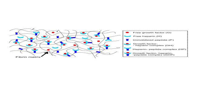
Figure 1: A schematic representation of the fibrin matrix containing all six species of the model.

The peptide is susceptible to cleavage by enzymes released from invading cells. Cells infiltrate the scaffold, release enzymes that degrade the peptide, and thereby release growth factor. In these systems, it is desirable that the growth factor be retained by the matrix until such time as it is actively released by cells. However, there inevitably will be some passive release, whereby free growth factor diffuses out of the system before cells have had the oppurtunity to actively release it. Growth factor binding to heparin is reversible, and it will not be permanently fixed to the matrix even in the absence of cells. The passive release of growth factor is usually undesirable, and in this study we use a mathematical model proposed by Sakiyama-Elbert & Hubbell (2000a) to help identify conditions that minimize it.

In Sakiyama-Elbert & Hubbell (2000a), the system was used to deliver the growth factor bFGF. Specifically, they carried out experiments in which they placed dorsal root ganglia from chickens in fibrin matrices loaded with bFGF. The purpose of their experiments was to evaluate the effect of the delivery system on neurite extension from the dorsal root ganglia. Their results demonstrated that the delivery system could enhance neurite extension by up to about 100% relative to unmodified fibrin. In subsequent studies, the system has been used to deliver NGF (Sakiyama-Elbert & Hubbell (2000b) and Wood et al. (2007, 2009)), NT-3 (Taylor et al. (2004) and Willerth et al. (2008)), glial-derived neurotrophic growth factor (GDNF) (Wood et al. (2008, 2009)), platelet-derived growth factor (PDGF) (Willerth et al. (2008)), and sonic hedgehog (Willerth et al. (2008)). In Wood et al. (2009), a 13 mm gap in a rat sciatic nerve was repaired using a silicone nerve guidance conduit containing the delivery system loaded with GDNF; a schematic representation of such a conduit is given in Figure 2.

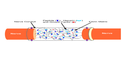
Figure 2: A schematic representation of a nerve guidance conduit containing the growth factor delivery system.

Matrix preparation

We identify which elements of the delivery system may be varied to tune growth factor release by briefly sketching how the fibrin matrices used in the above studies were prepared; see Sakiyama-Elbert & Hubbell (2000a) for the technical details and references. A fibrinogen solution was prepared by mixing the following components in appropriate quantity to achieve desired concentrations: plasminogen-free fibrinogen from pooled human plasma, calcium ions, thrombin, peptide, heparin, and growth factor. This polymerization mixture was placed in a well of a 24-well tissue culture plate and was incubated under appropriate conditions (Sakiyama-Elbert & Hubbell (2000a)) for an hour. It is clear then that the concentrations of the peptide, heparin and growth factor in the polymerization mixture are easily varied. However, a distinction needs to be made between the peptide that cross-links to the fibrin matrix and the peptide that remains unbound in the gel since it is the cross-linked peptide only that forms part of the delivery system. In Sakiyama et al. (1999) and Schense & Hubbell (1999), a procedure for quantifying the fraction of peptide that cross-links to the matrix is described. If the unbound peptide interacts significantly with the other free components of the system, then account must be taken of this in the mathematical modelling, and in Wood et al. (2007) a quite large mathematical model incorporating such effects is described. However, we do not incorporate free peptide in the model considered here for reasons we shall discuss in Section 3.

The system is complex

Lin & Metters (2006) comments that the mathematical model proposed by Sakiyama-Elbert & Hubbell (2000a) contains a relatively large number of parameters (we shall see that it has three diffusivities and four rate constants), and that this complicates their modelling approach. Indeed, the model in its original formulation does contain six differential equations, three of which contain diffusion terms. A major goal of the current study was to simplify the governing mathematical model. We shall show that under conditions of typical interest, the model can be reduced to a standard system of just two coupled partial differential equations governing the evolution of the concentrations of the total growth factor and total heparin. We shall further show that under typical conditions, the release behaviour is dominated by the values of just two non-dimensional parameters: the ratio of the concentration of cross-linked peptide to the dissociation constant of heparin from peptide, and the ratio of the initial concentration of heparin to the dissociation constant of the growth factor from heparin. Lin further comments that theoretical profiles generated by the model had yet to be directly compared with experimental data. We address this issue in Section 4.

2 Mathematical modelling

2.1 Model equations

The mathematical model which we shall now describe was first developed by Sakiyama-Elbert & Hubbell (2000a). There are six species in all in the model and, following Sakiyama-Elbert & Hubbell (2000a), we use the following notation:

$$P\mbox{ is an immobile peptide covalently fixed to the fibrin matrix;}$$

$$H\mbox{ is a mobile free heparin molecule that can diffuse through the fibrin matrix;}$$

$$G\mbox{ is a mobile free growth factor molecule that can diffuse through the fibrin matrix;}$$

$$GH\mbox{ is a mobile growth factor-heparin complex that can diffuse through the fibrin matrix;}$$

$$HP\mbox{ is an immobile heparin-peptide complex fixed to the fibrin matrix;}$$

$$GHP\mbox{ is an immobile growth factor-heparin-peptide complex fixed to the fibrin matrix.}$$

In Figure 1, we schematically represent all six species in the matrix. The possible interactions between these various species are described by the following four chemical reactions:

$$G+H\underset{{k_{\mbox{\tiny r}}}}{\overset{{k_{\mbox{\tiny f}}}}{\rightleftharpoons}}GH\hskip 34.14322ptG+HP\underset{{k_{\mbox{\tiny r}}}}{\overset{{k_{\mbox{\tiny f}}}}{\rightleftharpoons}}GHP$$

(2.1)

$$H+P\underset{{{\mbox{\tiny K}}_{\mbox{\tiny R}}}}{\overset{{{\mbox{\tiny K}}_{\mbox{\tiny F}}}}{\rightleftharpoons}}HP\hskip 34.14322ptGH+P\underset{{{\mbox{\tiny K}}_{\mbox{\tiny R}}}}{\overset{{{\mbox{\tiny K}}_{\mbox{\tiny F}}}}{\rightleftharpoons}}GHP$$

where $k_{f},k_{r},\kappa_{F},\kappa_{R}$ are the rate constants as shown. The first reaction, for example, represents the reversible binding of a free growth factor molecule to a free heparin molecule, with association and dissociation rate constants $k_{f}$ and $k_{r}$, respectively. The other three reactions are similarly interpreted; see Figure 1. It is noteworthy that we have assumed that the rate constants for the first and second reactions above are the same, and similarly for the third and fourth reactions. This implies that we are assuming that the association/dissociation behaviour of growth factor for heparin does not depend on whether the heparin is free or bound to peptide; a similar comment applies to the binding heparin to peptide.

The problems that are considered in this paper are one-dimensional, and throughout we shall denote the spatial variable by $x$ and the time variable by $t$. Following the notation of Sakiyama-Elbert & Hubbell (2000a), we denote by $c_{\mbox{\tiny G}}(x,t)$ the concentration of free growth factor $G$ at location $x$ and time $t$; the notation for the concentrations of the other five species follows in an obvious fashion. In view of the chemical reactions (2.1), and our assumptions regarding the mobility of the various species, the governing equations for the six concentrations take the form:

$$\frac{\partial c_{\mbox{\tiny G}}}{\partial t}=D_{\mbox{\tiny G}}\frac{\partial^{2}c_{\mbox{\tiny G}}}{\partial x^{2}}-k_{f}c_{\mbox{\tiny G}}c_{\mbox{\tiny H}}+k_{r}c_{\mbox{\tiny GH}}-k_{f}c_{\mbox{\tiny G}}c_{\mbox{\tiny HP}}+k_{r}c_{\mbox{\tiny GHP}},$$

$$\frac{\partial c_{\mbox{\tiny H}}}{\partial t}=D_{\mbox{\tiny H}}\frac{\partial^{2}c_{\mbox{\tiny H}}}{\partial x^{2}}-k_{f}c_{\mbox{\tiny G}}c_{\mbox{\tiny H}}+k_{r}c_{\mbox{\tiny GH}}-{\mbox{\tiny K}}_{\mbox{\tiny F}}c_{\mbox{\tiny H}}c_{\mbox{\tiny P}}+{\mbox{\tiny K}}_{\mbox{\tiny R}}c_{\mbox{\tiny HP}},$$

$$\frac{\partial c_{\mbox{\tiny GH}}}{\partial t}=D_{\mbox{\tiny GH}}\frac{\partial^{2}c_{\mbox{\tiny GH}}}{\partial x^{2}}+k_{f}c_{\mbox{\tiny G}}c_{\mbox{\tiny H}}-k_{r}c_{\mbox{\tiny GH}}-{\mbox{\tiny K}}_{\mbox{\tiny F}}c_{\mbox{\tiny GH}}c_{\mbox{\tiny P}}+{\mbox{\tiny K}}_{\mbox{\tiny R}}c_{\mbox{\tiny GHP}},$$ (2.2)

$$\frac{\partial c_{\mbox{\tiny P}}}{\partial t}=-{\mbox{\tiny K}}_{\mbox{\tiny F}}c_{\mbox{\tiny H}}c_{\mbox{\tiny P}}+{\mbox{\tiny K}}_{\mbox{\tiny R}}c_{\mbox{\tiny HP}}-{\mbox{\tiny K}}_{\mbox{\tiny F}}c_{\mbox{\tiny GH}}c_{\mbox{\tiny P}}+{\mbox{\tiny K}}_{\mbox{\tiny R}}c_{\mbox{\tiny GHP}},$$

$$\frac{\partial c_{\mbox{\tiny HP}}}{\partial t}=-k_{f}c_{\mbox{\tiny G}}c_{\mbox{\tiny HP}}+k_{r}c_{\mbox{\tiny GHP}}+{\mbox{\tiny K}}_{\mbox{\tiny F}}c_{\mbox{\tiny H}}c_{\mbox{\tiny P}}-{\mbox{\tiny K}}_{\mbox{\tiny R}}c_{\mbox{\tiny HP}},$$

$$\frac{\partial c_{\mbox{\tiny GHP}}}{\partial t}=k_{f}c_{\mbox{\tiny G}}c_{\mbox{\tiny HP}}-k_{r}c_{\mbox{\tiny GHP}}+{\mbox{\tiny K}}_{\mbox{\tiny F}}c_{\mbox{\tiny GH}}c_{\mbox{\tiny P}}-{\mbox{\tiny K}}_{\mbox{\tiny R}}c_{\mbox{\tiny GHP}},$$

where $D_{\mbox{\tiny G}}$, $D_{\mbox{\tiny H}}$ and $D_{\mbox{\tiny GH}}$ are the diffusivities for the free growth factor, free heparin, and free growth factor-heparin complex, respectively; the species $P$, $HP$ and $GHP$ are taken to be immobile since the peptide is assumed to be covalently fixed to the fibrin matrix, and consequently the equations for their concentrations do not contain diffusion terms.

2.2 Boundary and initial conditions

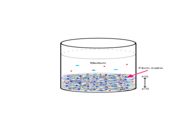
Figure 3: A schematic depiction of the experimental setup for the release of growth factor from the fibrin matrix.

We choose simple boundary conditions for (2.2) that allow direct comparison with available experimental and theoretical results for growth factor release from the delivery system. We suppose that the fibrin matrix occupies $0\leq x\leq L$, with $x=0$ giving the location of a container wall through which the growth factor cannot penetrate, and $x=L$ denoting the interface between the matrix and an external medium into which growth factor releases; see Figure 3. At the container wall, we impose no-flux conditions for the mobile species, so that:

$$\frac{\partial c_{\mbox{\tiny G}}}{\partial x}=0,\hskip 5.69046pt\frac{\partial c_{\mbox{\tiny H}}}{\partial x}=0,\hskip 5.69046pt\frac{\partial c_{\mbox{\tiny GH}}}{\partial x}=0\hskip 11.38092pt\mbox{ on }x=0.$$ (2.3)

At the interface between the matrix and the external medium, we impose perfect sink conditions for the mobile species:

$$c_{\mbox{\tiny G}}=0,\hskip 5.69046ptc_{\mbox{\tiny H}}=0,\hskip 5.69046ptc_{\mbox{\tiny GH}}=0\hskip 11.38092pt\mbox{ on }x=L.$$ (2.4)

The boundary conditions (2.3), (2.4) could also model in-vitro growth factor release from a nerve guide tube (Sakiyama-Elbert & Hubbell (2000a)) occupying $-L\leq x\leq L$, with $x=\pm L$ giving the location of the ends of the tube; see Figure 2. In this context, (2.3) are interpreted as symmetry conditions on the centre-line of the tube.

Equations (2.2) are solved subject to the following initial conditions:

$$c_{\mbox{\tiny G}}=c_{\mbox{\tiny G}}^{\mbox{\tiny 0}},\hskip 5.69046ptc_{\mbox{\tiny H}}=c_{\mbox{\tiny H}}^{\mbox{\tiny 0}},\hskip 5.69046ptc_{\mbox{\tiny GH}}=0,\hskip 5.69046ptc_{\mbox{\tiny P}}=c_{\mbox{\tiny P}}^{\mbox{\tiny 0}},\hskip 5.69046ptc_{\mbox{\tiny HP}}=0,\hskip 5.69046ptc_{\mbox{\tiny GHP}}=0\hskip 11.38092pt\mbox{ at }t=0,$$ (2.5)

where $c_{\mbox{\tiny G}}^{\mbox{\tiny 0}},c_{\mbox{\tiny H}}^{\mbox{\tiny 0}},c_{\mbox{\tiny P}}^{\mbox{\tiny 0}}$ denote the initial concentrations of growth factor, heparin, and peptide, respectively, in the polymerization mixture. In our modelling, we make the simplifying assumption that all of the peptide in the polymerization mixture crosslinks covalently to the fibrin matrix. This is not likely to occur in practice, but we shall show in Section 3 how our results may be modified to take account of the presence of free peptide in the matrix. It should also be noted that free peptide will typically clear the system over a period of a few days. We conclude this section by emphasising that the key results of this paper are quite general for the model under typical conditions, and are not strongly dependent on the particular choice of boundary and initial conditions made.

The mathematical model is now complete, and consists of equations (2.2), (2.3), (2.4), (2.5).

2.3 Model reduction

We now show how the model may frequently be reduced to a coupled pair of partial differential equations.

2.3.1 Non-dimensionalisation

Before giving the non-dimensionalisation, we first note that (2.2) may be written in the following equivalent form:

$$\frac{\partial}{\partial t}({c_{\mbox{\tiny G}}+c_{\mbox{\tiny GH}}+c_{\mbox{\tiny GHP}}})=D_{\mbox{\tiny G}}\frac{\partial^{2}c_{\mbox{\tiny G}}}{\partial x^{2}}+D_{\mbox{\tiny GH}}\frac{\partial^{2}c_{\mbox{\tiny GH}}}{\partial x^{2}},$$

$$\frac{\partial}{\partial t}\left(c_{\mbox{\tiny H}}+c_{\mbox{\tiny GH}}+c_{\mbox{\tiny HP}}+c_{\mbox{\tiny GHP}}\right)=D_{\mbox{\tiny H}}\frac{\partial^{2}c_{\mbox{\tiny H}}}{\partial x^{2}}+D_{\mbox{\tiny GH}}\frac{\partial^{2}c_{\mbox{\tiny GH}}}{\partial x^{2}},$$

$$\frac{\partial}{\partial t}({c_{\mbox{\tiny GH}}+c_{\mbox{\tiny GHP}}})=D_{\mbox{\tiny GH}}\frac{\partial^{2}c_{\mbox{\tiny GH}}}{\partial x^{2}}+k_{f}c_{\mbox{\tiny G}}(c_{\mbox{\tiny H}}+c_{\mbox{\tiny HP}})-k_{r}(c_{\mbox{\tiny GH}}+c_{\mbox{\tiny GHP}}),$$ (2.6)

$$\frac{\partial}{\partial t}\left(c_{\mbox{\tiny HP}}+c_{\mbox{\tiny GHP}}\right)={\mbox{\tiny K}}_{\mbox{\tiny F}}c_{\mbox{\tiny P}}\left(c_{\mbox{\tiny H}}+c_{\mbox{\tiny GH}}\right)-{\mbox{\tiny K}}_{\mbox{\tiny R}}\left(c_{\mbox{\tiny HP}}+c_{\mbox{\tiny GHP}}\right),$$

$$\frac{\partial c_{\mbox{\tiny GHP}}}{\partial t}=k_{f}c_{\mbox{\tiny G}}c_{\mbox{\tiny HP}}+{\mbox{\tiny K}}_{\mbox{\tiny F}}c_{\mbox{\tiny GH}}c_{\mbox{\tiny P}}-(k_{r}+{\mbox{\tiny K}}_{\mbox{\tiny R}})c_{\mbox{\tiny GHP}},$$

$$c_{\mbox{\tiny P}}+c_{\mbox{\tiny HP}}+c_{\mbox{\tiny GHP}}=c_{\mbox{\tiny P}}^{\mbox{\tiny 0}},$$

where, for example, equation (2.6)₆ is obtained by forming (2.2)₄+ (2.2)₅+ (2.2)₆. We denote the total concentrations of growth factor and heparin in the matrix by $c_{\mbox{\tiny G}}^{\mbox{\tiny T}}$ and $c_{\mbox{\tiny H}}^{\mbox{\tiny T}}$, respectively, so that:

$$c_{\mbox{\tiny G}}^{\mbox{\tiny T}}=c_{\mbox{\tiny G}}+c_{\mbox{\tiny GH}}+c_{\mbox{\tiny GHP}},\hskip 5.69046ptc_{\mbox{\tiny H}}^{\mbox{\tiny T}}=c_{\mbox{\tiny H}}+c_{\mbox{\tiny GH}}+c_{\mbox{\tiny HP}}+c_{\mbox{\tiny GHP}}.$$ (2.7)

Equations (2.6)₁ and (2.6)₂ give the evolution equations for the total growth factor and heparin, and may be written in conservation form as:

$$\frac{\partial c_{\mbox{\tiny G}}^{\mbox{\tiny T}}}{\partial t}+\frac{\partial j_{\mbox{\tiny G}}^{\mbox{\tiny T}}}{\partial x}=0,\hskip 8.5359pt\frac{\partial c_{\mbox{\tiny H}}^{\mbox{\tiny T}}}{\partial t}+\frac{\partial j_{\mbox{\tiny H}}^{\mbox{\tiny T}}}{\partial x}=0,$$ (2.8)

where

$$j_{\mbox{\tiny G}}^{\mbox{\tiny T}}=-D_{\mbox{\tiny G}}\frac{\partial c_{\mbox{\tiny G}}}{\partial x}-D_{\mbox{\tiny GH}}\frac{\partial c_{\mbox{\tiny GH}}}{\partial x},\hskip 8.5359ptj_{\mbox{\tiny H}}^{\mbox{\tiny T}}=-D_{\mbox{\tiny H}}\frac{\partial c_{\mbox{\tiny H}}}{\partial x}-D_{\mbox{\tiny GH}}\frac{\partial c_{\mbox{\tiny GH}}}{\partial x},$$ (2.9)

give the total flux of growth factor and heparin, respectively.

We introduce non-dimensional variables as follows:

$$\bar{x}=\frac{x}{L},\hskip 5.69046pt\bar{t}=\frac{t}{(L^{2}/D_{\mbox{\tiny GH}})},\hskip 5.69046pt\bar{c}_{\mbox{\tiny G}}=\frac{c_{\mbox{\tiny G}}}{c_{\mbox{\tiny G}}^{\mbox{\tiny 0}}},\hskip 5.69046pt\bar{c}_{\mbox{\tiny H}}=\frac{c_{\mbox{\tiny H}}}{c_{\mbox{\tiny H}}^{\mbox{\tiny 0}}},\hskip 5.69046pt\bar{c}_{\mbox{\tiny P}}=\frac{c_{\mbox{\tiny P}}}{c_{\mbox{\tiny P}}^{\mbox{\tiny 0}}},\hskip 5.69046pt\bar{c}_{\mbox{\tiny GH}}=\frac{c_{\mbox{\tiny GH}}}{c_{\mbox{\tiny G}}^{\mbox{\tiny 0}}},$$

$$\bar{c}_{\mbox{\tiny GHP}}=\frac{c_{\mbox{\tiny GHP}}}{c_{\mbox{\tiny G}}^{\mbox{\tiny 0}}},\hskip 5.69046pt\bar{c}_{\mbox{\tiny HP}}=\frac{c_{\mbox{\tiny HP}}}{c_{\mbox{\tiny H}}^{\mbox{\tiny 0}}},\hskip 5.69046pt\bar{c}_{\mbox{\tiny G}}^{\mbox{\tiny T}}=\frac{c_{\mbox{\tiny G}}^{\mbox{\tiny T}}}{c_{\mbox{\tiny G}}^{\mbox{\tiny 0}}},\hskip 5.69046pt\bar{c}_{\mbox{\tiny H}}^{\mbox{\tiny T}}=\frac{c_{\mbox{\tiny H}}^{\mbox{\tiny T}}}{c_{\mbox{\tiny H}}^{\mbox{\tiny 0}}},\hskip 5.69046pt\bar{j}_{\mbox{\tiny G}}^{\mbox{\tiny T}}=\frac{j_{\mbox{\tiny G}}^{\mbox{\tiny T}}}{(D_{\mbox{\tiny GH}}c_{\mbox{\tiny G}}^{\mbox{\tiny 0}}/L)},\hskip 5.69046pt\bar{j}_{\mbox{\tiny H}}^{\mbox{\tiny T}}=\frac{j_{\mbox{\tiny H}}^{\mbox{\tiny T}}}{(D_{\mbox{\tiny GH}}c_{\mbox{\tiny H}}^{\mbox{\tiny 0}}/L)},$$

to obtain the following non-dimensional form for the governing initial boundary value problem (upon dropping over-bars):

$$\frac{\partial}{\partial t}({c_{\mbox{\tiny G}}+c_{\mbox{\tiny GH}}+c_{\mbox{\tiny GHP}}})=D_{\mbox{\tiny G}}^{*}\frac{\partial^{2}c_{\mbox{\tiny G}}}{\partial x^{2}}+\frac{\partial^{2}c_{\mbox{\tiny GH}}}{\partial x^{2}},$$

$$\frac{\partial}{\partial t}\left(c_{\mbox{\tiny H}}+c_{\mbox{\tiny HP}}+(c_{\mbox{\tiny GH}}+c_{\mbox{\tiny GHP}})/\eta_{\mbox{\tiny H/G}}\right)=D_{\mbox{\tiny H}}^{*}\frac{\partial^{2}c_{\mbox{\tiny H}}}{\partial x^{2}}+\frac{1}{\eta_{\mbox{\tiny H/G}}}\frac{\partial^{2}c_{\mbox{\tiny GH}}}{\partial x^{2}},$$

$$\delta_{\mbox{\tiny G}}\frac{\partial}{\partial t}({c_{\mbox{\tiny GH}}+c_{\mbox{\tiny GHP}}})=\delta_{\mbox{\tiny G}}\frac{\partial^{2}c_{\mbox{\tiny GH}}}{\partial x^{2}}+K_{b\mbox{\tiny H}}c_{\mbox{\tiny G}}(c_{\mbox{\tiny H}}+c_{\mbox{\tiny HP}})-(c_{\mbox{\tiny GH}}+c_{\mbox{\tiny GHP}}),$$

$$\delta_{\mbox{\tiny H}}\frac{\partial}{\partial t}\left(\eta_{\mbox{\tiny H/G}}c_{\mbox{\tiny HP}}+c_{\mbox{\tiny GHP}}\right)=K_{b\mbox{\tiny P}}c_{\mbox{\tiny P}}\left(\eta_{\mbox{\tiny H/G}}c_{\mbox{\tiny H}}+c_{\mbox{\tiny GH}}\right)-\left(\eta_{\mbox{\tiny H/G}}c_{\mbox{\tiny HP}}+c_{\mbox{\tiny GHP}}\right),$$ (2.10)

$$\delta_{\mbox{\tiny G}}\delta_{\mbox{\tiny H}}\frac{\partial c_{\mbox{\tiny GHP}}}{\partial t}=\delta_{\mbox{\tiny H}}(K_{b\mbox{\tiny H}}c_{\mbox{\tiny G}}c_{\mbox{\tiny HP}}-c_{\mbox{\tiny GHP}})+\delta_{\mbox{\tiny G}}(K_{b\mbox{\tiny P}}c_{\mbox{\tiny GH}}c_{\mbox{\tiny P}}-c_{\mbox{\tiny GHP}}),$$

$$c_{\mbox{\tiny P}}+\eta_{\mbox{\tiny H/P}}c_{\mbox{\tiny HP}}+\frac{\eta_{\mbox{\tiny H/P}}}{\eta_{\mbox{\tiny H/G}}}c_{\mbox{\tiny GHP}}=1,$$

$$\frac{\partial c_{\mbox{\tiny G}}}{\partial x}=0,\hskip 5.69046pt\frac{\partial c_{\mbox{\tiny H}}}{\partial x}=0,\hskip 5.69046pt\frac{\partial c_{\mbox{\tiny GH}}}{\partial x}=0\hskip 5.69046pt\mbox{ on }x=0,$$

$$c_{\mbox{\tiny G}}=0,\hskip 5.69046ptc_{\mbox{\tiny H}}=0,\hskip 5.69046ptc_{\mbox{\tiny GH}}=0\hskip 5.69046pt\mbox{ on }x=1,$$

$$c_{\mbox{\tiny G}}=1,\hskip 5.69046ptc_{\mbox{\tiny H}}=1,\hskip 5.69046ptc_{\mbox{\tiny GH}}=0,\hskip 5.69046ptc_{\mbox{\tiny P}}=1,\hskip 5.69046ptc_{\mbox{\tiny HP}}=0,\hskip 5.69046ptc_{\mbox{\tiny GHP}}=0\hskip 5.69046pt\mbox{ at }t=0,$$

where:

$$D_{\mbox{\tiny G}}^{*}=\frac{D_{\mbox{\tiny G}}}{D_{\mbox{\tiny GH}}},\hskip 5.69046ptD_{\mbox{\tiny H}}^{*}=\frac{D_{\mbox{\tiny H}}}{D_{\mbox{\tiny GH}}},\hskip 5.69046pt\eta_{\mbox{\tiny H/G}}=\frac{c_{\mbox{\tiny H}}^{\mbox{\tiny 0}}}{c_{\mbox{\tiny G}}^{\mbox{\tiny 0}}},\hskip 5.69046pt\eta_{\mbox{\tiny H/P}}=\frac{c_{\mbox{\tiny H}}^{\mbox{\tiny 0}}}{c_{\mbox{\tiny P}}^{\mbox{\tiny 0}}},$$

(2.11)

$$\delta_{\mbox{\tiny G}}=\frac{D_{\mbox{\tiny GH}}}{k_{r}L^{2}},\hskip 5.69046pt\delta_{\mbox{\tiny H}}=\frac{D_{\mbox{\tiny GH}}}{{\mbox{\tiny K}}_{\mbox{\tiny R}}L^{2}},\hskip 5.69046ptK_{b{\mbox{\tiny H}}}=\frac{k_{f}c_{\mbox{\tiny H}}^{\mbox{\tiny 0}}}{k_{r}},\hskip 5.69046ptK_{b{\mbox{\tiny P}}}=\frac{{\mbox{\tiny K}}_{\mbox{\tiny F}}c_{\mbox{\tiny P}}^{\mbox{\tiny 0}}}{{\mbox{\tiny K}}_{\mbox{\tiny R}}},$$

are the governing non-dimensional parameters. The quantities $K_{b{\mbox{\tiny H}}},K_{b{\mbox{\tiny P}}}$ give a non-dimensional measure of the strength of retention of growth factor by the heparin, and of heparin by the peptide, respectively. We denote by

$$K_{\mbox{\tiny G-H}}^{\mbox{\tiny D}}=\frac{k_{r}}{k_{f}},\hskip 5.69046ptK_{\mbox{\tiny H-P}}^{\mbox{\tiny D}}=\frac{{\mbox{\tiny K}}_{\mbox{\tiny R}}}{{\mbox{\tiny K}}_{\mbox{\tiny F}}},$$

the dissociation constants of growth factor from heparin, and of heparin from peptide, respectively, so that:

$$K_{b{\mbox{\tiny H}}}=\frac{c_{\mbox{\tiny H}}^{\mbox{\tiny 0}}}{K_{\mbox{\tiny G-H}}^{\mbox{\tiny D}}},\hskip 5.69046ptK_{b{\mbox{\tiny P}}}=\frac{c_{\mbox{\tiny P}}^{\mbox{\tiny 0}}}{K_{\mbox{\tiny H-P}}^{\mbox{\tiny D}}}.$$ (2.12)

It is noteworthy that $K_{b{\mbox{\tiny H}}}$ involves both the concentration of available binding sites for the growth factor and the dissociation constant of growth factor from heparin. The case $K_{b{\mbox{\tiny H}}}\gg 1$ corresponds to the growth factor being strongly retained by the heparin. Conversely, $K_{b{\mbox{\tiny H}}}\ll 1$ corresponds to weak retention of growth factor by the heparin. The parameter $K_{b{\mbox{\tiny P}}}$ is similarly interpreted in the context of heparin retention by the peptide.

The non-dimensional form for the total growth factor and heparin and their fluxes are given by:

$$c_{\mbox{\tiny G}}^{\mbox{\tiny T}}=c_{\mbox{\tiny G}}+c_{\mbox{\tiny GH}}+c_{\mbox{\tiny GHP}},\hskip 14.22636ptc_{\mbox{\tiny H}}^{\mbox{\tiny T}}=c_{\mbox{\tiny H}}+c_{\mbox{\tiny HP}}+(c_{\mbox{\tiny GH}}+c_{\mbox{\tiny GHP}})/\eta_{\mbox{\tiny H/G}},$$

(2.13)

$$j_{\mbox{\tiny G}}^{\mbox{\tiny T}}=-D_{\mbox{\tiny G}}^{*}\frac{\partial c_{\mbox{\tiny G}}}{\partial x}-\frac{\partial c_{\mbox{\tiny GH}}}{\partial x},\hskip 14.22636ptj_{\mbox{\tiny H}}^{\mbox{\tiny T}}=-D_{\mbox{\tiny H}}^{*}\frac{\partial c_{\mbox{\tiny H}}}{\partial x}-\frac{1}{\eta_{\mbox{\tiny H/G}}}\frac{\partial c_{\mbox{\tiny GH}}}{\partial x}.$$

2.3.2 Parameter values

In Sakiyama-Elbert & Hubbell (2000a); Taylor et al. (2004); Willerth et al. (2006, 2008) and Wood et al. (2007, 2008), the fibrin gels were prepared by placing 400 $\mu$l of polymerization mixture in the wells of a 24-well plate. The diameter of each well in such a plate is 1.56 cm, from which it follows that the thickness of the gels was $L\approx 0.2$ cm. In Sakiyama-Elbert & Hubbell (2000a), the heparin diffusivity was taken to be $D_{\mbox{\tiny H}}=3.13\times 10^{-5}$ cm²min^-1, and for bFGF, the diffusivities $D_{\mbox{\tiny G}}=6.0\times 10^{-5}$ cm²min^-1 and $D_{\mbox{\tiny GH}}=1.0\times 10^{-5}$ cm²min^-1 were used. These values, which were based on the work of Saltzman et al. (1994) and Gaigalas et al. (1995), all have order of magnitude $10^{-5}$ cm²min^-1. In Taylor et al. (2004), where the growth factor being considered was NT-3, the diffusivities used were again of order $10^{-5}$ cm²min^-1. Taking $D=3.0\times 10^{-5}$ cm²min^-1 as a representative diffusivity for a free species in the matrix and $L=0.2$ cm, we calculate a typical diffusion time scale for the system to be $L^{2}/D\approx 1$ day. Hence, in a release experiment where the diffusivities are of order $10^{-5}$ cm²min^-1, we would typically expect the unbound components to clear the system over a period of some days, and this is consistent with the experimental results of Taylor et al. (2004) and Wood et al. (2007, 2008).

There are also time scales associated with the rate constants for the chemical reactions (2.1), namely, $1/k_{r}$, $1/(k_{f}c_{\mbox{\tiny H}}^{\mbox{\tiny 0}})$, $1/\mbox{\tiny K}_{\mbox{\tiny R}}$, and $1/({\mbox{\tiny K}}_{\mbox{\tiny F}}c_{\mbox{\tiny P}}^{\mbox{\tiny 0}})$. In Sakiyama-Elbert & Hubbell (2000a) and Taylor et al. (2004), the values of the rate constants for the binding of heparin to the peptide were taken to be $\mbox{\tiny K}_{\mbox{\tiny R}}\approx 80$ min^-1 and $\mbox{\tiny K}_{\mbox{\tiny F}}\approx 10^{9}$ M^-1 min^-1, and $c_{\mbox{\tiny P}}^{\mbox{\tiny 0}}$ was of order $10^{-4}$ M. For these values, we find that $1/\mbox{\tiny K}_{\mbox{\tiny R}}\approx 1$ s, $1/({\mbox{\tiny K}}_{\mbox{\tiny F}}c_{\mbox{\tiny P}}^{\mbox{\tiny 0}})=10^{-5}$ s, and we note that these times are tiny compared to the typical time scales associated with diffusion (days), and furthermore, would remain so even if we made $c_{\mbox{\tiny P}}^{\mbox{\tiny 0}}$ orders of magnitude smaller. For the binding of growth factor to heparin, the rate constants will depend on the nature of the growth factor, and data is unfortunately frequently lacking. For bFGF, Sakiyama-Elbert & Hubbell (2000a) use the values $k_{r}\approx 1$ min^-1, $k_{f}\approx 10^{8}$ M^-1 min^-1, and take $c_{\mbox{\tiny H}}^{\mbox{\tiny 0}}\approx 6\times 10^{-5}$ M. For these values, $1/k_{r}=1$ min and $1/(k_{f}c_{\mbox{\tiny H}}^{\mbox{\tiny 0}})\approx 10^{-2}$ s, and these times are also small compared to the diffusion time scales.

For NT-3, the $k_{f}$ and $k_{r}$ values are unknown, but Taylor et al. (2004) gives the approximation $K_{D}^{\mbox{\tiny G-H}}\approx 10^{-6}$ M for the dissociation constant, which would imply that NT-3 has a low affinity for the heparin binding site. By contrast, bFGF has a relatively high affinity for the heparin binding site, with dissociation constant $K_{D}^{\mbox{\tiny G-H}}\approx 10^{-8}$ M. However, we shall show in this paper that, provided the governing mathematical model is appropriate, slow passive growth factor release is achieveable even for low affinity binding of growth factor to heparin.

2.3.3 Reduction to a pair of coupled partial differential equations

We conclude from the remarks above that for many systems of practical interest, the time scales for the association and dissociation rates in the chemical reactions (2.1) are much shorter than the diffusion time scales, so that we frequently have:

$$\frac{L^{2}}{D_{\mbox{\tiny G}}},\hskip 5.69046pt\frac{L^{2}}{D_{\mbox{\tiny H}}},\hskip 5.69046pt\frac{L^{2}}{D_{\mbox{\tiny GH}}}\gg\frac{1}{k_{r}},\hskip 5.69046pt\frac{1}{k_{f}c_{\mbox{\tiny H}}^{\mbox{\tiny 0}}},\hskip 5.69046pt\frac{1}{{\mbox{\tiny K}}_{\mbox{\tiny R}}},\hskip 5.69046pt\frac{1}{{\mbox{\tiny K}}_{\mbox{\tiny F}}c_{\mbox{\tiny P}}^{\mbox{\tiny 0}}}.$$

In such cases, diffusion is rate limiting since it is the slowest process. We restrict our attention to such systems in the current analysis. In terms of the dimensionless parameters (2.11), the conditions above imply that $\delta{\mbox{\tiny G}}\ll\min(K_{b{\mbox{\tiny H}}},1)$ and $\delta{\mbox{\tiny H}}\ll\min(K_{b{\mbox{\tiny P}}},1)$, and so the differential equations (2.10)₃, (2.10)₄ and (2.10)₅ are replaced by the algebraic expressions:

$$K_{b\mbox{\tiny H}}c_{\mbox{\tiny G}}(c_{\mbox{\tiny H}}+c_{\mbox{\tiny HP}})=c_{\mbox{\tiny GH}}+c_{\mbox{\tiny GHP}},\hskip 5.69046ptK_{b\mbox{\tiny P}}c_{\mbox{\tiny P}}\left(\eta_{\mbox{\tiny H/G}}c_{\mbox{\tiny H}}+c_{\mbox{\tiny GH}}\right)=\eta_{\mbox{\tiny H/G}}c_{\mbox{\tiny HP}}+c_{\mbox{\tiny GHP}},$$ (2.14)

$$\theta(K_{b\mbox{\tiny H}}c_{\mbox{\tiny G}}c_{\mbox{\tiny HP}}-c_{\mbox{\tiny GHP}})+K_{b\mbox{\tiny P}}c_{\mbox{\tiny GH}}c_{\mbox{\tiny P}}-c_{\mbox{\tiny GHP}}=0,$$

where $\theta=\delta{\mbox{\tiny H}}/\delta{\mbox{\tiny G}}=k_{r}/{\mbox{\tiny K}}_{\mbox{\tiny R}}$. The first two equations in (2.14) correspond to the equilibrium forms for the binding of growth factor to heparin, and of heparin to peptide, respectively.

We solve the six algebraic expressions (2.10)₆, (2.13)₁, (2.14) for the concentrations of the six species $c_{\mbox{\tiny G}}$, $c_{\mbox{\tiny H}}$, $c_{\mbox{\tiny GH}}$, $c_{\mbox{\tiny P}}$, $c_{\mbox{\tiny HP}}$, $c_{\mbox{\tiny GHP}}$ in terms of the total concentration of growth factor, $c_{\mbox{\tiny G}}^{\mbox{\tiny T}}$, and heparin, $c_{\mbox{\tiny H}}^{\mbox{\tiny T}}$, to obtain expressions of the form:

$$c_{\mbox{\tiny G}}=c_{\mbox{\tiny G}}(c_{\mbox{\tiny G}}^{\mbox{\tiny T}},c_{\mbox{\tiny H}}^{\mbox{\tiny T}}),\hskip 5.69046ptc_{\mbox{\tiny P}}=c_{\mbox{\tiny P}}(c_{\mbox{\tiny H}}^{\mbox{\tiny T}}),\hskip 5.69046ptc_{\mbox{\tiny GH}}=c_{\mbox{\tiny GH}}(c_{\mbox{\tiny G}}^{\mbox{\tiny T}},c_{\mbox{\tiny H}}^{\mbox{\tiny T}}),\hskip 5.69046ptc_{\mbox{\tiny GHP}}=c_{\mbox{\tiny GHP}}(c_{\mbox{\tiny G}}^{\mbox{\tiny T}},c_{\mbox{\tiny H}}^{\mbox{\tiny T}}),$$

$$c_{\mbox{\tiny HP}}=c_{\mbox{\tiny HP}}(c_{\mbox{\tiny G}}^{\mbox{\tiny T}},c_{\mbox{\tiny H}}^{\mbox{\tiny T}}),\hskip 5.69046ptc_{\mbox{\tiny H}}=c_{\mbox{\tiny H}}(c_{\mbox{\tiny G}}^{\mbox{\tiny T}},c_{\mbox{\tiny H}}^{\mbox{\tiny T}}).$$

We do not display these expressions here, but they can be found in (A.1) of the Appendix. We note that these formulae can be used to calculate the equilibrium concentrations for the various species prior to release since both $c_{\mbox{\tiny G}}^{\mbox{\tiny T}}$ and $c_{\mbox{\tiny H}}^{\mbox{\tiny T}}$ are known at $t=0$. A numerical calculation is not required to obtain such quantities. In Figure 4, we plot curves for the equilibrium fraction of bound growth factor prior to release using the formulae (A.1). We also note that it is sufficient to solve for $c_{\mbox{\tiny G}}^{\mbox{\tiny T}}$ and $c_{\mbox{\tiny H}}^{\mbox{\tiny T}}$ for $t>0$ as the concentrations for $c_{\mbox{\tiny G}}$, $c_{\mbox{\tiny H}}$, $c_{\mbox{\tiny GH}}$, $c_{\mbox{\tiny P}}$, $c_{\mbox{\tiny HP}}$, $c_{\mbox{\tiny GHP}}$ then follow immediately from (A.1). This implies that we can replace the problem containing five differential equations given by (2.10) by the following problem containing just two coupled partial differential equations:

$$\frac{\partial c_{\mbox{\tiny G}}^{\mbox{\tiny T}}}{\partial t}+\frac{\partial}{\partial x}\hskip 2.84544ptj_{\mbox{\tiny G}}^{\mbox{\tiny T}}(c_{\mbox{\tiny G}}^{\mbox{\tiny T}},c_{\mbox{\tiny H}}^{\mbox{\tiny T}},c_{\mbox{\tiny G}x}^{\mbox{\tiny T}},c_{\mbox{\tiny H}x}^{\mbox{\tiny T}})=0,\hskip 5.69046pt\frac{\partial c_{\mbox{\tiny H}}^{\mbox{\tiny T}}}{\partial t}+\frac{\partial}{\partial x}\hskip 2.84544ptj_{\mbox{\tiny H}}^{\mbox{\tiny T}}(c_{\mbox{\tiny G}}^{\mbox{\tiny T}},c_{\mbox{\tiny H}}^{\mbox{\tiny T}},c_{\mbox{\tiny G}x}^{\mbox{\tiny T}},c_{\mbox{\tiny H}x}^{\mbox{\tiny T}})=0,$$

$$\frac{\partial c_{\mbox{\tiny G}}^{\mbox{\tiny T}}}{\partial x}=0,\hskip 2.84544pt\frac{\partial c_{\mbox{\tiny H}}^{\mbox{\tiny T}}}{\partial x}=0\hskip 2.84544pt\mbox{ on }x=0,$$ (2.15)

$$c_{\mbox{\tiny G}}^{\mbox{\tiny T}}=0,\hskip 2.84544ptc_{\mbox{\tiny H}}^{\mbox{\tiny T}}=0\hskip 2.84544pt\mbox{ on }x=1,$$

$$c_{\mbox{\tiny G}}^{\mbox{\tiny T}}=1,\hskip 2.84544ptc_{\mbox{\tiny H}}^{\mbox{\tiny T}}=1\hskip 2.84544pt\mbox{ at }t=0,$$

where

$$j_{\mbox{\tiny G}}^{\mbox{\tiny T}}(c_{\mbox{\tiny G}}^{\mbox{\tiny T}},c_{\mbox{\tiny H}}^{\mbox{\tiny T}},c_{\mbox{\tiny G}x}^{\mbox{\tiny T}},c_{\mbox{\tiny H}x}^{\mbox{\tiny T}})=-D_{\mbox{\tiny G}}^{*}\frac{\partial}{\partial x}\hskip 2.84544ptc_{\mbox{\tiny G}}(c_{\mbox{\tiny G}}^{\mbox{\tiny T}},c_{\mbox{\tiny H}}^{\mbox{\tiny T}})-\frac{\partial}{\partial x}\hskip 2.84544ptc_{\mbox{\tiny GH}}(c_{\mbox{\tiny G}}^{\mbox{\tiny T}},c_{\mbox{\tiny H}}^{\mbox{\tiny T}}),$$

$$j_{\mbox{\tiny H}}^{\mbox{\tiny T}}(c_{\mbox{\tiny G}}^{\mbox{\tiny T}},c_{\mbox{\tiny H}}^{\mbox{\tiny T}},c_{\mbox{\tiny G}x}^{\mbox{\tiny T}},c_{\mbox{\tiny H}x}^{\mbox{\tiny T}})=-D_{\mbox{\tiny H}}^{*}\frac{\partial}{\partial x}\hskip 2.84544ptc_{\mbox{\tiny H}}(c_{\mbox{\tiny G}}^{\mbox{\tiny T}},c_{\mbox{\tiny H}}^{\mbox{\tiny T}})-\frac{1}{\eta_{\mbox{\tiny H/G}}}\frac{\partial}{\partial x}\hskip 2.84544ptc_{\mbox{\tiny GH}}(c_{\mbox{\tiny G}}^{\mbox{\tiny T}},c_{\mbox{\tiny H}}^{\mbox{\tiny T}}),$$

and where the expressions for $c_{\mbox{\tiny G}}(c_{\mbox{\tiny G}}^{\mbox{\tiny T}},c_{\mbox{\tiny H}}^{\mbox{\tiny T}})$ and $c_{\mbox{\tiny GH}}(c_{\mbox{\tiny G}}^{\mbox{\tiny T}},c_{\mbox{\tiny H}}^{\mbox{\tiny T}})$ are given in (A.1). We note that (2.15) is in a standard form that can be readily given to a mathematical package such as MAPLE to solve.

3 Analysis and results

3.1 Optimal conditions for slow passive release: strongly retained heparin and growth factor

In a medical device such as a nerve guide tube, it is frequently required to maintain growth factor in the device until such time as it is actively released by invading cells. In such cases, the device should be designed so as to minimise passive release of growth factor via diffusion. There are five dimensionless parameters that can in principle be independently varied in experiments to tune the system for a given growth factor, and these are:

$$\eta_{\mbox{\tiny H/G}}=\frac{c_{\mbox{\tiny H}}^{\mbox{\tiny 0}}}{c_{\mbox{\tiny G}}^{\mbox{\tiny 0}}},\hskip 5.69046pt\eta_{\mbox{\tiny H/P}}=\frac{c_{\mbox{\tiny H}}^{\mbox{\tiny 0}}}{c_{\mbox{\tiny P}}^{\mbox{\tiny 0}}},\hskip 5.69046pt\theta=\frac{k_{r}}{{\mbox{\tiny K}}_{\mbox{\tiny R}}},\hskip 5.69046ptK_{b{\mbox{\tiny H}}}=\frac{c_{\mbox{\tiny H}}^{\mbox{\tiny 0}}}{K_{\mbox{\tiny G-H}}^{\mbox{\tiny D}}},\hskip 5.69046ptK_{b{\mbox{\tiny P}}}=\frac{c_{\mbox{\tiny P}}^{\mbox{\tiny 0}}}{K_{\mbox{\tiny H-P}}^{\mbox{\tiny D}}}.$$

We emphasise that the parameters $K_{\mbox{\tiny H-P}}^{\mbox{\tiny D}}$ and $\kappa_{\mbox{\tiny R}}$ are in principle tunable since peptides with desired properties can be designed (Wood et al. (2007)). However, if the peptide is also fixed, only three dimensionless parameters can be independently varied in the experiments, one possible choice for these being $\eta_{\mbox{\tiny H/G}},\eta_{\mbox{\tiny H/P}}$ and $K_{b{\mbox{\tiny H}}}$. The parameters $D_{\mbox{\tiny G}}^{*}$ and $D_{\mbox{\tiny H}}^{*}$ cannot be changed in experiments as they are fixed for a given growth factor. The parameters $\delta_{\mbox{\tiny G}}$ and $\delta_{\mbox{\tiny H}}$ are neglected here since they are typically tiny in systems of interest.

In the literature to date, the emphasis has been on experimentally varying the parameters $\eta_{\mbox{\tiny H/G}}$ and $\eta_{\mbox{\tiny H/P}}$ to determine optimal conditions for slow passive release; see Sakiyama-Elbert & Hubbell (2000a); Taylor et al. (2004); Willerth et al. (2008) and Wood et al. (2007, 2008). In particular, experiments have been carried out for very large values of the ratio $\eta_{\mbox{\tiny H/G}}$, and quite small values for the ratio $\eta_{\mbox{\tiny H/P}}$. However, we now show that if one wishes to ensure slow passive release, then the key parameters to monitor are $K_{b{\mbox{\tiny H}}}$ and $K_{b{\mbox{\tiny P}}}$, rather than $\eta_{\mbox{\tiny H/G}}$ and $\eta_{\mbox{\tiny H/P}}$. More precisely, we shall show that slow release of at least a proportion of the growth factor is assured provided $K_{b{\mbox{\tiny H}}},K_{b{\mbox{\tiny P}}}\gg 1$ (with the other parameters being $O(1)$, although there are other possibilities), or, equivalently:

$$c_{\mbox{\tiny H}}^{\mbox{\tiny 0}}\gg K_{\mbox{\tiny G-H}}^{\mbox{\tiny D}}\hskip 5.69046pt\mbox{ and }\hskip 5.69046ptc_{\mbox{\tiny P}}^{\mbox{\tiny 0}}\gg K_{\mbox{\tiny H-P}}^{\mbox{\tiny D}}.$$ (3.1)

We recall that $K_{b{\mbox{\tiny H}}},K_{b{\mbox{\tiny P}}}\gg 1$ corresponds to strong retention of both growth factor by the heparin, and of heparin by the peptide. Hence, if practicable, for slow release of growth factor, the matrix should usually be prepared with the initial concentration of heparin being much larger than the dissociation constant of growth factor from heparin, and the concentration of peptide covalently cross-linked to the fibrin matrix peptide being much larger than the dissociation constant of heparin from peptide. We now justify this conclusion using an asymptotic argument and by providing numerical evidence. In particular, we shall demonstrate numerically that growth factor release can be relatively fast if the conditions (3.1) are not met even with $\eta_{\mbox{\tiny H/G}}\gg 1$ and $\eta_{\mbox{\tiny H/P}}\ll 1$.

3.1.1 Asymptotics: $K_{b{\mbox{\tiny H}}},K_{b{\mbox{\tiny P}}}\gg 1$

We write $K_{b{\mbox{\tiny H}}}=1/\varepsilon$, $K_{b{\mbox{\tiny P}}}=\mu/\varepsilon$ and consider the limit $\varepsilon\rightarrow 0$ in (A.1) for fixed $O(1)$ values of $c_{\mbox{\tiny G}}^{\mbox{\tiny T}}$ and $c_{\mbox{\tiny H}}^{\mbox{\tiny T}}$, and with $\mu$ and all the remaining dimensionless parameters in (A.1) being $O(1)$. The fraction of bound drug in the matrix, which we denote by $f_{\mbox{\tiny B}}$, is given by:

$$f_{\mbox{\tiny B}}=\frac{c_{\mbox{\tiny GHP}}}{c_{\mbox{\tiny G}}+c_{\mbox{\tiny GH}}+c_{\mbox{\tiny GHP}}}=\frac{c_{\mbox{\tiny GHP}}}{c_{\mbox{\tiny G}}^{\mbox{\tiny T}}};$$

some solutions for this quantity at $t=0$ are displayed in Figure 4. For clarity, we revert to dimensional quantities in this Section. In the limit $\varepsilon\rightarrow 0$, we find that:

$$f_{\mbox{\tiny B}}\sim\left\{\begin{array}[]{ll}\frac{c_{\mbox{\tiny H}}^{\mbox{\tiny T}}}{c_{\mbox{\tiny G}}^{\mbox{\tiny T}}}&\mbox{ if }c_{\mbox{\tiny H}}^{\mbox{\tiny T}}<c_{\mbox{\tiny G}}^{\mbox{\tiny T}}\mbox{ and }c_{\mbox{\tiny H}}^{\mbox{\tiny T}}<c_{\mbox{\tiny P}}^{\mbox{\tiny 0}},\\ \\ \frac{c_{\mbox{\tiny P}}^{\mbox{\tiny 0}}}{c_{\mbox{\tiny G}}^{\mbox{\tiny T}}}\par&\mbox{ if }c_{\mbox{\tiny H}}^{\mbox{\tiny T}}<c_{\mbox{\tiny G}}^{\mbox{\tiny T}}\mbox{ and }c_{\mbox{\tiny H}}^{\mbox{\tiny T}}>c_{\mbox{\tiny P}}^{\mbox{\tiny 0}},\\ \\ \frac{c_{\mbox{\tiny P}}^{\mbox{\tiny 0}}}{c_{\mbox{\tiny H}}^{\mbox{\tiny T}}}\par&\mbox{ if }c_{\mbox{\tiny H}}^{\mbox{\tiny T}}>c_{\mbox{\tiny G}}^{\mbox{\tiny T}}\mbox{ and }c_{\mbox{\tiny H}}^{\mbox{\tiny T}}>c_{\mbox{\tiny P}}^{\mbox{\tiny 0}},\\ \\ 1\par&\mbox{ if }c_{\mbox{\tiny H}}^{\mbox{\tiny T}}>c_{\mbox{\tiny G}}^{\mbox{\tiny T}}\mbox{ and }c_{\mbox{\tiny H}}^{\mbox{\tiny T}}<c_{\mbox{\tiny P}}^{\mbox{\tiny 0}}.\end{array}\right.$$ (3.2)

There are also three narrow transition regions at the interfaces of the four regimes listed above, but we omit this detail since it does not contribute to the subsequent discussion. The results of (3.2) are readily interpreted. Take, for example, the case $f_{\mbox{\tiny B}}\sim 1$ for $c_{\mbox{\tiny H}}^{\mbox{\tiny T}}>c_{\mbox{\tiny G}}^{\mbox{\tiny T}}$ and $c_{\mbox{\tiny H}}^{\mbox{\tiny T}}<c_{\mbox{\tiny P}}^{\mbox{\tiny 0}}$. Since in the current limit both the growth factor and heparin are strongly retained, then provided there is enough heparin to accomodate the growth factor ($c_{\mbox{\tiny H}}^{\mbox{\tiny T}}>c_{\mbox{\tiny G}}^{\mbox{\tiny T}}$) and enough peptide to accomodate the heparin ($c_{\mbox{\tiny H}}^{\mbox{\tiny T}}<c_{\mbox{\tiny P}}^{\mbox{\tiny 0}}$), all of the growth factor in the matrix will be bound to leading order ($f_{\mbox{\tiny B}}\sim 1$). This is the desired regime for slow passive release, as we now confirm. The other three cases are similarly interpreted.

To gain insight into the time it would take for the growth factor to passively release from the matrix, we now consider the total flux of growth factor, $j_{\mbox{\tiny G}}^{\mbox{\tiny T}}$. We find as $\varepsilon\rightarrow 0$ that:

$$j_{\mbox{\tiny G}}^{\mbox{\tiny T}}\sim\left\{\begin{array}[]{ll}-D_{\mbox{\tiny G}}\left(\frac{\partial c_{\mbox{\tiny G}}^{\mbox{\tiny T}}}{\partial x}-\frac{c_{\mbox{\tiny G}}^{\mbox{\tiny 0}}}{c_{\mbox{\tiny H}}^{\mbox{\tiny 0}}}\frac{\partial c_{\mbox{\tiny H}}^{\mbox{\tiny T}}}{\partial x}\right)&\mbox{ if }c_{\mbox{\tiny H}}^{\mbox{\tiny T}}<c_{\mbox{\tiny G}}^{\mbox{\tiny T}}\mbox{ and }c_{\mbox{\tiny H}}^{\mbox{\tiny T}}<c_{\mbox{\tiny P}}^{\mbox{\tiny 0}},\\ \\ -D_{\mbox{\tiny G}}\frac{\partial c_{\mbox{\tiny G}}^{\mbox{\tiny T}}}{\partial x}-(D_{\mbox{\tiny GH}}-D_{\mbox{\tiny G}})\frac{\partial c_{\mbox{\tiny H}}^{\mbox{\tiny T}}}{\partial x}&\mbox{ if }c_{\mbox{\tiny H}}^{\mbox{\tiny T}}<c_{\mbox{\tiny G}}^{\mbox{\tiny T}}\mbox{ and }c_{\mbox{\tiny H}}^{\mbox{\tiny T}}>c_{\mbox{\tiny P}}^{\mbox{\tiny 0}},\\ \\ -D_{\mbox{\tiny GH}}\left(\left\{\frac{c_{\mbox{\tiny H}}^{\mbox{\tiny T}}-c_{\mbox{\tiny P}}^{\mbox{\tiny 0}}}{c_{\mbox{\tiny H}}^{\mbox{\tiny T}}}\right\}\frac{\partial c_{\mbox{\tiny G}}^{\mbox{\tiny T}}}{\partial x}+\frac{c_{\mbox{\tiny P}}^{\mbox{\tiny 0}}c_{\mbox{\tiny G}}^{\mbox{\tiny T}}}{{c_{\mbox{\tiny H}}^{\mbox{\tiny T}}}^{2}}\frac{\partial c_{\mbox{\tiny H}}^{\mbox{\tiny T}}}{\partial x}\right)&\mbox{ if }c_{\mbox{\tiny H}}^{\mbox{\tiny T}}>c_{\mbox{\tiny G}}^{\mbox{\tiny T}}\mbox{ and }c_{\mbox{\tiny H}}^{\mbox{\tiny T}}>c_{\mbox{\tiny P}}^{\mbox{\tiny 0}},\\ \\ -\varepsilon\left(A(c_{\mbox{\tiny G}}^{\mbox{\tiny T}},c_{\mbox{\tiny H}}^{\mbox{\tiny T}})\frac{\partial c_{\mbox{\tiny G}}^{\mbox{\tiny T}}}{\partial x}+B(c_{\mbox{\tiny G}}^{\mbox{\tiny T}},c_{\mbox{\tiny H}}^{\mbox{\tiny T}})\frac{\partial c_{\mbox{\tiny H}}^{\mbox{\tiny T}}}{\partial x}\right)&\mbox{ if }c_{\mbox{\tiny H}}^{\mbox{\tiny T}}>c_{\mbox{\tiny G}}^{\mbox{\tiny T}}\mbox{ and }c_{\mbox{\tiny H}}^{\mbox{\tiny T}}<c_{\mbox{\tiny P}}^{\mbox{\tiny 0}},\end{array}\right.$$ (3.3)

where:

$$A(c_{\mbox{\tiny G}}^{\mbox{\tiny T}},c_{\mbox{\tiny H}}^{\mbox{\tiny T}})=\frac{c_{\mbox{\tiny H}}^{\mbox{\tiny 0}}c_{\mbox{\tiny H}}^{\mbox{\tiny T}}}{(c_{\mbox{\tiny G}}^{\mbox{\tiny T}}-c_{\mbox{\tiny H}}^{\mbox{\tiny T}})^{2}}D_{\mbox{\tiny G}}-\frac{\mu c_{\mbox{\tiny P}}^{\mbox{\tiny 0}}}{c_{\mbox{\tiny H}}^{\mbox{\tiny T}}-c_{\mbox{\tiny P}}^{\mbox{\tiny 0}}}D_{\mbox{\tiny GH}},\hskip 5.69046ptB(c_{\mbox{\tiny G}}^{\mbox{\tiny T}},c_{\mbox{\tiny H}}^{\mbox{\tiny T}})=\frac{\mu c_{\mbox{\tiny P}}^{\mbox{\tiny 0}}c_{\mbox{\tiny G}}^{\mbox{\tiny T}}}{(c_{\mbox{\tiny H}}^{\mbox{\tiny T}}-c_{\mbox{\tiny P}}^{\mbox{\tiny 0}})^{2}}D_{\mbox{\tiny GH}}-\frac{c_{\mbox{\tiny H}}^{\mbox{\tiny 0}}c_{\mbox{\tiny G}}^{\mbox{\tiny T}}}{(c_{\mbox{\tiny G}}^{\mbox{\tiny T}}-c_{\mbox{\tiny H}}^{\mbox{\tiny T}})^{2}}D_{\mbox{\tiny G}},$$

and assuming the dimensionless form for the derivatives arising are $O(1)$. The point to note here is that the flux of growth factor for the fourth regime, $c_{\mbox{\tiny H}}^{\mbox{\tiny T}}>c_{\mbox{\tiny G}}^{\mbox{\tiny T}}$ and $c_{\mbox{\tiny H}}^{\mbox{\tiny T}}<c_{\mbox{\tiny P}}^{\mbox{\tiny 0}}$, is $O(\varepsilon)$ smaller than that for the other three.

In view of (3.2) and (3.3), it is now clear that the optimal regime for slow passive release is $c_{\mbox{\tiny H}}^{\mbox{\tiny T}}>c_{\mbox{\tiny G}}^{\mbox{\tiny T}}$ and $c_{\mbox{\tiny H}}^{\mbox{\tiny T}}<c_{\mbox{\tiny P}}^{\mbox{\tiny 0}}$, which indicates that the polymerization mixture for the matrix should have $c_{\mbox{\tiny G}}^{\mbox{\tiny 0}}<c_{\mbox{\tiny H}}^{\mbox{\tiny 0}}<c_{\mbox{\tiny P}}^{\mbox{\tiny 0}}$. Hence, we expand our original recommendations for matrix preparation, (3.1), to the following:

$$c_{\mbox{\tiny H}}^{\mbox{\tiny 0}}\gg K_{\mbox{\tiny G-H}}^{\mbox{\tiny D}},\hskip 5.69046ptc_{\mbox{\tiny P}}^{\mbox{\tiny 0}}\gg K_{\mbox{\tiny H-P}}^{\mbox{\tiny D}},\hskip 5.69046ptc_{\mbox{\tiny G}}^{\mbox{\tiny 0}}<c_{\mbox{\tiny H}}^{\mbox{\tiny 0}}<c_{\mbox{\tiny P}}^{\mbox{\tiny 0}}.$$ (3.4)

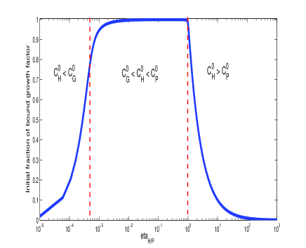
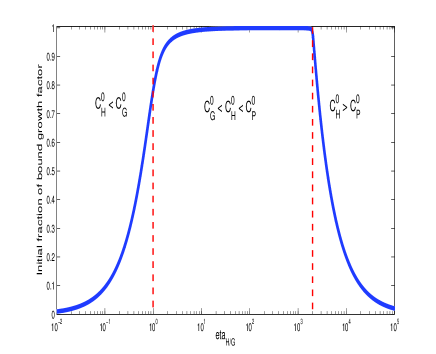
Figure 4: Theoretical curves for the equilibrium bound fraction of growth factor prior to release. The curves are calculated using the formulae (A.1). In the figure on the left, $\eta_{\mbox{\tiny H/P}}$ is varied and the remaining non-dimensional parameters are fixed. In the figure on the right, $\eta_{\mbox{\tiny H/G}}$ is varied with the other parameters fixed. The parameter values used are $D_{\mbox{\tiny G}}^{*}=6$, $D_{\mbox{\tiny H}}^{*}=3$, $\eta_{\mbox{\tiny H/G}}/\eta_{\mbox{\tiny H/P}}=2000$, $\theta=9\times 10^{-3}$, $K_{b{\mbox{\tiny P}}}=3000$ and $K_{\mbox{\tiny G-H}}^{\mbox{\tiny D}}=7.5\times 10^{-9}$M (Nugent & Edelman (1992)).

We have a ‘large’ growth factor flux for the first three cases in (3.3) because for each of these regimes, there is a substantial free component that can diffuse. For example, for the first case, $c_{\mbox{\tiny H}}^{\mbox{\tiny T}}<c_{\mbox{\tiny G}}^{\mbox{\tiny T}}$ and $c_{\mbox{\tiny H}}^{\mbox{\tiny T}}<c_{\mbox{\tiny P}}^{\mbox{\tiny 0}}$, we have $c_{\mbox{\tiny G}}\sim c_{\mbox{\tiny G}}^{\mbox{\tiny T}}-c_{\mbox{\tiny H}}^{\mbox{\tiny T}}$. For the boundary and initial conditions of (2.15), this free drug will clear the system to leading order on the time scale $t=O(L^{2}/D_{\mbox{\tiny GH}})$. However, once the free component has cleared, the remaining bound component in the bulk will be governed by the fourth regime of (3.3), and this will clear the system on the long time scale $t=O(L^{2}/(\varepsilon D_{\mbox{\tiny GH}}))\gg O(L^{2}/D_{\mbox{\tiny GH}})$. Similar remarks apply to the second and third regimes in (3.3). Hence, if the matrix is prepared with $K_{b{\mbox{\tiny H}}},K_{b{\mbox{\tiny P}}}\gg 1$, and if our governing model is appropriate, then we are assured that at least a fraction of the growth factor will release on the slow time scale $t=O(L^{2}/(\varepsilon D_{\mbox{\tiny GH}}))$. Furthermore, we predict that almost all of the growth factor will release slowly if the matrix is prepared with $c_{\mbox{\tiny H}}^{\mbox{\tiny 0}}/c_{\mbox{\tiny G}}^{\mbox{\tiny 0}}>1$ and $c_{\mbox{\tiny P}}^{\mbox{\tiny 0}}/c_{\mbox{\tiny H}}^{\mbox{\tiny 0}}>1$; notice that it is not required that these fractions be large; see Figure 4. However, we should caution that if there is a substantial component of free peptide (which is not included in the model described here), then there can still be a significant amount of free growth factor that can release on a fast diffusion time scale.

The two stage release behaviour just described has been observed in experiments (see Section 4), where one sometimes sees a proportion of the growth factor releasing quickly over a period of some days (which could correspond to free growth factor releasing on a diffusion time scale) followed by much slower release of the remaining fraction (which could correspond to a strongly retained bound component releasing on a longer time scale such as that described above).

Incorporating free peptide in the analysis

We now consider the case where a substantial fraction of the peptide remains free and competes with the covalently bound peptide for free heparin. We assume that heparin bound to free peptide has the same binding behaviour for growth factor as free heparin. The essence of our results above carry over, as we now explain. We suppose that the conditions (3.4) hold, and that the ratio of peptide covalently attached to the fibrin, $r$, has been quantified. Then the concentration of cross-linked peptide in the system is $rc_{\mbox{\tiny P}}^{\mbox{\tiny 0}}$, and since $c_{\mbox{\tiny P}}^{\mbox{\tiny 0}}>c_{\mbox{\tiny H}}^{\mbox{\tiny 0}}$, the initial concentration of heparin that is bound to cross-linked peptide is, to leading order, $rc_{\mbox{\tiny H}}^{\mbox{\tiny 0}}$. Since in turn $c_{\mbox{\tiny H}}^{\mbox{\tiny 0}}>c_{\mbox{\tiny G}}^{\mbox{\tiny 0}}$, the initial concentration of growth factor trapped by the delivery system is, to leading order, $rc_{\mbox{\tiny G}}^{\mbox{\tiny 0}}$. It follows that a fraction $(1-r)$ approximately of the growth factor will diffuse out of the system over a diffusion time scale. Hence, the final recommendation, which we add to (3.4), is that $c_{\mbox{\tiny G}}^{\mbox{\tiny 0}}$ should be chosen so that $rc_{\mbox{\tiny G}}^{\mbox{\tiny 0}}$ is sufficiently large for the therapy to be effective.

3.1.2 Numerical Solutions

Two different procedures were used to numerically integrate the initial boundary value problem (2.15). In one method, simple explicit time-stepping was used to update the values of $c_{\mbox{\tiny G}}^{\mbox{\tiny T}}$, $c_{\mbox{\tiny H}}^{\mbox{\tiny T}}$, with the other quantities being then updated using (A.1). Centred difference approximations were used for $c_{\mbox{\tiny G}xx}$, $c_{\mbox{\tiny H}xx}$, $c_{\mbox{\tiny GH}xx}$, and the no-flux conditions on $x=0$ were handled by introducing a fictitious line in the usual way. In the other method, the system was numerically integrated using the MAPLE command pdsolve/numeric, which is based on a centred implict finite difference scheme. Good agreement was obtained between the two schemes and with known analytical results.

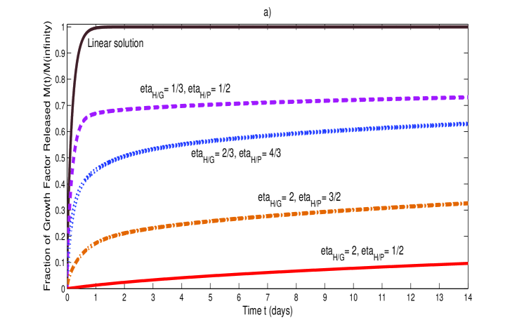
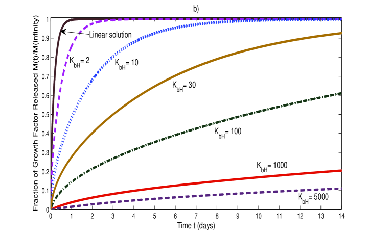
Figure 5: Numerical solutions of the initial boundary value problem (2.15). We display the predicted fraction of total growth factor released over a two week period. We use the parameter values $D_{\mbox{\tiny G}}^{*}=6$, $D_{\mbox{\tiny H}}^{*}=3$, $\theta=9\times 10^{-3}$, $K_{b{\mbox{\tiny P}}}=3000$ throughout. In (a), $K_{b{\mbox{\tiny H}}}=8000$ with various $\eta_{\mbox{\tiny H/G}}$, $\eta_{\mbox{\tiny H/P}}$ values indicated on the curves. In (b), $\eta_{\mbox{\tiny H/G}}=1000$, $\eta_{\mbox{\tiny H/P}}=1/40$ with various $K_{b{\mbox{\tiny H}}}$ values indicated on the curves.

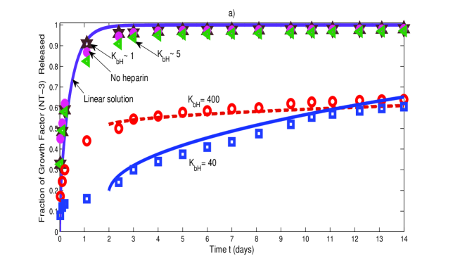
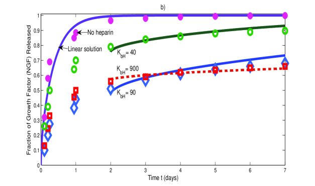
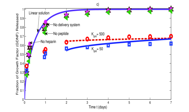
Figure 6: Comparison of experimental and theoretical release profiles. The curves are theoretical and the symbols are experimental. In the figure, (a) has data for NT-3 taken from Taylor et al. (2004), (b) has data for NGF taken from Wood et al. (2007), and (c) has data for GDNF taken from Wood et al. (2008). The values of $K_{b{\mbox{\tiny H}}}$ used to generate the theoretical curves are given on them and the remaining parameters used can be found in Table Appendix of the Appendix. In (a), two approximate $K_{b{\mbox{\tiny H}}}$ values for experimental data are also given.

In Figure 5, we display numerical profiles for the fraction of total growth factor that has released from the system as a function of time over a period of a fortnight. Four of the five release profiles displayed in Figure 5 (a) correspond to the case $K_{b{\mbox{\tiny H}}},K_{b{\mbox{\tiny P}}}\gg 1$, the regime we recommend for matrix preparation. The other parameter values are all $O(1)$, and can be found either on the figure or in its caption. The fifth profile, the top curve in the figure, corresponds to the case of no drug delivery system, and has been included for comparison. In this case, all of the growth factor is free in the gel, and its concentration is governed by the usual linear diffusion equation (see Section 3.2.1). The other four curves correspond to the four asymptotic regimes identified in the previous Section. We observe for these that the growth factor release rate becomes slow after a period of appproximately a day, and this is easily interpreted. The fast initial release phase corresponds to the rapid out-diffusion of free growth factor on a diffusion time scale; notice that this period coincides (tellingly) with the period over which the growth factor releases when there is no delivery system. Once the free component has substantially exited the system, the remaining bound fraction releases slowly over a long time scale, as previously explained. In all cases, the numerical results are consistent with the asymptotic predictions.

In Figure 5 (b), we display numerical solutions to (2.15) for $K_{b{\mbox{\tiny P}}},\eta_{\mbox{\tiny H/G}}\gg 1$, and for various values of $K_{b{\mbox{\tiny H}}}$. These parameters correspond to the heparin being strongly retained by the peptide, and the initial concentration of heparin greatly exceeding that of the growth factor. However, we see from the figure that this is not sufficient to guarantee slow release of growth factor. For values $K_{b{\mbox{\tiny H}}}=O(1)$, which correspond to moderate retention of growth factor, the growth factor will release over a period of some days. This compares unfavourably with the results displayed in Figure 5 (a) where both $K_{b{\mbox{\tiny P}}}$ and $K_{b{\mbox{\tiny H}}}$ are large and we have slow release in all cases even though the values for $\eta_{\mbox{\tiny H/G}}$ there are only $O(1)$.

3.2 Assessing the validity of the model experimentally

The appropriateness of the proposed governing mathematical model may be assessed experimentally for a particular system by simply omitting components from the polymerization mixture when preparing the fibrin gels. The governing mathematical model may then reduce considerably, making it easier to compare its predictions with experimental data and enabling parameter estimation. We suggest that such simpler systems should be assessed experimentally as a preliminary to consideration of the complete release system. We consider two such cases, and then make a brief remark concerning the full system.

3.2.1 No heparin

If in the preparation of the fibrin matrices, no heparin is added to the fibrinogen solution, then $c_{\mbox{\tiny H}}=c_{\mbox{\tiny GH}}=c_{\mbox{\tiny HP}}=c_{\mbox{\tiny GHP}}=0$. The dimensional form for the governing equations reduces to:

$$\frac{\partial c_{\mbox{\tiny G}}}{\partial t}=D_{\mbox{\tiny G}}\frac{\partial^{2}c_{\mbox{\tiny G}}}{\partial x^{2}},$$ (3.5)

$$\frac{\partial c_{\mbox{\tiny G}}}{\partial x}=0\mbox{ on }x=0,\hskip 5.69046ptc_{\mbox{\tiny G}}=0\mbox{ on }x=L,\hskip 5.69046ptc_{\mbox{\tiny G}}=c_{\mbox{\tiny G}}^{0}\mbox{ at }t=0,$$

and this is easily solved by separating variables (Crank (1975)) to obtain:

$$c_{\mbox{\tiny G}}(x,t)=\frac{{4c_{\mbox{\tiny G}}^{0}}}{\pi}\sum\limits_{n=1}^{\infty}\frac{{(-1)^{n+1}}}{{2n-1}}\exp\left({\frac{{-(2n-1)^{2}\pi^{2}D_{\mbox{\tiny G}}t}}{4L^{2}}}\right)\cos\left(\frac{{(2n-1)\pi x}}{2L}\right).$$

The total amount of growth factor released from the fibrin matrix by time $t$ is then given by:

$$M(t)=Lc_{\mbox{\tiny G}}^{0}-\int\limits_{0}^{L}c_{\mbox{\tiny G}}(x,t)dx,$$

from which it follows that the fraction of the available growth factor released by time $t$ is:

$$\frac{M(t)}{M(\infty)}={1-\frac{8}{{\pi^{2}}}\sum\limits_{n=1}^{\infty}\frac{1}{{(2n-1)^{2}}}\exp\left(\frac{{-(2n-1)^{2}\pi^{2}D_{\mbox{\tiny G}}t}}{4L^{2}}\right)}.$$ (3.6)

This expression contains only one unknown parameter, $D_{\mbox{\tiny G}}$, and it predicts that the growth factor should release on the time scale $t=O(L^{2}/D_{\mbox{\tiny G}})$, which for the matrices described here and typical growth factors corresponds to a period of some days. We suggest a four day release experiment and at least three data points per day for the fraction of growth factor released. This release data may then be compared with (3.6). If there is a poor match between the experimental and theoretical profiles, or if one finds that an unreasonable value for $D_{\mbox{\tiny G}}$ must be used to obtain an acceptable fit, then the appropriateness of the model for the delivery system of interest is called into question. It may be that some other process not incorporated in the modelling is significantly affecting the release behaviour.

3.2.2 No growth factor and peptide

If both growth factor and peptide are omitted from the polymerization mixture, then $c_{\mbox{\tiny G}}=c_{\mbox{\tiny P}}=c_{\mbox{\tiny GH}}=c_{\mbox{\tiny HP}}=c_{\mbox{\tiny GHP}}=0$. The only surviving species in the model is free heparin, and its concentration is governed by an initial boundary value problem identical in structure to (3.5); simply substitute $G$ with $H$ in (3.5) and (3.6). We now suggest a four day release experiment for the heparin with at least three data points per day for the fraction of heparin released. The experimental and theoretical release results may then be compared, providing a second test of the validity of the model. If the correspondence between theory and experiment is good, then the heparin diffusivity $D_{\mbox{\tiny H}}$ is estimated (of course the value obtained must be consistent with previous estimates; it must have the correct order of magnitude).

3.2.3 The full system

If the model passes the tests set for it in the previous two subsections, one may proceed to preparing the matrix with all components included. If the matrix is prepared in accordance with the recommendations (3.4), one should experimentally observe the growth factor release rate become slow after a period of a few days if the model is valid.

4 Comparison with experimental data

We now compare the theoretical release profiles generated by the model with in vitro experimental release data. For experimental data where there is no delivery system or no heparin, we make the comparison with the model for all times using the analytical expression (3.6). However, for experimental data where the full delivery system is present, we do not attempt to compare the model results with experimental data in the first two days of release since free peptide may play a significant role in this period, and the model does not track the concentration of this species. In fact, to incorporate the effect of free peptide would require the inclusion of three more species in the model: free peptide, free peptide-heparin complex, and free peptide-heparin-growth factor complex; see Wood et al. (2007). This would add three reaction-diffusion equations to the governing mathematical model, and would complicate the analysis considerably. However, after a period of some days, all of these species should have substantially diffused out of the system since there is no mechanism to replenish them (the covalently bound peptide does not dissociate), and the species that then remain do form part of the model described here. We should say that it is not difficult to fit the model results with complete release profiles that include the first few days, but this would require the selection of parameters in the model that are not compatible with the experimental conditions. The numerical solutions displayed in Figure 5 (a) do have the qualitative character of many experimental profiles.

In selecting parameter values for the model, we use wherever possible the values used in the experiments. We always use the same heparin to growth factor ratio $\eta_{\mbox{\tiny H/G}}$ and heparin to peptide ratio $\eta_{\mbox{\tiny H/P}}$ as used in the experiments. Where estimates for the diffusivities can be found, either in the experimental paper in question, or elsewhere, we use them. Where a value for $D_{\mbox{\tiny G}}$ is not available, we estimate it by fitting an experimental profile for no delivery system to the corresponding theoretical release profile (3.6). For $D_{\mbox{\tiny GH}}$, we then select a value which has order of magnitude 10^-5 cm²/min, and which is such that $D_{\mbox{\tiny GH}}<D_{\mbox{\tiny G}},D_{\mbox{\tiny H}}$. The values for $K_{b{\mbox{\tiny P}}}=c_{\mbox{\tiny P}}^{\mbox{\tiny 0}}/K_{\mbox{\tiny H-P}}^{\mbox{\tiny D}}$ are calculated using the given values for $c_{\mbox{\tiny P}}^{\mbox{\tiny 0}}$ and $K_{\mbox{\tiny H-P}}^{\mbox{\tiny D}}=8.67\times 10^{-8}$ M. This is probably an over-estimate since we are beginning our simulation after day two and unbound peptide will have been lost, reducing the value for $c_{\mbox{\tiny P}}^{\mbox{\tiny 0}}$. A similar remark applies to the values of $c_{\mbox{\tiny G}}^{\mbox{\tiny 0}}$ and $c_{\mbox{\tiny H}}^{\mbox{\tiny 0}}$. However, the values for $K_{b{\mbox{\tiny P}}}$ are of the order of thousands, and adjusting them by a factor of two or so will have very little effect on the resulting profiles. The selection of appropriate values for $K_{b{\mbox{\tiny H}}}=c_{\mbox{\tiny H}}^{\mbox{\tiny 0}}/K_{\mbox{\tiny G-H}}^{\mbox{\tiny D}}$ is a much more delicate issue though because its values range considerably in the experiments and the behaviour is usually strongly dependent on this value. Unfortunately, both numbers involved in the calculation of $K_{b{\mbox{\tiny H}}}$ are uncertain here since $c_{\mbox{\tiny H}}^{\mbox{\tiny 0}}$ needs to be reduced as explained above and only order of magnitude estimates are available for $K_{\mbox{\tiny G-H}}^{\mbox{\tiny D}}$. Hence, we use $K_{b{\mbox{\tiny H}}}$ as a fitting parameter, but insist that it has the same order of magnitude as $c_{\mbox{\tiny H}}^{\mbox{\tiny 0}}/K_{\mbox{\tiny G-H}}^{\mbox{\tiny D}}$ where $c_{\mbox{\tiny H}}^{\mbox{\tiny 0}}$ is the value given in the experiment and $K_{\mbox{\tiny G-H}}^{\mbox{\tiny D}}$ is the order of magnitude estimate for this dissociation constant.

We have chosen to compare the model results with experimental data drawn from three studies: (a) Taylor et al. (2004), (b) Wood et al. (2007), and (c) Wood et al. (2008); we shall subsequently refer to these as (a),(b),(c), and this labelling has also been used in Figure 6 where the comparison between the model and the experimental data is given. In (a), (b), (c) the growth factors used are NT-3, NGF and GDNF, respectively. In Figure 6, we also display in each case the solution (3.6) with the appropriate value for $D_{\mbox{\tiny G}}$, which is the theoretical prediction when there is no delivery system or no heparin. In Figure 6 (a), we display experimental data with $K_{b{\mbox{\tiny H}}}\sim 1$ and $K_{b{\mbox{\tiny H}}}\sim 5$, but we do not attempt to fit this data other than to comment that it follows quite closely the behaviour of the solution (3.6).

We note that the correspondence between the model and experimental data is satisfactory in all cases. It is clear that for $K_{b{\mbox{\tiny H}}}\gg 1$, the experimental release rates becomes slow after a few days, which is consistent with the theoretical prediction. For $O(1)$ values of $K_{b{\mbox{\tiny H}}}$ (Figure 6 (a)), the experimental realease rates are comparable to that for no delivery system. The experimental release profiles for data corresponding to no delivery system or no heparin are adequately described by (3.6).

5 Discussion

We summarise our results.

• We have shown that for conditions of typical interest, the governing mathematical model may be reduced to a system of just two partial differential equations, and that the release behaviour is frequently dominated by the values of two non-dimensional parameters. If the model is valid for a particular system, there will usually be slow passive release of at least a fraction of the growth factor if the fibrin matrices are prepared with the concentration of crosslinked peptide greatly exceeding the dissociation constant of heparin from peptide, and the concentration of heparin greatly exceeding the dissociation constant of growth factor from heparin. It is noteworthy that these criteria do not preclude slow release for growth factors that bind heparin with low affinity. We also note the value of having reliable estimates for the two dissociation constants in the system.

• It is experimentally convenient to vary the ratios of heparin to growth factor and of heparin to peptide in the polymerisation mixture for the gels to determine optimal conditions for slow passive release. However, these ratios are not usually the key parameters, and where this strategy does result in slow release, we have found that it is because the binding constants have strayed into the regime referred to in the point immediately above. Our results indicate that the ratios of heparin to growth factor and of heparin to peptide in the polymerisation mixture need neither be large nor small for slow release.

• For the first time, theoretical release profiles generated by the model are compared directly with in vitro experimental data. It is found that once the free components have cleared the system, the correspondence between experimental and theoretical results is satisfactory. In particular, our predictions concerning conditions that will give rise to slow passive release are confirmed.

• It may be possible to partially unpick the system experimentally by simply omitting components in the polymerization mixture for the fibrin gels. For example, if heparin is omitted from the polymerization mixture, the governing mathematical model reduces to a standard linear diffusion equation for the growth factor, and theoretical predictions may then be readily compared with experimental data to help validate the model and estimate a diffusivity; see Section 3.2.

Acknowledgement

VTNT thanks the Mathematics Applications Consortium for Science and Industry (MACSI) and Science Foundation Ireland (SFI) for their financial support (06/MI/005). MGM thanks MACSI for its support and NUI Galway for the award of a travel grant.

Appendix

Species concentrations in terms of total growth factor and total heparin

Solving the six algebraic expressions (2.10)₆, (2.13)₁, (2.14) for the concentrations of the six species $c_{\mbox{\tiny G}}$, $c_{\mbox{\tiny H}}$, $c_{\mbox{\tiny GH}}$, $c_{\mbox{\tiny P}}$, $c_{\mbox{\tiny HP}}$, $c_{\mbox{\tiny GHP}}$ in terms of the total concentration of growth factor, $c_{\mbox{\tiny G}}^{\mbox{\tiny T}}$, and heparin, $c_{\mbox{\tiny H}}^{\mbox{\tiny T}}$, gives:

$$c_{\mbox{\tiny G}}(c_{\mbox{\tiny G}}^{\mbox{\tiny T}},c_{\mbox{\tiny H}}^{\mbox{\tiny T}})=\frac{c_{\mbox{\tiny G}}^{\mbox{\tiny T}}-\eta_{\mbox{\tiny H/G}}c_{\mbox{\tiny H}}^{\mbox{\tiny T}}-\frac{\eta_{\mbox{\tiny H/G}}}{K_{b{\mbox{\tiny H}}}}+\sqrt{\left(c_{\mbox{\tiny G}}^{\mbox{\tiny T}}-\eta_{\mbox{\tiny H/G}}c_{\mbox{\tiny H}}^{\mbox{\tiny T}}-\frac{\eta_{\mbox{\tiny H/G}}}{K_{b{\mbox{\tiny H}}}}\right)^{2}+\frac{4\eta_{\mbox{\tiny H/G}}c_{\mbox{\tiny G}}^{\mbox{\tiny T}}}{K_{b{\mbox{\tiny H}}}}}}{2},$$

$$c_{\mbox{\tiny P}}(c_{\mbox{\tiny H}}^{\mbox{\tiny T}})=\frac{1-\frac{1}{K_{b{\mbox{\tiny P}}}}-\eta_{\mbox{\tiny H/P}}c_{\mbox{\tiny H}}^{\mbox{\tiny T}}+\sqrt{\left(\eta_{\mbox{\tiny H/P}}c_{\mbox{\tiny H}}^{\mbox{\tiny T}}-1-\frac{1}{K_{b{\mbox{\tiny P}}}}\right)^{2}+\frac{4\eta_{\mbox{\tiny H/P}}c_{\mbox{\tiny H}}^{\mbox{\tiny T}}}{K_{b{\mbox{\tiny P}}}}}}{2},$$

$$c_{\mbox{\tiny GH}}(c_{\mbox{\tiny G}}^{\mbox{\tiny T}},c_{\mbox{\tiny H}}^{\mbox{\tiny T}})=\frac{\frac{\eta_{\mbox{\tiny H/G}}}{\eta_{\mbox{\tiny H/P}}}(1-c_{\mbox{\tiny P}}(c_{\mbox{\tiny H}}^{\mbox{\tiny T}}))\left\{\frac{1}{K_{b{\mbox{\tiny P}}}c_{\mbox{\tiny P}}(c_{\mbox{\tiny H}}^{\mbox{\tiny T}})}+\frac{1}{1+\frac{K_{b{\mbox{\tiny H}}}\theta c_{\mbox{\tiny G}}(c_{\mbox{\tiny G}}^{\mbox{\tiny T}},c_{\mbox{\tiny H}}^{\mbox{\tiny T}})}{\eta_{\mbox{\tiny H/G}}(1+\theta)}}\right\}-\frac{\eta_{\mbox{\tiny H/G}}(c_{\mbox{\tiny G}}^{\mbox{\tiny T}}-c_{\mbox{\tiny G}}(c_{\mbox{\tiny G}}^{\mbox{\tiny T}},c_{\mbox{\tiny H}}^{\mbox{\tiny T}}))}{K_{b{\mbox{\tiny H}}}c_{\mbox{\tiny G}}(c_{\mbox{\tiny G}}^{\mbox{\tiny T}},c_{\mbox{\tiny H}}^{\mbox{\tiny T}}))}}{1+\frac{\frac{K_{b{\mbox{\tiny P}}}c_{\mbox{\tiny P}}(c_{\mbox{\tiny H}}^{\mbox{\tiny T}})}{1+\theta}}{1+\frac{K_{b{\mbox{\tiny H}}}\theta c_{\mbox{\tiny G}}(c_{\mbox{\tiny G}}^{\mbox{\tiny T}},c_{\mbox{\tiny H}}^{\mbox{\tiny T}})}{\eta_{\mbox{\tiny H/G}}(1+\theta)}}},$$

(A.1)

$$c_{\mbox{\tiny GHP}}(c_{\mbox{\tiny G}}^{\mbox{\tiny T}},c_{\mbox{\tiny H}}^{\mbox{\tiny T}})=c_{\mbox{\tiny G}}^{\mbox{\tiny T}}-c_{\mbox{\tiny G}}(c_{\mbox{\tiny G}}^{\mbox{\tiny T}},c_{\mbox{\tiny H}}^{\mbox{\tiny T}})-c_{\mbox{\tiny GH}}(c_{\mbox{\tiny G}}^{\mbox{\tiny T}},c_{\mbox{\tiny H}}^{\mbox{\tiny T}}),$$

$$c_{\mbox{\tiny HP}}(c_{\mbox{\tiny G}}^{\mbox{\tiny T}},c_{\mbox{\tiny H}}^{\mbox{\tiny T}})=\frac{\frac{1}{\eta_{\mbox{\tiny H/P}}}(1-c_{\mbox{\tiny P}}(c_{\mbox{\tiny H}}^{\mbox{\tiny T}}))-\frac{K_{b{\mbox{\tiny P}}}c_{\mbox{\tiny GH}}(c_{\mbox{\tiny G}}^{\mbox{\tiny T}},c_{\mbox{\tiny H}}^{\mbox{\tiny T}})c_{\mbox{\tiny P}}(c_{\mbox{\tiny H}}^{\mbox{\tiny T}})}{\eta_{\mbox{\tiny H/G}}(1+\theta)}}{1+\frac{K_{b{\mbox{\tiny H}}}c_{\mbox{\tiny G}}(c_{\mbox{\tiny G}}^{\mbox{\tiny T}},c_{\mbox{\tiny H}}^{\mbox{\tiny T}})\theta}{\eta_{\mbox{\tiny H/G}}(1+\theta)}},$$

$$c_{\mbox{\tiny H}}(c_{\mbox{\tiny G}}^{\mbox{\tiny T}},c_{\mbox{\tiny H}}^{\mbox{\tiny T}})=c_{\mbox{\tiny H}}^{\mbox{\tiny T}}-c_{\mbox{\tiny HP}}(c_{\mbox{\tiny G}}^{\mbox{\tiny T}},c_{\mbox{\tiny H}}^{\mbox{\tiny T}})-(c_{\mbox{\tiny GH}}(c_{\mbox{\tiny G}}^{\mbox{\tiny T}},c_{\mbox{\tiny H}}^{\mbox{\tiny T}})+c_{\mbox{\tiny GHP}}(c_{\mbox{\tiny G}}^{\mbox{\tiny T}},c_{\mbox{\tiny H}}^{\mbox{\tiny T}}))/\eta_{\mbox{\tiny H/G}}.$$

Hence, in the model considered here, it is sufficient to solve for $c_{\mbox{\tiny G}}^{\mbox{\tiny T}}$ and $c_{\mbox{\tiny H}}^{\mbox{\tiny T}}$.

The data used to generate the theoretical curves in Figure 6. Unmarked data is taken from the paper referred to in its column. The markings on the remaining data are explained below the table. Figure 6 (a) Figure 6 (b) Figure 6 (c) Symbol NT-3 (Taylor et al. (2004)) NGF (Wood et al. (2007)) GDNF (Wood et al. (2008)) Units $D_{\mbox{\tiny G}}$ & ${2.5\times 10^{-5}}^{(a)}$ $9.7\times 10^{-5}$ ${2.0\times 10^{-5}}^{(a)}$ cm²/min $D_{\mbox{\tiny H}}$ ${3.0\times 10^{-5}}^{(b)}$ $9.1\times 10^{-5}$ ${3.0\times 10^{-5}}^{(b)}$ cm²/min $D_{\mbox{\tiny GH}}$ ${1.0\times 10^{-5}}^{(c)}$ $7.5\times 10^{-5}$ ${1.5\times 10^{-5}}^{(a)}$ cm²/min $K_{\mbox{\tiny G-H}}^{\mbox{\tiny D}}$ ${1.5\times 10^{-7}}^{(a)}$ ${0.33\times 10^{-7}}^{(a)}$ ${1.25\times 10^{-7}}^{(a)}$ M $K_{\mbox{\tiny H-P}}^{\mbox{\tiny D}}$ ${8.67\times 10^{-8}}^{(d)}$ ${8.67\times 10^{-8}}^{(d)}$ ${8.67\times 10^{-8}}^{(d)}$ M $c_{\mbox{\tiny P}}^{\mbox{\tiny 0}}$ $2.3\times 10^{-4}$ $2.5\times 10^{-4}$ $2.5\times 10^{-4}$ M $c_{\mbox{\tiny G}}^{\mbox{\tiny 0}}$ $7.4\times 10^{-9}$ $7.4\times 10^{-9}$ $3.1\times 10^{-9}$ M ^(a) Estimated from data in Taylor et al. (2004); Wood et al. (2007, 2008). ^(b) Gaigalas et al. (1995). ^(c) Saltzman et al. (1994). ^(d) ${\mbox{\tiny K}}_{\mbox{\tiny R}}=78$ min^-1 (Olson et al. (1981)) and ${\mbox{\tiny K}}_{\mbox{\tiny F}}=9.0\times 10^{8}$ M^-1min^-1 (Tyler-Cross et al. (1994, 1996); Kridel et al. (1996)).

References

• (1)
• (2)
• Alberts et al. (2002) Alberts, B., Johnson, A., Lewis, J., Raff, M., Roberts, K. & Walter, P. (2002) Molecular Biology of the Cell, 4th edition. New York: Garland Science.
• Crank (1975) J. Crank (1975) The Mathematics of Diffusion. Oxford: Oxford University Press.
• Gaigalas et al. (1995) Gaigalas, A.K., Hubbard, J.B., Lesage, R. & Atha, D.H. (1995) Physical characterization of heparin by light scattering, Journal of Pharmaceutical Sciences, 84, 355–359.
• Kridel et al. (1996) Kridel, S.J., Chan, W.W. & Knauer, D.J. (1996) Requirement of lysine residues outside of the proposed pentasaccharide binding region for high affinity heparin binding and activation of human antithrombin III, Journal of Biological Chemistry, 271, 20935–20941.
• Lin & Metters (2006) Lin, C.C. & Metters, A.T. (2006) Hydrogels in controlled release formulations: Network design and mathematical modeling, Advanced Drug Delivery Reviews, 58, 1379–1408.
• Maxwell et al. (2005) Maxwell, D.J., Hicks, B.C., Parsons, S. & Sakiyama-Elbert, S.E. (2005) Development of rationally designed affinity-based drug delivery systems, Acta Biomaterialia, 1, 101–113.
• Nugent & Edelman (1992) Nugent, M.A. & Edelman, E.R. (1992) Kinetics of basic fibroblast growth factor binding to its receptor and heparan sulfate proteoglycan: a mechanism for cooperativity, Journal of Biological Chemistry, 31, 8876–8883.
• Olson et al. (1981) Olson, S.T., Srinivasan, K.R., Bj$\ddot{o}$rk, I. & Shore, J.D. (1981) Binding of high affinity heparin to antithrombin III. Stopped flow kinetic studies of the binding interaction, Biochemistry, 256, 11073–11079.
• Sakiyama et al. (1999) Sakiyama, S.E., Schense, J.C. & Hubbell, J.A. (1999) Incorporation of heparin-binding peptides into fibrin gels enhances neurite extension: an example of designer matrices in tissue engineering, FASEB J., 13, 2214–2224.