Sparse principal component analysis and iterative thresholding

Abstract

Principal component analysis (PCA) is a classical dimension reduction method which projects data onto the principal subspace spanned by the leading eigenvectors of the covariance matrix. However, it behaves poorly when the number of features $p$ is comparable to, or even much larger than, the sample size $n$. In this paper, we propose a new iterative thresholding approach for estimating principal subspaces in the setting where the leading eigenvectors are sparse. Under a spiked covariance model, we find that the new approach recovers the principal subspace and leading eigenvectors consistently, and even optimally, in a range of high-dimensional sparse settings. Simulated examples also demonstrate its competitive performance.

1 Introduction

In many contemporary datasets, if we organize the $p$-dimensional observations $x_{1},\ldots,x_{n}$, into the rows of an $n\times p$ data matrix $X$, the number of features $p$ is often comparable to, or even much larger than, the sample size $n$. For example, in biomedical studies, we usually have measurements on the expression levels of tens of thousands of genes, but only for tens or hundreds of individuals. One of the crucial issues in the analysis of such “large $p$” datasets is dimension reduction of the feature space.

As a classical method, principal component analysis (PCA) pear01 , hote33 reduces dimensionality by projecting the data onto the principal subspace spanned by the $m$ leading eigenvectors of the population covariance matrix $\Sigma$, which represent the principal modes of variation. In principle, one expects that for some $m<p$, most of the variance in the data is captured by these $m$ modes. Thus, PCA reduces the dimensionality of the feature space while retaining most of the information in data. In addition, projection to a low-dimensional space enables visualization of the data. In practice, $\Sigma$ is unknown. Classical PCA then estimates the leading population eigenvectors by those of the sample covariance matrix $S$. It performs well in the traditional data setting where $p$ is small and $n$ is large ande63 .

In high-dimensional settings, a collection of data can be modeled by a low-rank signal plus noise structure, and PCA can be used to recover the low-rank signal. In particular, each observation vector $x_{i}$ can be viewed as an independent instantiation of the following generative model:

$$x_{i}=\mu+Au_{i}+\sigma z_{i}.$$ (1)

Here, $\mu$ is the mean vector, $A$ is a $p\times\bar{m}$ deterministic matrix of factor loadings, $u_{i}$ is an $\bar{m}$-vector of random factors, $\sigma>0$ is the noise level and $z_{i}$ is a $p$-vector of white noise. For instance, in chemometrics, $x_{i}$ can be a vector of the logarithm of the absorbance or reflectance spectra measured with noise, where the columns of $A$ are characteristic spectral responses of different chemical components, and $u_{i}$’s the concentration levels of these components vafi09 . The number of observations are relatively few compared with the number of frequencies at which the spectra are measured. In econometrics, $x_{i}$ can be the returns for a collection of assets, where the $u_{i}$’s are the unobservable random factors tsay05 . The assumption of additive white noise is reasonable for asset returns with low frequencies (e.g., monthly returns of stocks). Here, people usually look at tens or hundreds of assets simultaneously, while the number of observations are also at the scale of tens or hundreds. In addition, model (1) represents a big class of signal processing problems wk85 . Without loss of generality, we assume $\mu=0$ from now on.

In this paper, our primary interest lies in PCA of high-dimensional data generated as in (1). Let the covariance matrix of $u_{i}$ be $\Phi$ which is of full rank. Suppose that $A$ has full column rank and that $u_{i}$ and $z_{i}$ are independent. Then the covariance matrix of $x_{i}$ becomes

$$\Sigma=A\Phi A^{\prime}+\sigma^{2}I=\sum_{j=1}^{\bar{m}}\lambda_{j}^{2}q_{j}q_{j}^{\prime}+\sigma^{2}I.$$ (2)

Here, $\lambda_{1}^{2}\geq\cdots\geq\lambda_{\bar{m}}^{2}>0$ are the eigenvalues of $A\Phi A^{\prime}$, with $q_{j}$, $j=1,\ldots,\bar{m}$, the associated eigenvectors. Therefore, the $j$th eigenvalue of $\Sigma$ is $\lambda_{j}^{2}+\sigma^{2}$ for $j=1,\ldots,\bar{m}$, and $\sigma^{2}$ otherwise. Since there are $\bar{m}$ spikes $(\lambda_{1}^{2},\ldots,\lambda_{\bar{m}}^{2})$ in the spectrum of $\Sigma$, (2) has been called the spiked covariance model in the literature john01 . Note that we use $\lambda_{j}^{2}$ to denote the spikes rather than $\lambda_{j}$ used previously in the literature pajo07 . For data with such a covariance structure, it makes sense to project the data onto the low-dimensional subspaces spanned by the first few $q_{j}$’s. Here and after, $\bar{m}$ denotes the number of spikes in the model, and $m$ is the target dimension of the principal subspace to be estimated, which is no greater than $\bar{m}$.

Classical PCA encounters both practical and theoretical difficulties in high dimensions. On the practical side, the eigenvectors found by classical PCA involve all the $p$ features, which makes their interpretation challenging. On the theoretical side, the sample eigenvectors are no longer always consistent estimators. Sometimes, they can even be nearly orthogonal to the target direction. When both $n,p\to\infty$ with $n/p\to c\in(0,\infty)$, at different levels of rigor and generality, this phenomenon has been examined by a number of authors reva96 , lu02 , hora04 , paul07 , nadl08 , onat09 under model (2). See juma09 for similar results when $p\to\infty$ and $n$ is fixed.

In recent years, to facilitate interpretation, researchers have started to develop sparse PCA methodologies, where they seek a set of sparse vectors spanning the low-dimensional subspace that explains most of the variance. See, for example, jotrud03 , zohati06 , dagh07 , shhu08 , solo08 , witiha09 . These approaches typically start with a certain optimization formulation of PCA and then induce a sparse solution by introducing appropriate penalties or constraints.

On the other hand, when $\Sigma$ indeed has sparse leading eigenvectors in the current basis (perhaps after transforming the data), it becomes possible to estimate them consistently under high-dimensional settings via new estimation schemes. For example, under normality assumption, when $\Sigma$ only has a single spike, that is, when $\bar{m}=1$ in (2), Johnstone and Lu jolu09 proved consistency of PCA obtained on a subset of features with large sample variances when the leading eigenvalue is fixed and $(\log{p})/n\to 0$. Under the same single spike model, if in addition the leading eigenvector has exactly $k$ nonzero loadings, Amini and Wainwright amwa09 studied conditions for recovering the nonzero locations using the methods in jolu09 and dagh07 , and Shen et al. shshma11 established conditions for consistency of a sparse PCA method in shhu08 when $p\to\infty$ and $n$ is fixed. For the more general multiple component case, Paul and Johnstone pajo07 proposed an augmented sparse PCA method for estimating each of the leading eigenvectors, and showed that their procedure attains near optimal rate of convergence under a range of high-dimensional sparse settings when the leading eigenvalues are comparable and well separated. Notably, these methods all focus on estimating individual eigenvectors.

In this paper, we focus primarily on finding principal subspaces of $\Sigma$ spanned by sparse leading eigenvectors, as opposed to finding each sparse vector individually. One of the reasons is that individual eigenvectors are not identifiable when some leading eigenvalues are identical or close to each other. Moreover, if we view PCA as a dimension reduction technique, it is the low-dimensional subspace onto which we project data that is of the greatest interest.

We propose a new iterative thresholding algorithm to estimate principal subspaces, which is motivated by the orthogonal iteration method in matrix computation. In addition to the usual orthogonal iteration steps, an additional thresholding step is added to seek sparse basis vectors for the subspace. When $\Sigma$ follows the spiked covariance model and the sparsity of the leading eigenvectors are characterized by the weak-$\ell_{r}$ condition (10), the algorithm leads to a consistent subspace estimator adaptively over a wide range of high-dimensional sparse settings, and the rates of convergence are derived under an appropriate loss function (3). Moreover, for any individual leading eigenvector whose eigenvalue is well separated from the rest of the spectrum, our algorithm also yields an eigenvector estimator which adaptively attains optimal rate of convergence derived in pajo07 up to a multiplicative log factor. In addition, it has appealing model selection property in the sense that the resulting estimator only involves coordinates with large signal-to-noise ratios.

The contribution of the current paper is threefold. First, we propose to estimate principal subspaces. This is natural for the purpose of dimension reduction and visualization, and avoids the identifiability issue for individual eigenvectors. Second, we construct a new algorithm to estimate the subspaces, which is efficient in computation and easy to implement. Last but not least, we derive convergence rates of the resulting estimator under the spiked covariance model when the eigenvectors are sparse.

The rest of the paper is organized as follows. In Section 2, we frame the principal subspace estimation problem and propose the iterative thresholding algorithm. The statistical properties and computational complexity of the algorithm are examined in Sections 3 and 4 under normality assumption. Simulation results in Section 5 demonstrate its competitive performance. Section 6 presents the proof of the main theorems.

Reproducible code: The Matlab package SPCALab implementing the proposed method and producing the tables and figures of the current paper is available at the author’s website.

2 Methodology

2.1 Notation

We say $x$ is a $p$-vector if $x\in\mathbb{R}^{p}$, and we use $\|x\|_{2}$ to denote its Euclidean norm. For an $m\times n$ matrix $A$, its submatrix with rows indexed by $I$ and columns indexed by $J$ is denoted by $A_{IJ}$. If $I$ or $J$ includes all the indices, we replace it with a dot. For example, $A_{I\cdot}$ is the submatrix of $A$ with rows in $I$ and all columns. The spectral norm of $A$ is $\|A\|=\max_{\|x\|_{2}=1}\|Ax\|_{2}$, and the range, that is, the column subspace, of $A$ is $\operatorname{ran}(A)$. If $m\geq n$, and the columns of $A$ form an orthonormal set in $\mathbb{R}^{m}$, we say $A$ is orthonormal.

We use $C,C_{0},C_{1}$, etc. to represent constants, though their values might differ at different occurrences. For real numbers $a$ and $b$, let $a\vee b=\max(a,b)$ and $a\wedge b=\min(a,b)$. We write $a_{n}=O(b_{n})$, if there is a constant $C$, such that $|a_{n}|\leq Cb_{n}$ for all $n$, and $a_{n}=o(b_{n})$ if $a_{n}/b_{n}\to 0$ as $n\to\infty$. Moreover, we write $a_{n}\asymp b_{n}$ if $a_{n}=O(b_{n})$ and $b_{n}=O(a_{n})$. Throughout the paper, we use $\nu$ as the generic index for features, $i$ for observations, $j$ for eigenvalues and eigenvectors and $k$ for iterations in the algorithm to be proposed.

2.2 Framing the problem: Principal subspace estimation

When the covariance matrix $\Sigma$ follows model (2), its $j$th largest eigenvalue $\ell_{j}(\Sigma)=\lambda_{j}^{2}+\sigma^{2}$ for $j=1,\ldots,\bar{m}$ and equals $\sigma^{2}$ for all $j>\bar{m}$. Let $\operatorname{span}\{\cdot\}$ denote the linear subspace spanned by the vectors in the curly brackets. If for some $m\leq\bar{m}$, $\ell_{m}(\Sigma)>\ell_{m+1}(\Sigma)$, the principal subspace

$$\mathcal{P}_{m}=\operatorname{span}\{q_{1},\ldots,q_{m}\}$$

is defined, regardless of the behavior of the other $\ell_{j}(\Sigma)$’s. Therefore, it is an identifiable object for the purpose of estimation. Note that $\mathcal{P}_{\bar{m}}$ is always identifiable, because $\ell_{\bar{m}}(\Sigma)>\ell_{\bar{m}+1}(\Sigma)$. The primary goal of this paper is to estimate the principal subspace $\mathcal{P}_{m}$, for some $m\leq\bar{m}$ with $\ell_{m}(\Sigma)>\ell_{m+1}(\Sigma)$. More precisely, we require the gap $\ell_{m}(\Sigma)-\ell_{m+1}(\Sigma)=\lambda_{m}^{2}-\lambda_{m+1}^{2}\asymp\lambda_{1}^{2}$. Note that such an $m$ always exists, for example, the largest $m\leq\bar{m}$ such that $\lambda_{m}^{2}\asymp\lambda_{1}^{2}$. We allow the case of $m<\bar{m}$ partly because under certain circumstances, one might not be interested in $\mathcal{P}_{\bar{m}}$ directly. For example, to visualize the data, one might want to estimate $\mathcal{P}_{2}$ or $\mathcal{P}_{3}$ while $\bar{m}$ could be larger than $3$. In addition, sometimes $\mathcal{P}_{\bar{m}}$ might not be consistently estimable while some smaller principal subspace $\mathcal{P}_{m}$ is. In most part of the paper, we assume that an appropriate $m$ is given for convenience. In Section 3.5, we discuss how to choose $m$ and how to estimate $\bar{m}$ under normality assumption.

To measure the accuracy of an estimator $\widehat{\mathcal{S}}$ for a subspace $\mathcal{S}$, note that each linear subspace is associated with a unique projection matrix onto it. Let $P$ and $\widehat{P}$ be the projection matrices associated with $\mathcal{S}$ and $\widehat{\mathcal{S}}$, respectively. The distance between $\mathcal{S}$ and $\widehat{\mathcal{S}}$ is given by the spectral norm of the difference between $P$ and $\widehat{P}$: $\operatorname{dist}(\mathcal{S},\widehat{\mathcal{S}})=\|P-\widehat{P}\|$; see gova96 , Section 2.6.3. Thus, we can define a loss function by the squared distances between $\mathcal{S}$ and $\widehat{\mathcal{S}}$,

$$L(\mathcal{S},\widehat{\mathcal{S}})=\operatorname{dist}^{2}(\mathcal{S},\widehat{\mathcal{S}})=\|P-\widehat{P}\|^{2}.$$ (3)

By definition, this loss function measures the maximum possible discrepancy between the projections of any unit vector onto the two subspaces. The loss ranges in $[0,1]$, and equals zero if and only if $\widehat{\mathcal{S}}=\mathcal{S}$. When $\operatorname{dim}(\widehat{\mathcal{S}})\neq\operatorname{dim}(\mathcal{S})$, we have $L(\mathcal{S},\widehat{\mathcal{S}})=1$. Geometrically, it equals the squared sine of the largest canonical angle between $\mathcal{S}$ and $\widehat{\mathcal{S}}$ (stsu90 , Theorem 5.5). Throughout the paper, we use the loss function (3) for principal subspace estimation.

2.3 Orthogonal iteration

Given a positive definite matrix $A$, a standard technique to compute its leading eigenspace is orthogonal iteration gova96 . When only the first eigenvector is sought, it is also known as the power method.

To state the orthogonal iteration method, we note that for any $p\times m$ matrix $T$, when $p\geq m$, we could decompose it into the product of two matrices $T=QR$, where $Q$ is $p\times m$ orthonormal and $R$ is $m\times m$ upper triangular. This decomposition is called QR factorization and can be computed using Gram–Schmidt orthogonalization and other numerical methods gova96 . Suppose $A$ is $p\times p$, and we want to compute its leading eigenspace of dimension $m$. Starting with a $p\times m$ orthonormal matrix $Q^{(0)}$, orthogonal iteration generates a sequence of $p\times m$ orthonormal matrices $Q^{(k)}$, $k=1,2,\ldots\,$, by alternating the following two steps till convergence: [(2)]

Multiplication: $T^{(k)}=AQ^{(k-1)}$;

QR factorization: $Q^{(k)}R^{(k)}=T^{(k)}$. Denote the orthonormal matrix at convergence by $Q^{(\infty)}$. Then its columns are the leading eigenvectors of $A$, and $\operatorname{ran}(Q^{(\infty)})$ gives the eigenspace. In practice, one terminates the iteration once $\operatorname{ran}(Q^{(k)})$ stabilizes.

When we apply orthogonal iteration directly to the sample covariance matrix $S$, it gives the classical PCA result, which could be problematic in high dimensions. Observe that all the $p$ features are included in orthogonal iteration. When the dimensionality is high, not only the interpretation is hard, but the variance accumulated across all the features becomes so high that it makes consistent estimation impossible.

If the eigenvectors spanning $\mathcal{P}_{m}$ are sparse in the current basis, one sensible way to reduce estimation error is to focus only on those features at which the leading eigenvectors have large values, and to estimate other features by zeros. Of course, one introduces bias this way, but hopefully it is much smaller compared to the amount of variance thus reduced.

The above heuristics lead to the estimation scheme in the next subsection which incorporates this feature screening idea in orthogonal iteration.

2.4 Iterative thresholding algorithm

Let $S=\frac{1}{n}\sum_{i=1}^{n}x_{i}x_{i}^{\prime}$ be the sample covariance matrix. An effective way to incorporate feature screening into orthogonal iteration is to “kill” small coordinates of the $T^{(k)}$ matrix after each multiplication step, which leads to the estimation scheme summarized in Algorithm 1. Although the later theoretical study is conducted under normality assumption, Algorithm 1 itself is not confined to normal data.

Input:

1. [(4)]

2. Sample covariance matrix ${S}$;

3. Target subspace dimension $m$;

4. Thresholding function $\eta$, and threshold levels $\gamma_{nj}$, $j=1,\ldots,m$;

5. Initial orthonormal matrix $\widehat{Q}{}^{(0)}$.

Output: Subspace estimator $\widehat{\mathcal{P}}_{m}=\operatorname{ran}(\widehat{Q}{}^{(\infty)})$, where $\widehat{Q}{}^{(\infty)}$ denotes the $\widehat{Q}{}^{(k)}$ matrix at convergence.

repeat  Multiplication: $T^{(k)}=(t^{(k)}_{\nu j})={S}\widehat{Q}{}^{(k-1)}$; AlgoLine0.1

Thresholding: $\widehat{T}{}^{(k)}=(\widehat{t}{}^{(k)}_{\nu j})$, with $\widehat{t}{}^{(k)}_{\nu j}=\eta(t^{(k)}_{\nu j},\gamma_{nj})$; AlgoLine0.2

QR factorization: $\widehat{Q}{}^{(k)}\widehat{R}{}^{(k)}=\widehat{T}{}^{(k)}$; until convergence ;AlgoLine0.3

Algorithm 1 ITSPCA (Iterative thresholding sparse PCA)

3

3

3

In addition to the two basic orthogonal iteration steps, Algorithm 1 adds a thresholding step in between them, where we threshold each element of $T^{(k)}$ with a user-specified thresholding function $\eta$ which satisfies

$$\qquad\bigl{|}\eta(t,\gamma)-t\bigr{|}\leq\gamma\quad\mbox{and}\quad\eta(t,\gamma)\mathrm{1}_{(|t|\leq\gamma)}=0\qquad\mbox{for all $t$ and all $\gamma>0$}.$$ (4)

Here, $\mathrm{1}_{(E)}$ denotes the indicator function of an event $E$. We note that both hard-thresholding $\eta_{H}(t,\gamma)=t\mathrm{1}_{(|t|>\gamma)}$ and soft-thresholding $\eta_{S}(t,\gamma)=\operatorname{sgn}(t)(|t|-\gamma)_{+}$ satisfy (4). So does any $\eta$ sandwiched by them, such as that resulting from a SCAD criterion fali01 . In $\eta(t,\gamma)$, the parameter $\gamma$ is called the threshold level. In Algorithm 1, for each column of $T^{(k)}$, a common threshold level $\gamma_{nj}$ needs to be specified for all its elements, which remains unchanged across iterations. The subscripts of $\gamma_{nj}$ indicate that it depends on both the size of the problem $n$ and the index $j$ of the column it is applied to.

Remark 2.1.

The ranges of $\widehat{Q}{}^{(k)}$ and $\widehat{T}{}^{(k)}$ are the same because QR factorization only amounts to a basis change within the same subspace. However, as in orthogonal iteration, the QR step is essential for numerical stability, and should not be omitted. Moreover, although the algorithm is designed for subspace estimation, the column vectors of $\widehat{Q}{}^{(\infty)}$ can be used as estimators of leading eigenvectors.

Initialization

Algorithm 1 requires an initial orthonormal matrix $\widehat{Q}{}^{(0)}$. It can be generated from the “diagonal thresholding” sparse PCA algorithm jolu09 . Its multiple eigenvector version is summarized in Algorithm 2. Here, for any set $I$, $\operatorname{card}(I)$ denotes its cardinality.

Input:

1. Sample covariance matrix ${S}$;

2. Diagonal thresholding parameter $\alpha_{n}$.

AlgoLine0.1

Output: Orthonormal matrix $\widehat{Q}_{B}$.

AlgoLine0.2

Variance selection: select the set $B$ of coordinates (which are likely to have “big” signals):

$$B=\bigl{\{}\nu\dvtx s_{\nu\nu}\geq\sigma^{2}(1+\alpha_{n})\bigr{\}};$$

AlgoLine0.3

Reduced PCA: compute the eigenvectors, $\widehat{q}_{1}^{B},\ldots,\widehat{q}_{\operatorname{card}(B)}^{B}$, of the submatrix $S_{BB}$; AlgoLine0.4

Zero-padding: construct $\widehat{Q}_{B}=[\widehat{q}_{1},\ldots,\widehat{q}_{\operatorname{card}(B)}]$ such that

$$\widehat{q}_{jB} = \widehat{q}_{j}^{B},\qquad\widehat{q}_{jB^{c}}=0,\qquad j=1,\ldots,\operatorname{card}(B).$$

Algorithm 2 DTSPCA (Diagonal thresholding sparse PCA)

Given the output $\widehat{Q}_{B}=[\widehat{q}_{1},\ldots,\widehat{q}_{\operatorname{card}(B)}]$ of Algorithm 2, we take $\widehat{Q}{}^{(0)}=[\widehat{q}_{1},\ldots,\widehat{q}_{m}]$. When $\sigma^{2}$ is unknown, we could replace it by an estimator $\widehat{\sigma}^{2}$ in the definition of $B$. For example, for normal data, Johnstone and Lu jolu09 suggested

$$\widehat{\sigma}^{2}=\operatorname{median}\Biggl{(}\frac{1}{n}{\sum_{i=1}^{n}}x_{i\nu}^{2}\Biggr{)}.$$ (5)

When available, subject knowledge could also be incorporated into the construction of $\widehat{Q}{}^{(0)}$. Algorithm 1 also requires inputs for the $\gamma_{nj}$’s and subspace dimension $m$. Under normality assumption, we give explicit specification for them in (8) and (20) later. Under the conditions of the later Section 3, $B$ is nonempty with probability tending to $1$, and so $\widehat{Q}{}^{(0)}$ is well defined.

4

4

4

4

Convergence

For normal data, to obtain the error rates in later Theorems 3.1 and 3.2, we can terminate Algorithm 1 after $K_{s}$ iterations with $K_{s}$ given in (9). In practice, one could also stop iterating if the difference between successive iterates becomes sufficiently small, for example, when $L(\operatorname{ran}(\widehat{Q}{}^{(k)}),\operatorname{ran}(\widehat{Q}{}^{(k+1)}))\leq n^{-2}$. We suggest this empirical stopping rule because $n^{-2}$ typically tends to zero faster than the rates we shall obtain, and so intuitively it should not change the statistical performance of the resulting estimator. In simulation studies reported in Section 5, the difference in numerical performance between the outputs based on this empirical stopping rule and those based on the theoretical rule (9) is negligible compared to the estimation errors. Whether Algorithm 1 always converges numerically is an interesting question left for possible future research.

Bibliographical note

When $m=1$, Algorithm 1 is similar to the algorithms proposed in shhu08 , witiha09 and yuzh11 . When $m>1$, all these methods propose to iteratively find the first leading eigenvectors of residual covariance matrices, which becomes different from our approach.

3 Statistical properties

This section is devoted to analyzing the statistical properties of Algorithm 1 under normality assumption. After some preliminaries, we first establish the convergence rates for subspace estimation in a special yet interesting case in Section 3.1. Then we introduce a set of general assumptions in Section 3.2 and a few key quantities in Section 3.3. Section 3.4 states the main results, which include convergence rates for principal subspace estimation under general assumptions and a correct exclusion property. In addition, we derive rates for estimating individual eigenvectors. For conciseness, we first state all the results assuming a suitable target subspace dimension $m\leq\bar{m}$ is given. In Section 3.5, we discuss how to choose $m$ and estimate $\bar{m}$ based on data.

We start with some preliminaries. Under normality assumption, $x_{1},\ldots,x_{n}$ are i.i.d. $N_{p}(0,\Sigma)$ distributed, with $\Sigma$ following model (2). Further assume $\sigma^{2}$ is known—though this assumption could be removed by estimating $\sigma^{2}$ using, say, $\widehat{\sigma}^{2}$ in (5). Since one can always scale the data first, we assume $\sigma^{2}=1$ from now on. Thus, (1) reduces to the orthogonal factor form

$$x_{i}=\sum_{j=1}^{\bar{m}}\lambda_{j}v_{ij}q_{j}+z_{i},\qquad i=1,\ldots,n.$$ (6)

Here, $v_{ij}$ are i.i.d. standard normal random factors, which are independent of the i.i.d. white noise vectors $z_{i}\sim N_{p}(0,I)$, and $\{q_{j},1\leq j\leq\bar{m}\}$ is a set of leading eigenvectors of $\Sigma$. In what follows, we use $n$ to index the size of the problem. So the dimension $p=p(n)$ and the spikes $\lambda_{j}^{2}=\lambda_{j}^{2}(n)$ can be regarded as functions of $n$, while both $\bar{m}$ and $m$ remain fixed as $n$ grows.

Let $p_{n}=p\vee n$. We obtain the initial matrix $\widehat{Q}{}^{(0)}$ in Algorithm 1 by applying Algorithm 2 with

$$\alpha_{n}=\alpha\biggl{[}\frac{\log(p_{n})}{n}\biggr{]}^{{1/2}}.$$ (7)

In Algorithm 1, the threshold levels are set at

$$\gamma_{nj}=\gamma\biggl{[}\ell^{B}_{j}\frac{\log(p_{n})}{n}\biggr{]}^{{1/2}},\qquad j=1,\ldots,m.$$ (8)

Here, $\alpha$ and $\gamma$ are user specified constants, and $\ell^{B}_{j}=\ell_{j}(S_{BB})\vee 1$ with $\ell_{j}(S_{BB})$ the $j$th largest eigenvalue of $S_{BB}$, where the set $B$ is obtained in step 1 of Algorithm 2. For theoretical study, we always stop Algorithm 1 after $K_{s}$ iterations, where for $h(x)=x^{2}/(x+1)$,

$$K_{s}=\frac{1.1\cdot\ell^{B}_{1}}{\ell^{B}_{m}-\ell^{B}_{m+1}}\biggl{[}\biggl{(}1+\frac{1}{\log{2}}\biggr{)}\log{n}+0\vee\log h\bigl{(}\ell^{B}_{1}-1\bigr{)}\biggr{]}.$$ (9)

Under the conditions of Theorem 3.1 or of Theorems 3.2 and 3.3, or when $m$ is defined by (20), we have $\ell^{B}_{m}\neq\ell^{B}_{m+1}$ and $K_{s}<\infty$ with probability $1$.

3.1 A special case

To facilitate understanding, we first state the convergence rates for principal subspace estimation in a special case.

Consider the asymptotic setting where $n\to\infty$ with $p\geq n$ and $(\log{p})/n\to 0$, while the spikes $\lambda_{1}^{2}\geq\cdots\geq\lambda_{m}^{2}>\lambda_{m+1}^{2}\geq\cdots\geq\lambda_{\bar{m}}^{2}>0$ remain unchanged. Suppose that the $q_{j}$’s are sparse in the sense that, for some $r\in(0,2)$, the $\ell_{r}$ norm of the eigenvectors are uniformly bounded by $s$, that is, $\|q_{j}\|_{r}=(\sum_{\nu=1}^{p}|q_{\nu j}|^{r})^{1/r}\leq s$, for $j=1,\ldots,\bar{m}$, where $s\geq 1$ is an absolute constant.

Recall that $h(x)=x^{2}/(x+1)$. Under the above setup, we have the following upper bound for subspace estimation error.

Theorem 3.1

Under the above setup, for sufficiently large constants $\alpha,\gamma{>2\sqrt{3}}$ in (7) and (8), there exist constants $C_{0}$, $C_{1}=C_{1}(\gamma,r,m)$ and $C_{2}$, such that for sufficiently large $n$, uniformly over all $\Sigma$ with $\|q_{j}\|_{r}\leq s$ for $1\leq j\leq\bar{m}$, with probability at least $1-C_{0}p_{n}^{-2}$, we have $K_{s}\asymp\log{n}$ and the subspace estimator $\widehat{\mathcal{P}}_{m}^{({K_{s}})}=\operatorname{ran}(\widehat{Q}{}^{({K_{s}})})$ of Algorithm 1 satisfies

$$L\bigl{(}\mathcal{P}_{m},\widehat{\mathcal{P}}_{m}^{({K_{s}})}\bigr{)}\leq C_{1}\bar{m}s^{r}\biggl{[}\frac{\log{p}}{nh(\lambda_{m}^{2})}\biggr{]}^{1-r/2}+C_{2}g_{m}(\lambda)\frac{\log{p}}{n},$$

where $g_{m}(\lambda)=\frac{(\lambda_{1}^{2}+1)(\lambda_{m+1}^{2}+1)}{(\lambda_{m}^{2}-\lambda_{m+1}^{2})^{2}}$.

The upper bound in Theorem 3.1 consists of two terms. The first is a “nonparametric” term, which can be decomposed as the product of two components. The first component, $\bar{m}s^{r}[nh(\lambda_{m}^{2})/\log{p}]^{r/2}$, up to a multiplicative constant, bounds the number of coordinates used in estimating the subspace, while the second component, $\log{p}/[nh(\lambda_{m}^{2})]$, gives the average error per coordinate. The second term in the upper bound, $g_{m}(\lambda)(\log{p})/n$, up to a logarithmic factor, has the same form as the cross-variance term in the “fixed $p$, large $n$” asymptotic limit for classical PCA; cf. ande63 , Theorem 1. We call it a “parametric” error term, because it always arises when we try to separate the first $m$ eigenvectors from the rest, regardless of how sparse they are. Under the current setup, both terms converge to $0$ as $n\to\infty$, which establishes the consistency of our estimator.

To better understand the upper bound, we compare it with an existing lower bound. Suppose $\lambda_{1}^{2}>\lambda_{2}^{2}$. Consider the simplest case where $m=1$. Then, estimating $\mathcal{P}_{1}$ is the same as estimating the first eigenvector $q_{1}$. For estimating an individual eigenvector $q_{j}$, Paul and Johnstone pajo07 considered the loss function $l(q_{j},\tilde{q}_{j})=\|q_{j}-\operatorname{sgn}(q_{j}^{\prime}\tilde{q}_{j})\tilde{q}_{j}\|_{2}^{2}$. Here, the $\lambda_{j}^{2}$’s, $s$ and $r$ are fixed and $p\geq n$, so when $n$ is large, $s^{r}[nh(\lambda_{1}^{2})/\log{p}]^{r/2}\leq Cp^{1-c}$ for some $c\in(0,1)$. For this case, Theorem 2 in pajo07 asserts that for any estimator $\widehat{q}_{1}$,

$$\sup_{\|q_{j}\|_{r}\leq s,\forall j}\mathbb{E}l(q_{1},\widehat{q}_{1})\geq C_{1}s^{r}\biggl{[}\frac{\log{p}}{nh(\lambda_{1}^{2})}\biggr{]}^{1-r/2}+C_{2}\frac{g_{1}(\lambda)}{n}.$$

Let $\widehat{\mathcal{P}}_{1}=\operatorname{span}\{\widehat{q}_{1}\}$. We have $\frac{1}{2}l(q_{1},\widehat{q}_{1})\leq L(\mathcal{P}_{1},\widehat{\mathcal{P}}_{1})\leq l(q_{1},\widehat{q}_{1})$. So the above lower bound also holds for any $\widehat{\mathcal{P}}_{1}$ and $\mathbb{E}L(\mathcal{P}_{1},\widehat{\mathcal{P}}_{1})$. Note that in both Theorem 3.1 and the last display, the nonparametric term is dominant, and so both the lower and upper bounds are of order $[(\log p)/n]^{1-r/2}$. Therefore, Theorem 3.1 shows that the estimator from Algorithm 1 is rate optimal.

Since $\alpha_{n}$ and $\gamma_{nj}$ and the stopping rule (9) do not involve any unknown parameter, the theorem establishes the adaptivity of our estimator: the optimal rate of convergence in Theorem 3.1 is obtained without any knowledge of the power $r$, the radius $s$ or the spikes $\lambda_{j}^{2}$. Last but not least, the estimator could be obtained in $O(\log{n})$ iterations and holds for all thresholding function $\eta$ satisfying (4).

Later in Section 3.4, Theorem 3.2 establishes analogous convergence rates, but for a much wider range of high-dimensional sparse settings. In particular, the above result will be extended simultaneously along two directions: [(2)]

the spikes $\lambda_{1}^{2},\ldots,\lambda_{\bar{m}}^{2}$ will be allowed to scale as $n\to\infty$, and $\lambda_{m+1}^{2},\ldots,\break\lambda_{\bar{m}}^{2}$ could even be of smaller order as compared to the first $m$ spikes;

each individual eigenvector $q_{j}$ will be constrained to a weak-$\ell_{r}$ ball of radius $s_{j}$ (which contains the $\ell_{r}$ ball of the same radius), and the radii $s_{j}$’s will be allowed to diverge as $n\to\infty$.

3.2 Assumptions

We now state assumptions for the general theoretical results in Section 3.4.

As outlined above, the first extension of the special case is to allow the spikes $\lambda_{j}^{2}=\lambda_{j}^{2}(n)>0$ to change with $n$, though the dependence will usually not be shown explicitly. Recall that $p_{n}=p\vee n$; we impose the following growth rate condition on $p$ and the $\lambda_{j}^{2}$’s.

Condition GR

As $n\to\infty$, we have: [(3)]

the dimension $p$ satisfies $(\log{p})/n=o(1)$;

the largest spike $\lambda_{1}^{2}$ satisfies $\lambda_{1}^{2}=O(p_{n})$; the smallest spike $\lambda_{\bar{m}}^{2}$ satisfies $\log(p_{n})=o(n\lambda_{\bar{m}}^{4})$; and their ratio satisfies ${\lambda_{1}^{2}}/{\lambda_{\bar{m}}^{2}}=O(n[\log(p_{n})/n]^{{1/2}+r/4})$;

$\lim_{n\to\infty}\lambda_{1}^{2}/(\lambda_{j}^{2}-\lambda_{j+1}^{2})\in[1,\infty]$ exists for $j=1,\ldots,\bar{m}$, with $\lambda^{2}_{\bar{m}+1}=0$.

The first part of Condition GR requires the dimension to grow at a sub-exponential rate of the sample size. The second part ensures that the spikes grow at most at linear rate with $p_{n}$, and are all of larger magnitude than $\sqrt{\log(p_{n})/n}$. In addition, the condition on the ratio $\lambda_{1}^{2}/\lambda_{\bar{m}}^{2}$ allows us to deal with the interesting cases where the first several spikes scale at a faster rate with $n$ than the others. This is more flexible than the assumption previously made in pajo07 that all the spikes grow at the same rate. The third part requires $\lim_{n\to\infty}\lambda_{1}^{2}/(\lambda_{j}^{2}-\lambda_{j+1}^{2})$ to exist for each $1\leq j\leq\bar{m}$, but the limit can be infinity.

Turn to the sparsity assumption on the $q_{j}$’s. We first make a mild extension from $\ell_{r}$ ball to weak-$\ell_{r}$ ball dono93 . To this end, for any $p$-vector $u$, order its coordinates by magnitude as $|u|_{(1)}\geq\cdots\geq|u|_{(p)}$. We say that $u$ belongs to the weak-$\ell_{r}$ ball of radius $s$, denoted by $u\in w\ell_{r}(s)$, if

$$|u|_{(\nu)}\leq{s}{\nu^{-1/r}}\qquad\mbox{for all $\nu$}.$$ (10)

For $r\in(0,2)$, the above condition implies rapid decay of the ordered coefficients of $u$, and thus describes its sparsity. For instance, consider $u=(1/\sqrt{k},\ldots,1/\sqrt{k},0,\ldots,0)^{\prime}$ with exactly $k$ nonzero entries all equal to $1/\sqrt{k}$. Then, for fixed $r\in(0,2)$, we have $u\in w\ell_{r}(k^{1/r-{1/2}})$. In particular, when $k=1$, $u\in w\ell_{r}(1)$. Note that weak-$\ell_{r}$ ball extends $\ell_{r}$ ball, because $\|u\|_{r}\leq s$, that is, $u\in\ell_{r}(s)$, implies $u\in w\ell_{r}(s)$.

In what follows, we assume that for some fixed $r\in(0,2)$ and all $j\leq\bar{m}$, $q_{j}\in w\ell_{r}(s_{j})$ for some $s_{j}>1$. We choose to use the notion of “weak-$\ell_{r}$ decay,” because it provides a unified framework for several different notions of sparsity, which is convenient for analyzing a statistical estimation problem from a minimax point of view dono93 . Hence, at any fixed $n$, we will consider whether Algorithm 1 performs uniformly well on $n$ i.i.d. observations $x_{i}$ generated by (6) whose covariance matrix $\Sigma$ belongs to the following uniformity class:

$$\mathcal{F}_{n}=\Biggl{\{}\Sigma_{p\times p}=\sum_{j=1}^{\bar{m}}\lambda_{j}^{2}q_{j}q_{j}^{\prime}+I\dvtx q_{j}\in w\ell_{r}(s_{j}),\forall j\Biggr{\}}.$$

For general results, we allow the radii $s_{j}$’s to depend on or even diverge with $n$, though we require that they do not grow too rapidly, so the leading eigenvectors are indeed sparse. This leads to the following sparsity condition.

Condition SP

As $n\to\infty$, the radius $s_{j}$ of the weak-$\ell_{r}$ ball satisfies $s_{j}\geq 1$ and

$$s_{j}^{r}\biggl{[}\frac{\log(p_{n})}{n\lambda_{j}^{4}}\biggr{]}^{{1/2}-r/4}=o\bigl{(}1\wedge\lambda_{1}^{4}\bigr{)}\qquad\mbox{for $j=1,\ldots,\bar{m}$}.$$

This type of condition also appeared in a previous study of individual eigenvector estimation in the multiple component spiked covariance model pajo07 . The condition is, for example, satisfied if Condition GR holds and the largest spike $\lambda_{1}^{2}$ is bounded away from zero while the radii $s_{j}$’s are all bounded above by an arbitrarily large constant. That is, if there exists a constant $C>0$, such that $\lambda_{1}^{2}\geq 1/C$ and $s_{j}\leq C$ for all $j\leq\bar{m}$ and all $n$.

It is straightforward to verify that Conditions GR and SP are satisfied by the special case in Section 3.1. We conclude this part with an example.

When each $x_{i}$ collects noisy measurements of an underlying random function on a regular grid, model (6) becomes discretization of a functional PCA model fda , and the $q_{j}$’s are discretized eigenfunctions. When the eigenfunctions are smooth or have isolated singularities either in themselves or in their derivatives, their wavelet coefficients belong to some weak $\ell_{r}$ ball dono93 . So do the discrete wavelet transform of the $q_{j}$’s. Moreover, the radii of the weak $\ell_{r}$ balls are determined by the underlying eigenfunctions and are thus uniformly bounded as the size of the grid $p$ gets larger. In this case, Condition SP is satisfied when Condition GR holds and $\lambda_{1}^{2}$ is bounded away from zero. So, for functional data of this type, we could always first transform to the wavelet domain and then apply Algorithm 1.

3.3 Key quantities

We now introduce a few key quantities which appear later in the general theoretical results.

The first quantity gives the rate at which we distinguish high from low signal coordinates. Recall that $h(x)=x^{2}/(x+1)$. For $j=1,\ldots,\bar{m}$, define

$$\tau_{nj}=\sqrt{\frac{\log(p_{n})}{nh(\lambda_{j}^{2})}}.$$ (11)

According to paul05 , up to a logarithmic factor, $\tau_{nj}^{2}$ can be interpreted as the average error per coordinate in estimating an eigenvector with eigenvalue $\lambda_{j}^{2}+1$. Thus, a coordinate can be regarded as of high signal if at least one of the leading eigenvectors is of larger magnitude on this coordinate compared to $\tau_{nj}$. Otherwise, we call it a low signal coordinate. We define $H(\beta)$ to be the set of high signal coordinates

$$H=H(\beta)=\bigl{\{}\nu\dvtx|q_{\nu j}|\geq\beta\tau_{nj}\mbox{, for some $1\leq j\leq{\bar{m}}$}\bigr{\}}.$$ (12)

Here, $\beta$ is a constant not depending on $n$, the actual value of which will be specified in Theorem 3.2. If $\bar{m}=1$ and $q_{1}$ has $k$ nonzero entries all equal to $1/\sqrt{k}$, then $H$ contains exactly these $k$ coordinates when $k<nh(\lambda_{1}^{2})/[\beta^{2}\log(p_{n})]$, which is guaranteed under Condition SP. In addition, let $L=\{1,\ldots,p\}\setminus H$ be the complement of $H$. Here, $H$ stands for “high,” and $L$ for “low” (also recall $B$ in Algorithm 2, where $B$ stands for “big”). The dependence of $H$, $L$ and $B$ on $n$ is suppressed for notational convenience.

To understand the convergence rate of the subspace estimator stated later in (16), it is important to have an upper bound for $\operatorname{card}(H)$, the cardinality of $H$. To this end, define

$$M_{n}=p\wedge\sum_{j=1}^{\bar{m}}\frac{s_{j}^{r}}{\tau_{nj}^{r}}.$$ (13)

The following lemma shows that a constant multiple of $M_{n}$ bounds $\operatorname{card}(H)$. The proof of the lemma is given in supp . Thus, in the general result, $M_{n}$ plays the same role as the term $\bar{m}s^{r}[nh(\lambda^{2})/\log{p}]^{r/2}$ has played in Theorem 3.1.

Lemma 3.1

For sufficiently large $n$, the cardinality of $H=H(\beta)$ satisfies $\bar{m}\leq\operatorname{card}(H)\leq CM_{n}$ for a constant $C$ depending on $\beta$ and $r$.

The last quantity we introduce is related to the “parametric” term in the convergence rate. Let $\lambda^{2}_{\bar{m}+1}=0$. For $j=1,\ldots,\bar{m}$, define

$$\varepsilon_{nj}^{2}=\frac{(\lambda_{1}^{2}+1)(\lambda_{j+1}^{2}+1)}{(\lambda_{j}^{2}-\lambda_{j+1}^{2})^{2}}\frac{\log(p_{n})}{n}.$$ (14)

So the second term of the upper bound in Theorem 3.1 is $C_{2}\varepsilon_{nm}^{2}$. For the interpretation of this quantity, we refer to the discussion after Theorem 3.1.

3.4 Main results

We turn to the statement of main theoretical results.

A key condition for the results is the asymptotic distinguishability (AD) condition introduced below. Recall that all the spikes $\lambda_{j}^{2}$ (hence all the leading eigenvalues) are allowed to depend on $n$. The condition AD will guarantee that the largest few eigenvalues are asymptotically well separated from the rest of the spectrum, and so the corresponding principal subspace is distinguishable.

We say that condition $\operatorname{AD}(j,\kappa)$ is satisfied with constant $\kappa$, if there exists a numeric constant $\kappa\geq 1$, such that for sufficiently large $n$, the gap between the $j$th and the $(j+1)$th eigenvalues satisfies

$$\lambda_{j}^{2}-\lambda_{j+1}^{2}\geq{\lambda_{1}^{2}}/{\kappa}.$$

We define $\operatorname{AD}(0,\kappa)$ and $\operatorname{AD}(\bar{m},\kappa)$ by letting $\lambda_{0}^{2}=\infty$, and $\lambda^{2}_{\bar{m}+1}=0$. So $\operatorname{AD}(0,\kappa)$ holds for any $\kappa\geq 1$. Note that there is always some $1\leq j\leq\bar{m}$ such that condition $\operatorname{AD}(j,\kappa)$ is satisfied. For instance, $\operatorname{AD}(j,\kappa)$ is satisfied with some $\kappa$ for the largest $j$ such that $\lambda_{j}^{2}\asymp\lambda_{1}^{2}$. When the spikes do not change with $n$, condition $\operatorname{AD}(\bar{m},\kappa)$ is satisfied with any constant $\kappa\geq\lambda_{1}^{2}/\lambda_{\bar{m}}^{2}$.

Rates of convergence for principal subspace estimation

Recall definitions (7)–(9) and (11)–(14). The following theorem establishes the rate of convergence of the principal subspace estimator obtained via Algorithm 1 under relaxed assumptions, which generalizes Theorem 3.1.

Theorem 3.2

Suppose Conditions GR and SP hold, and condition $\operatorname{AD}(m,\kappa)$ is satisfied with some constant $\kappa\geq 1$ for the given subspace dimension $m$. Let the constants $\alpha,\gamma>2\sqrt{3}$ in (7) and (8), and for $c=0.9(\gamma-2\sqrt{3})$, let $\beta=c/\sqrt{m}$ in $H$ (12). Then, there exist constants $C_{0}$, $C_{1}=C_{1}(\gamma,r,m,\kappa)$ and $C_{2}$, such that for sufficiently large $n$, uniformly over $\mathcal{F}_{n}$, with probability at least $1-C_{0}p_{n}^{-2}$, $K_{s}\in[K,2K]$ for

$${K=\frac{\lambda_{1}^{2}+1}{\lambda_{m}^{2}-\lambda_{m+1}^{2}}\biggl{[}\biggl{(}1+\frac{1}{\log{2}}\biggr{)}\log{n}+0\vee\log h\bigl{(}\lambda_{1}^{2}\bigr{)}\biggr{]},}$$ (15)

and the subspace estimator $\widehat{\mathcal{P}}_{m}^{({K_{s}})}=\operatorname{ran}(\widehat{Q}{}^{({K_{s}})})$ satisfies

$$L\bigl{(}\mathcal{P}_{m},\widehat{\mathcal{P}}_{m}^{({K_{s}})}\bigr{)}\leq C_{1}M_{n}\tau_{nm}^{2}+C_{2}\varepsilon_{nm}^{2}=o(1).$$ (16)

Theorem 3.2 states that for appropriately chosen threshold levels and all thresholding function satisfying (4), after enough iterations, Algorithm 1 yields principal subspace estimators whose errors are, with high probability, uniformly bounded over $\mathcal{F}_{n}$ by a sequence of asymptotically vanishing constants as $n\to\infty$. In addition, the probability that the estimation error is not well controlled vanishes polynomially fast. Therefore, the subspace estimators are uniformly consistent over $\mathcal{F}_{n}$.

The interpretation of the two terms in the error bound (16) is similar to those in Theorem 3.1. Having introduced those quantities in Section 3.3, we could elaborate a little more on the first, that is, the “nonparametric” term. By Theorem 3.3 below, when estimating $\mathcal{P}_{m}$, Algorithm 1 focuses only on the coordinates in $H$, whose cardinality is $\operatorname{card}(H)=O(M_{n})$. Though $H$ does not appear explicitly in the rates, the rates depend crucially on its cardinality which is further upper bounded by $M_{n}$. Since $\tau_{nm}^{2}$ can be interpreted as the average error per coordinate, the total estimation error accumulated over all coordinates in $H$ is thus of order $O(M_{n}\tau_{nm}^{2})$. Moreover, as we will show later, the squared bias induced by focusing only on $H$ is also of order $O(M_{n}\tau_{nm}^{2})$. Thus, this term indeed comes from the bias-variance tradeoff of the nonparametric estimation procedure. The meaning of the second, that is, the “parametric,” term is the same as in Theorem 3.1. Finally, we note that both terms vanish as $n\to\infty$ under Conditions GR, SP and $\operatorname{AD}(m,\kappa)$.

The threshold levels $\alpha_{n}$ and $\gamma_{nj}$ in (7) and (8) as well as $K_{s}$ in (9) do not depend on unknown parameters. So the estimation procedure achieves the rates adaptively over a wide range of high-dimensional sparse settings.

In addition, (15) implies that Algorithm 1 only needs a relatively small number of iterations to yield the desired estimator. In particular, when the largest spike $\lambda_{1}^{2}$ is bounded away from zero, (15) shows that it suffices to have $K_{s}\asymp\log{n}$ iterations. We remark that it is not critical to run precisely $K_{s}$ iterations. The result holds when we stop anywhere between $K$ and $2K$.

Theorem 3.2 could also be extended to an upper bound for the risk. Note that $p_{n}^{-2}=o(\tau_{nm}^{2}\vee\varepsilon_{nm}^{2})$, and that the loss function (3) is always bounded above by $1$. The following result is a direct consequence of Theorem 3.2.

Corollary 3.1

Under the setup of Theorem 3.2, we have

$$\sup_{\mathcal{F}_{n}}\mathbb{E}L\bigl{(}\mathcal{P}_{m},\widehat{\mathcal{P}}_{m}^{({K_{s}})}\bigr{)}\leq{C_{1}}M_{n}\tau_{nm}^{2}+C_{2}\varepsilon_{nm}^{2}.$$

Correct exclusion property

We now switch to the model selection property of Algorithm 1. By the discussion in Section 2, an important motivation for the iterative thresholding procedure is to trade bias for variance by keeping low signal coordinates out of the orthogonal iterations. More specifically, it is desirable to restrict our effort to estimating those coordinates in $H$ and simply estimating those coordinates in $L$ with zeros.

By construction, Algorithm 2 yields an initial matrix with a lot of zeros, but Algorithm 1 is at liberty to introduce new nonzero coordinates. The following result shows that with high probability all the nonzero coordinates introduced are in the set $H$.

Theorem 3.3

Under the setup of Theorem 3.2, uniformly over $\mathcal{F}_{n}$, with probability at least $1-C_{0}p_{n}^{-2}$, for all $k=0,\ldots,{K_{s}}$, the orthonormal matrix $\widehat{Q}{}^{(k)}$ has zeros in all its rows indexed by $L$, that is, $\widehat{Q}{}^{(k)}_{L\cdot}=0$.

We call the property in Theorem 3.3 “correct exclusion,” because it ensures that all the low signal coordinates in $L$ are correctly excluded from iterations. In addition, Theorem 3.3 shows that the principal subspace estimator is indeed spanned by a set of sparse loading vectors, where all loadings in $L$ are exactly zero.

Note that the initial matrix $\widehat{Q}{}^{(0)}$ has all its nonzero coordinates in $B$, which, with high probability, only selects “big” coefficients in the leading eigenvectors, whose magnitudes are no less than $O([\log{p_{n}}/(n\lambda_{m}^{4})]^{1/4})$. On the other hand, the set $H$ includes all coordinates with magnitude no less than $O([\log p_{n}/(nh(\lambda_{m}^{2}))]^{1/2})$. Thus, the minimum signal strength for $H$ is of smaller order than that for $B$. So, with high probability, $B$ is a subset of $H$ consisting only of its coordinates with “big” signals. Thus, though $\widehat{Q}{}^{(0)}$ excludes all the coordinates in $L$, it only includes “big” coordinates in $H$ and fails to pick those medium sized ones which are crucial for obtaining the convergence rate (16). Algorithm 1 helps to include more coordinates in $H$ along iterations and hence achieves (16).

Rates of convergence for individual eigenvector estimation

The primary focus of this paper is on estimating principal subspaces. However, when an individual eigenvector, say $q_{j}$, is identifiable, it is also of interest to see whether Algorithm 1 can estimate it well. The following result shows that for $K_{s}$ in (9), the $j$th column of $\widehat{Q}{}^{({K_{s}})}$ estimates $q_{j}$ well, provided that the $j$th eigenvalue is well separated from the rest of the spectrum.

Corollary 3.2

Under the setup of Theorem 3.2, suppose for some $j\leq m$, both conditions $\operatorname{AD}(j-1,\kappa^{\prime})$ and $\operatorname{AD}(j,\kappa^{\prime})$ are satisfied for some constant $\kappa^{\prime}<\lim_{n\to\infty}\lambda_{1}^{2}/(\lambda_{m}^{2}-\lambda_{m+1}^{2})$. Then uniformly over $\mathcal{F}_{n}$, with probability at least $1-C_{0}p_{n}^{-2}$, $\widehat{q}_{j}^{({K_{s}})}$, the $j$th column of $\widehat{Q}{}^{({K_{s}})}$, satisfies

$$L\bigl{(}\operatorname{span}\{q_{j}\},\operatorname{span}\bigl{\{}\widehat{q}_{j}^{({K_{s}})}\bigr{\}}\bigr{)}\leq C_{1}M_{n}\tau_{nj}^{2}+C_{2}\bigl{(}\varepsilon_{n,j-1}^{2}\vee\varepsilon_{nj}^{2}\bigr{)}.$$

Moreover, $\sup_{\mathcal{F}_{n}}\mathbb{E}L(\operatorname{span}\{q_{j}\},\operatorname{span}\{\widehat{q}_{j}^{({K_{s}})}\})$, the supremum risk over $\mathcal{F}_{n}$, is also bounded by the right-hand side of the above inequality.

Corollary 3.2 connects closely to the previous investigation pajo07 on estimating individual sparse leading eigenvectors. Recall their loss function $l(q_{j},\tilde{q}_{j})=\|q_{j}-\operatorname{sgn}(q_{j}^{\prime}\tilde{q}_{j})\tilde{q}_{j}\|_{2}^{2}$. Since $\frac{1}{2}l(q_{j},\tilde{q}_{j})\leq L(\operatorname{span}\{q_{j}\},\operatorname{span}\{\tilde{q}_{j}\})\leq\break l(q_{j},\tilde{q}_{j})$, $l$ is equivalent to the restriction of the loss function (3) to one-dimensional subspaces. Thus, Corollary 3.2 implies that

$$\sup_{\mathcal{F}_{n}}\mathbb{E}l\bigl{(}q_{j},\widehat{q}_{j}^{({K_{s}})}\bigr{)}\leq C_{1}M_{n}\tau_{nj}^{2}+C_{2}\frac{(\lambda_{1}^{2}+1)(\lambda_{j}^{2}+1)}{[(\lambda_{j-1}^{2}-\lambda_{j}^{2})\wedge(\lambda_{j}^{2}-\lambda_{j+1}^{2})]^{2}}\frac{\log(p_{n})}{n}.$$

When the radii of the weak-$\ell_{r}$ balls grow at the same rate, that is, $\max_{j}s_{j}\asymp\min_{j}s_{j}$, the upper bound in the last display matches the lower bound in Theorem 2 of pajo07 up to a logarithmic factor. Thus, when the $j$th eigenvalue is well separated from the rest of the spectrum, Algorithm 1 yields a near optimal estimator of $q_{j}$ in the adaptive rate minimax sense.

3.5 Choice of $m$

The main results in this section are stated with the assumption that the subspace dimension $m$ is given. In what follows, we discuss how to choose $m$ and also how to estimate $\bar{m}$ based on data.

Recall $\ell^{B}_{j}$ defined after (8) and the set $B$ in step 1 of Algorithm 2. Let

$$\widehat{\bar{m}}=\max\bigl{\{}j\dvtx\ell^{B}_{j}>1+\delta_{\operatorname{card}(B)}\bigr{\}}$$ (17)

be an estimator for $\bar{m}$, where for any positive integer $k$,

$$\delta_{k} = 2(\sqrt{k/n}+t_{k})+(\sqrt{k/n}+t_{k})^{2}$$ (18)

with

$$t_{k}^{2} = \frac{6\log{p_{n}}}{n}+\frac{2k(\log p_{n}+1)}{n}.$$ (19)

Then in Algorithm 1, for a large constant $\bar{\kappa}$, we define

$$m=\max\biggl{\{}j\dvtx 1\leq j\leq\widehat{\bar{m}}\mbox{ and }{\ell^{B}_{1}-1\over\ell^{B}_{j}-\ell^{B}_{j+1}}\leq\bar{\kappa}\biggr{\}}.$$ (20)

Setting $\bar{\kappa}=15$ works well in simulation. For a given dataset, such a choice of $m$ is intended to lead us to estimate the largest principal subspace such that its eigenvalues maintain a considerable gap from the rest of the spectrum. Note that (20) can be readily incorporated into Algorithm 2: we could compute the eigenvalues $\ell^{B}_{j}$ of $S_{BB}$ in step 2, and then obtain $\widehat{\bar{m}}$ and $m$.

For $\widehat{\bar{m}}$ in (17), we have the following results.

Proposition 3.1

Suppose Conditions GR and SP hold. Let $\widehat{\bar{m}}$ be defined in (17) with $B$ obtained by Algorithm 2 with $\alpha_{n}$ specified by (7) for some $\alpha>2\sqrt{3}$. Then, uniformly over $\mathcal{F}_{n}$, with probability at least $1-C_{0}p_{n}^{-2}$: [(3)]

$\widehat{\bar{m}}\leq\bar{m}$;

for any $m$ such that the condition $\operatorname{AD}(m,\kappa)$ is satisfied with some constant $\kappa$, $m\leq\widehat{\bar{m}}$ when $n$ is sufficiently large;

if the condition $\operatorname{AD}(\bar{m},\kappa)$ is satisfied with some constant $\kappa$, $\widehat{\bar{m}}=\bar{m}$ when $n$ is sufficiently large.

By claim (1), any $m\leq\widehat{\bar{m}}$ satisfies $m\leq\bar{m}$ with high probability. In addition, claim (2) shows that, for sufficiently large $n$, any $m$ such that $\operatorname{AD}(m,\kappa)$ holds is no greater than $\widehat{\bar{m}}$. Thus, when restricting to those $m\leq\widehat{\bar{m}}$, we do not miss any $m$ such that Theorems 3.2 and 3.3 hold for estimating $\mathcal{P}_{m}$. These two claims jointly ensure that we do not need to consider any target dimension beyond $\widehat{\bar{m}}$. Finally, claim (3) shows that we recover the exact number of spikes with high probability for large samples when $\operatorname{AD}(\bar{m},\kappa)$ is satisfied, that is, when $\lambda_{1}^{2}\asymp\lambda_{\bar{m}}^{2}$. Note that this assumption was made in pajo07 .

Turn to the justification of (20). We show later in Corollary 6.1 that for $1\leq j\leq\bar{m}$, $(\ell^{B}_{1}-1)/(\ell^{B}_{j}-\ell^{B}_{j+1})$ estimates $\lambda_{1}^{2}/(\lambda_{j}^{2}-\lambda_{j+1}^{2})$ consistently under Conditions GR and SP. [It is important that the condition $\operatorname{AD}(m,\kappa)$ is not needed for this result!] This implies that for $m$ in (20), we have $\lambda_{1}^{2}/(\lambda_{m}^{2}-\lambda_{m+1}^{2})\leq 1.1\bar{\kappa}$ when $n$ is sufficiently large. Hence, the condition $\operatorname{AD}(m,\kappa)$ is satisfied with the constant $\kappa=1.1\bar{\kappa}$. Therefore, the main theoretical results in Section 3.4 remain valid when we set $m$ by (20) in Algorithm 1.

4 Computational complexity

We now study the computational complexity of Algorithm 1. Throughout, we assume the same setup as in Section 3, and restrict the calculation to the high probability event on which the conclusions of Theorems 3.2 and 3.3 hold. For any matrix $A$, we use $\operatorname{supp}\{A\}$ to denote the index set of the nonzero rows of $A$.

Consider a single iteration, say, the $k$th. In the multiplication step, the $(\nu,j)$th element of $T^{(k)}$, $t_{\nu j}^{(k)}$, comes from the inner product of the $\nu$th row of $S$ and the $j$th column of $\widehat{Q}{}^{(k-1)}$. Though both are $p$-vectors, Theorem 3.3 asserts that for any column of $\widehat{Q}{}^{(k-1)}$, at most $\operatorname{card}(H)$ of its entries are nonzero. So if we know $\operatorname{supp}\{\widehat{Q}{}^{(k-1)}\}$, then $t_{\nu j}^{(k)}$ can be calculated in $O(\operatorname{card}(H))$ flops, and $T^{(k)}$ in $O(mp\operatorname{card}(H))$ flops. Since $\operatorname{supp}\{\widehat{Q}{}^{(k-1)}\}$ can be obtained in $O(mp)$ flops, the multiplication step can be completed in $O(mp\operatorname{card}(H))$ flops. Next, the thresholding step performs elementwise operation on $T^{(k)}$, and hence can be completed in $O(mp)$ flops. Turn to the QR step. First, we can obtain $\operatorname{supp}\{\widehat{T}{}^{(k)}\}$ in $O(mp)$ flops. Then QR factorization can be performed on the reduced matrix which only includes the rows in $\operatorname{supp}\{\widehat{T}{}^{(k)}\}$. Since Theorem 3.3 implies $\operatorname{supp}\{\widehat{T}{}^{(k)}\}=\operatorname{supp}\{\widehat{Q}{}^{(k)}\}\subset H$, the complexity of this step is $O(m^{2}\operatorname{card}(H))$. Since $m=O(p)$, the complexity of the multiplication step dominates, and so the complexity of each iteration is $O(mp\operatorname{card}(H))$. Theorem 3.2 shows that $K_{s}$ iteration is enough. Therefore, the overall complexity of Algorithm 1 is $O({K_{s}}mp\operatorname{card}(H))$.

When the true eigenvectors are sparse, $\operatorname{card}(H)$ is of manageable size. In many realistic situations, $\lambda_{1}^{2}$ is bounded away from $0$ and so $K_{s}\asymp\log{n}$. For these cases, Algorithm 1 is scalable to very high dimensions.

We conclude the section with a brief discussion on parallel implementation of Algorithm 1. In the $k$th iteration, both matrix multiplication and elementwise thresholding can be computed in parallel. For QR factorization, one needs only to communicate the rows of $\widehat{T}{}^{(k)}$ with nonzero elements, the number of which is no greater than $\operatorname{card}(H)$. Thus, the overhead from communication is $O(m\operatorname{card}(H))$ for each iteration, and $O({K_{s}}m\operatorname{card}(H))$ in total. When the leading eigenvectors are sparse, $\operatorname{card}(H)$ is manageable, and parallel computing of Algorithm 1 is feasible.

5 Numerical experiments

5.1 Single spike settings

We first consider the case where each $x_{i}$ is generated by (6) with ${\bar{m}}=1$. Motivated by functional data with localized features, four test vectors $q_{1}$ are considered, where $q_{1}=(f(1/p),\ldots,f(p/p))^{\prime}$, with $f$ one of the four functions in Figure 1. For each test vector, the dimension $p=2048$, the sample size $n=1024$ and $\lambda_{1}^{2}$ ranges in $\{100,25,10,5,2\}$.

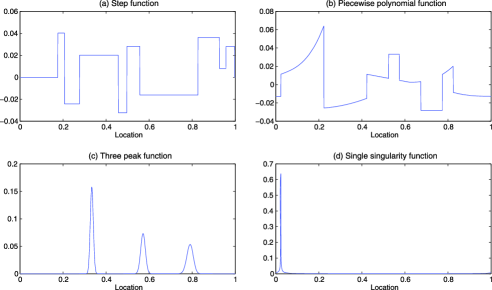
Figure 1: Four test vectors in the original domain: values at $p=2048$ equispaced points on $[0,1]$ of four test functions. (a) step: step function, (b) poly: piecewise polynomial function, (c) peak: three-peak function and (d) sing: single singularity function.

Before applying any sparse PCA method, we transform the observed data vectors into the wavelet domain using the Symmlet 8 basis mall09 , and scale all the observations by $\widehat{\sigma}$ with $\widehat{\sigma}^{2}$ given in (5). The multi-resolution plots of wavelet coefficients of the test vectors are shown in Figure 2. In the wavelet domain, the four vectors exhibits different levels of sparsity, with step the least sparse, and sing the most.

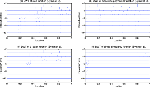
Figure 2: Discrete wavelet transform of the four test vectors in Figure 1. In each plot, the length of each stick is proportional to the magnitude of the Symmlet 8 wavelet coefficient at the given location and resolution level.

Table 1 compares the average loss of subspace estimation over $100$ runs for each spike value and each test vector by Algorithm 1 (ITSPCA) with several existing methods: augmented sparse PCA (AUGSPCA) pajo07 , correlation augmented sparse PCA (CORSPCA) nadl09 and diagonal thresholding sparse PCA (DTSPCA) given in Algorithm 2. For ITSPCA, we computed $\widehat{Q}{}^{(0)}$ by Algorithm 2. $\alpha_{n}$ and $\gamma_{n1}$ are specified by (7) and (8) with $\alpha=3$ and $\gamma=1.5$. These values are smaller than those in theoretical results, but lead to better numerical performance. We stop iterating once $L(\operatorname{ran}(\widehat{Q}{}^{(k)}),\operatorname{ran}(\widehat{Q}{}^{(k+1)}))\leq n^{-2}$. Parameters in competing algorithms are all set to the values recommended by their authors.

Table 1: Comparison of sparse PCA methods in single spike settings: average loss in estimation and size of selected feature set

		ITSPCA		AUGSPCA		CORSPCA		DTSPCA
Test vector	$\bolds{\lambda_{1}^{2}}$	Loss	Size	Loss	Size	Loss	Size	Loss	Size
Step	$100$	$0.0061$	$114.2$	$0.0096$	$96.5$	$0.0055$	$120.1$	$0.0275$	$66.6$
	$25$	$0.0224$	$76.3$	$0.0362$	$55.4$	$0.0236$	$73.9$	$0.0777$	$38.3$
	$10$	$0.0470$	$53.4$	$0.0710$	$37.4$	$0.0551$	$45.9$	$0.1494$	$24.1$
	$5$	$0.0786$	$45.5$	$0.1370$	$23.7$	$0.1119$	$28.7$	$0.2203$	$17.1$
	$2$	$0.1921$	$25.4$	$0.3107$	$11.4$	$0.3846$	$15.2$	$0.4518$	$9.7$
Poly	$100$	$0.0060$	$83.1$	$0.0088$	$66.5$	$0.0051$	$92.0$	$0.0191$	$49.2$
	$25$	$0.0175$	$52.4$	$0.0254$	$41.4$	$0.0173$	$53.1$	$0.0540$	$28.7$
	$10$	$0.0346$	$38.7$	$0.0527$	$27.5$	$0.0404$	$34.0$	$0.0959$	$20.5$
	$5$	$0.0588$	$30.7$	$0.0844$	$20.2$	$0.0684$	$24.6$	$0.1778$	$14.0$
	$2$	$0.1317$	$20.0$	$0.2300$	$10.3$	$0.2155$	$16.3$	$0.3370$	$8.1$
Peak	$100$	$0.0019$	$45.7$	$0.0032$	$39.6$	$0.0016$	$51.2$	$0.0075$	$32.8$
	$25$	$0.0071$	$34.1$	$0.0099$	$29.9$	$0.0069$	$35.2$	$0.0226$	$24.3$
	$10$	$0.0158$	$28.0$	$0.0222$	$23.8$	$0.0165$	$27.3$	$0.0592$	$18.6$
	$5$	$0.0283$	$24.7$	$0.0449$	$19.6$	$0.0320$	$22.5$	$0.1161$	$14.1$
	$2$	$0.0927$	$20.8$	$0.1887$	$9.9$	$0.1176$	$14.6$	$0.2702$	$8.8$
Sing	$100$	$0.0016$	$38.0$	$0.0025$	$33.2$	$0.0014$	$43.6$	$0.0070$	$26.3$
	$25$	$0.0068$	$27.1$	$0.0095$	$23.1$	$0.0060$	$31.8$	$0.0237$	$17.5$
	$10$	$0.0161$	$20.3$	$0.0233$	$16.6$	$0.0154$	$20.9$	$0.0377$	$13.6$
	$5$	$0.0279$	$17.3$	$0.0372$	$13.2$	$0.0313$	$15.2$	$0.0547$	$12.7$
	$2$	$0.0631$	$15.2$	$0.0792$	$10.9$	$0.0652$	$13.0$	$0.2025$	$8.8$

From Table 1, ITSPCA and CORSPCA outperform the other two methods in all settings. Between the two, CORSPCA only wins by small margins when the spike values are large. Otherwise, ITSPCA wins, sometimes with large margins. For the same algorithm at the same spike value, the sparser the signal, the smaller the estimation error.

Table 1 also presents the average sizes of the sets of selected coordinates. While all methods yield sparse PC loadings, AUGSPCA and DTSPCA seem to select too few coordinates, and thus introduce too much bias. ITSPCA and CORSPCA apparently result in a better bias-variance tradeoff.

5.2 Multiple spike settings

Next, we simulated data vectors using model (6) with ${\bar{m}}=4$. The $q_{j}$ vectors are taken to be the four test vectors used in single spike settings, in the same order as in Figure 1, up to orthonormalization. We tried four different configurations of the spike values $(\lambda_{1}^{2},\ldots,\lambda_{4}^{2})$, as specified in the first column of Table 2. For each configuration of spike values, the dimension is $p=2048$, and the sample size is $n=1024$.

Table 2: Comparison of sparse PCA methods in multiple spike settings: average loss in estimation

		$\bolds{L(\mathcal{P}_{m},\widehat{\mathcal{P}}_{m})}$
$\bolds{(\lambda_{1}^{2},\lambda_{2}^{2},\lambda_{3}^{2},\lambda_{4}^{2})}$	$\bolds{m}$	ITSPCA	AUGSPCA	CORSPCA	DTSPCA
$(100,75,50,25)$	$1$	$0.0216$	$0.0260$	$0.0240$	$0.0378$
	$2$	$0.0180$	$0.0213$	$0.0214$	$0.0308$
	$3$	$0.0094$	$0.0129$	$0.0126$	$0.0234$
	$4$	$0.0087$	$0.0122$	$0.0181$	$0.0235$
$(60,55,50,45)$	$1$	$0.3100$	$0.2588$	$0.2548$	$0.2831$
	$2$	$0.2675$	$0.2045$	$0.2095$	$0.2349$
	$3$	$0.1844$	$0.1878$	$0.1872$	$0.1968$
	$4$	$0.0157$	$0.0203$	$0.0178$	$0.0333$
$(30,27,25,22)$	$1$	$0.3290$	$0.2464$	$0.2495$	$0.2937$
	$2$	$0.3147$	$0.2655$	$0.2882$	$0.3218$
	$3$	$0.1740$	$0.1662$	$0.1708$	$0.1821$
	$4$	$0.0270$	$0.0342$	$0.0338$	$0.0573$
$(30,20,10,5)$	$1$	$0.0268$	$0.0392$	$0.0380$	$0.0658$
	$2$	$0.0237$	$0.0353$	$0.0391$	$0.0605$
	$3$	$0.0223$	$0.0336$	$0.0372$	$0.0599$
	$4$	$0.0298$	$0.0414$	$0.0717$	$0.0638$

For each simulated dataset, we estimate $\mathcal{P}_{m}$ for $m=1,2,3$ and $4$. The last four columns of Table 2 present the losses in estimating subspaces, averaged over $100$ runs, using the same sparse PCA methods as in single spike settings. For ITSPCA, we set the thresholds $\{\gamma_{nj},j=1,\ldots,4\}$ as in (8) with $\gamma=1.5$. All other implementation details are the same. Again, we used recommended values for parameters in all other competing methods.

The simulation results reveal two interesting phenomena. First, when the spikes are relatively well separated (the first and the last blocks of Table 2), all methods yield decent estimators of $\mathcal{P}_{m}$ for all values of $m$, which implies that the individual eigenvectors are also estimated well. In this case, ITSPCA always outperforms the other three competing methods. Second, when the spikes are not so well separated (the middle two blocks, with $m=1,2$ or $3$), no method leads to decent subspace estimator. However, all methods give reasonable estimators for $\mathcal{P}_{4}$ because $\lambda_{4}^{2}$ in both cases are well above $0$. This implies that, under such settings, we fail to recover individual eigenvectors, but we can still estimate $\mathcal{P}_{4}$ well. ITSPCA again gives the smallest average losses. In all configurations, the estimated number of spikes $\widehat{\bar{m}}$ in (17) and the data-based choice of $m$ in (20) with $\bar{\kappa}=15$ consistently picked $m=\widehat{\bar{m}}=4$ in all simulated datasets. Therefore, we are always led to estimating the “right” subspace $\mathcal{P}_{4}$, and ITSPCA performs favorably over the competing methods.

In summary, simulations under multiple spike settings not only demonstrate the competitiveness of Algorithm 1, but also suggest: [(2)]

The quality of principal subspace estimation depends on the gap between successive eigenvalues, in addition to the sparsity of eigenvectors;

Focusing on individual eigenvectors can be misleading for the purpose of finding low-dimensional projections.

6 Proof

This section is devoted to the proofs of Theorems 3.2 and 3.3. We state the main ideas in Section 6.1 and divide the proof into three major steps, which are then completed in sequel in Sections 6.2–6.4. Others results in Section 3.4 are proved in the supplementary material supp .

6.1 Main ideas and outline of proof

The proof is based on an oracle sequence approach, the main ideas of which are as follows. First, assuming oracle knowledge of the set $H$, we construct a sequence of $p\times m$ orthonormal matrices $\{\widehat{Q}{}^{(k),\mathrm{o}},k\geq 0\}$. Then we study how fast the sequence converges, and how well each associated column subspace approximates the principal subspace $\mathcal{P}_{m}$ of interest. Finally, we show that, with high probability, the first $K_{s}$ terms of the oracle sequence is exactly the sequence $\{\widehat{Q}{}^{(k)},0\leq k\leq K_{s}\}$ obtained by Algorithm 1. The actual estimating sequence thus inherits from the oracle sequence various properties in terms of estimation error and number of steps needed to achieve the desired error rate. The actual sequence mimics the oracle because the thresholding step forces it to only consider the high signal coordinates in $H$.

In what follows, we first construct the oracle sequence and then lay out a road map of the proof. Here and after, we use an extra superscript “$\mathrm{o}$” to indicate oracle quantities. For example, $\widehat{Q}{}^{(k),\mathrm{o}}$ denotes the $k$th orthonormal matrix in the oracle sequence.

Construction of the oracle sequence

First, we construct $\widehat{Q}{}^{(0),\mathrm{o}}$ using an oracle version of Algorithm 2, where the set $B$ is replaced by its oracle version $B^{\mathrm{o}}=B\cap H$. This ensures that $\widehat{Q}{}^{(0),\mathrm{o}}_{L\cdot}=0$.

To construct the rest of the sequence, suppose that the $p$ features are organized (after reordering) in such a way that those in $H$ always have smaller indices than those in $L$, and that within $H$, those in $B^{\mathrm{o}}$ precede those not. Define the oracle sample covariance matrix

$$S^{\mathrm{o}}=\left[\matrix{S_{HH}&0\cr 0&I_{LL}}\right].$$ (21)

Here, $I_{LL}$ is the identity matrix of dimension $\operatorname{card}(L)$. Then, the matrices $\{\widehat{Q}{}^{(k),\mathrm{o}},k\geq 0\}$ are obtained via an oracle version of Algorithm 1, in which the initial matrix is $\widehat{Q}{}^{(0),\mathrm{o}}$, and $S$ is replaced by $S^{\mathrm{o}}$.

Remark 6.1.

This formal construction does not guarantee that $\widehat{Q}{}^{(k),\mathrm{o}}$ has full column rank or that $\widehat{Q}{}^{(k),\mathrm{o}}_{L\cdot}=0$ for all $k$. Later, Lemma 6.3, Proposition 6.1 and Lemma 6.4 show that these statements are true with high probability for all $k\leq K_{s}$.

Major steps of the proof

In the $k$th iteration of the oracle Algorithm 1, denote the matrices obtained after multiplication and thresholding by

$$T^{(k),\mathrm{o}} = S^{\mathrm{o}}\widehat{Q}{}^{(k-1),\mathrm{o}}=\bigl{(}t_{\nu j}^{(k),\mathrm{o}}\bigr{)}\quad\mbox{and}$$

$$\widehat{T}{}^{(k),\mathrm{o}} = \bigl{(}\widehat{t}_{\nu j}^{(k),\mathrm{o}}\bigr{)}\qquad\mbox{with $\widehat{t}_{\nu j}^{(k),\mathrm{o}}=\eta\bigl{(}{t}_{\nu j}^{(k),\mathrm{o}},\gamma_{nj}\bigr{)}$.}$$

Further denote the QR factorization of $\widehat{T}{}^{(k),\mathrm{o}}$ by $\widehat{T}{}^{(k),\mathrm{o}}=\widehat{Q}{}^{(k),\mathrm{o}}\widehat{R}{}^{(k),\mathrm{o}}$. Last but not least, let $\widehat{\mathcal{P}}_{m}^{(k),\mathrm{o}}=\operatorname{ran}(\widehat{Q}{}^{(k),\mathrm{o}})$.

A joint proof of Theorems 3.2 and 3.3 can then be completed by the following three major steps: [(3)]

show that the principal subspace of $S^{\mathrm{o}}$ with dimension $m$, denoted by $\widehat{\mathcal{P}}_{m}^{\mathrm{o}}$, satisfies the error bound in (16) for estimating $\mathcal{P}_{m}$;

show that for $K$ in (15), $K_{s}\in[K,2K]$ and that the approximation error of $\widehat{\mathcal{P}}_{m}^{(k),\mathrm{o}}$ to $\widehat{\mathcal{P}}_{m}^{\mathrm{o}}$ for all $k\geq K$ also satisfies the bound in (16);

show that $\widehat{Q}_{L\cdot}^{(k),\mathrm{o}}=0$ for all $k\leq 2K$, and that the oracle and the actual estimating sequences are identical up to $2K$ iterations. In each step, we only need the result to hold with high probability. By the triangle inequality, steps 1 and 2 imply that the error of $\widehat{\mathcal{P}}_{m}^{{(K_{s})},\mathrm{o}}$ in estimating $\mathcal{P}_{m}$ satisfies (16). Step 3 shows this is also the case for the actual estimator $\widehat{\mathcal{P}}_{m}^{{(K_{s})}}$. It also implies the correct exclusion property in Theorem 3.3.

In what follows, we complete the three steps in Sections 6.2–6.4.

6.2 Principal subspace of $S^{\mathrm{o}}$

To study how well the principal subspace of $S^{\mathrm{o}}$ approximates $\mathcal{P}_{m}$, we break into a “bias” part and a “variance” part.

Consider the “bias” part first. Define the oracle covariance matrix

$$\Sigma^{\mathrm{o}}=\left[\matrix{\Sigma_{HH}&0\cr 0&I_{LL}}\right],$$ (23)

which is the expected value of $S^{\mathrm{o}}$. The following lemma gives the error of the principal subspace of $\Sigma^{\mathrm{o}}$ in approximating $\mathcal{P}_{m}$, which could be regarded as the “squared bias” induced by feature selection.

Lemma 6.1

Let the eigenvalues of $\Sigma^{\mathrm{o}}$ be $\ell_{1}^{\mathrm{o}}\geq\cdots\geq\ell_{\bar{m}}^{\mathrm{o}}\geq\cdots\geq 0$ and $\{q_{1}^{\mathrm{o}},\ldots,q_{\bar{m}}^{\mathrm{o}}\}$ be a set of first $\bar{m}$ eigenvectors. Denote $Q^{\mathrm{o}}=[q_{1}^{\mathrm{o}},\ldots,q_{m}^{\mathrm{o}}]$. Then, uniformly over $\mathcal{F}_{n}$: [(2)]

$|\ell_{j}^{\mathrm{o}}-(\lambda_{j}^{2}+1)|/\lambda_{1}^{2}\to 0$ as $n\to\infty$, for $j=1,\ldots,\bar{m}+1$, with $\lambda_{\bar{m}+1}^{2}=0$;

for sufficiently large $n$, $Q^{\mathrm{o}}_{L\cdot}=0$ and for ${\mathcal{P}}^{\mathrm{o}}_{m}=\operatorname{ran}(Q^{\mathrm{o}})$, there exists a constant $C=C(m,r,\kappa)$, s.t. $L(\mathcal{P}_{m},\mathcal{P}^{\mathrm{o}}_{m})\leq CM_{n}\tau_{nm}^{2}$.

A proof is given in the supplementary material supp . Weyl’s theorem (stsu90 , Corollary 4.4.10) and Davis–Kahn’s $\sin\theta$ theorem daka70 are the key ingredients in the proof here, and also in the proofs of Lemmas 6.2 and 6.3. Here, claim (1) only requires Conditions GR and SP, but not the condition $\operatorname{AD}(m,\kappa)$.

Turn to the “variance” part. We check how well the principal subspace of $S^{\mathrm{o}}$ estimates $\mathcal{P}^{\mathrm{o}}$. Since $\Sigma^{\mathrm{o}}=\mathbb{E}[S^{\mathrm{o}}]$, the error here is analogous to “variance.”

Lemma 6.2

Let the eigenvalues of $S^{\mathrm{o}}$ be $\widehat{\ell}_{1}^{\mathrm{o}}\geq\cdots\geq\widehat{\ell}_{\bar{m}}^{\mathrm{o}}\geq\cdots\geq 0$ and $\{\widehat{q}_{1}^{\mathrm{o}},\ldots,\widehat{q}_{\bar{m}}^{\mathrm{o}}\}$ be a set of first $\bar{m}$ eigenvectors. Denote $\widehat{Q}{}^{\mathrm{o}}=[\widehat{q}_{1}^{\mathrm{o}},\ldots,\widehat{q}_{m}^{\mathrm{o}}]$. Then, uniformly over $\mathcal{F}_{n}$, with probability at least $1-C_{0}p_{n}^{-2}$: [(2)]

$|\widehat{\ell}_{j}^{\mathrm{o}}-\ell_{j}^{\mathrm{o}}|/\lambda_{1}^{2}\to 0$ as $n\to\infty$, for $j=1,\ldots,\bar{m}+1$;

for sufficiently large $n$, $\widehat{Q}{}^{\mathrm{o}}_{L\cdot}=0$, and for $\widehat{\mathcal{P}}{}^{\mathrm{o}}_{m}=\operatorname{ran}(\widehat{Q}{}^{\mathrm{o}})$, there exist constants $C_{1}=C_{1}(m,r,\kappa)$ and $C_{2}$, s.t.

$$L\bigl{(}{\mathcal{P}}^{\mathrm{o}}_{m},\widehat{\mathcal{P}}{}^{\mathrm{o}}_{m}\bigr{)}\leq C_{1}M_{n}\tau_{nm}^{2}/\log(p_{n})+C_{2}\varepsilon_{nm}^{2}.$$

A proof is given in the supplementary material supp . Again, claim (1) does not require the condition $\operatorname{AD}(m,\kappa)$. By the triangle inequality, the above two lemmas imply the error in estimating $\mathcal{P}_{m}$ with $\widehat{\mathcal{P}}_{m}^{\mathrm{o}}$ satisfies the bound in (16).

6.3 Properties of the oracle sequence

In step 2, we study properties of the oracle sequence. For $K$ in (15), the goal is to show that, with high probability, for all $k\geq K$, the error of the oracle subspace estimator $\widehat{\mathcal{P}}_{m}^{(k),\mathrm{o}}$ in approximating $\widehat{\mathcal{P}}_{m}^{\mathrm{o}}$ satisfies in (16). To this end, characterization of the oracle sequence evolution in Proposition 6.1 below plays the key role.

The initial point

We start with the initial point. Let

$$\rho={\widehat{\ell}{}^{\mathrm{o}}_{m+1}}/{\widehat{\ell}{}^{\mathrm{o}}_{m}}$$ (24)

denote the ratio between the $(m+1)$th and the $m$th largest eigenvalues of $S^{\mathrm{o}}$. The following lemma shows that $\widehat{Q}{}^{(0),\mathrm{o}}$ is orthonormal and is a good initial point for (oracle) Algorithm 1.

Lemma 6.3

Uniformly over $\mathcal{F}_{n}$, with probability at least $1-C_{0}p_{n}^{-2}$: [(4)]

$B^{\mathrm{o}}=B$;

$|\ell_{j}(S_{B^{\mathrm{o}}B^{\mathrm{o}}})\vee 1-\widehat{\ell}_{j}^{\mathrm{o}}|/\lambda_{1}^{2}\to 0$ as $n\to\infty$, for $j=1,\ldots,\bar{m}+1$;

for sufficiently large $n$, $\widehat{Q}{}^{(0),\mathrm{o}}$ has full column rank, and $L(\widehat{\mathcal{P}}{}^{\mathrm{o}}_{m},\widehat{\mathcal{P}}_{m}^{(0),\mathrm{o}})\leq(1-\rho)^{2}/5$;

for sufficiently large $n$, $K_{s}\in[K,2K]$.

A proof is given in the supplementary material supp . Here, claims (1) and (2) do not require the condition $\operatorname{AD}(m,\kappa)$. In claim (3), the bound $(1-\rho)^{2}/5$ is much larger than that in (16). For instance, if $\lambda_{m}^{2}+1\asymp\lambda_{m}^{2}-\lambda_{m+1}^{2}$, Lemmas 6.1 and 6.2 imply that $(1-\rho^{2})/5\asymp 1$ with high probability.

Claims (1) and (2) here, together with claims (1) of Lemmas 6.1 and 6.2, lead to the following result on consistent estimation of $\lambda_{1}^{2}/(\lambda_{j}^{2}-\lambda_{j+1}^{2})$ and $\lambda_{j}^{2}$, the proof of which is given in the supplementary material supp .

Corollary 6.1

Suppose Conditions GR and SP hold, and let $\ell^{B}_{j}=\ell_{j}(S_{BB})\vee 1$. For $1\leq j\leq\bar{m}$, if $\lim_{n\to\infty}\lambda_{1}^{2}/(\lambda_{j}^{2}-\lambda_{j+1}^{2})<\infty$, then

$$\lim_{n\to\infty}\frac{(\ell^{B}_{1}-1)/(\ell^{B}_{j}-\ell^{B}_{j+1})}{\lambda_{1}^{2}/(\lambda_{j}^{2}-\lambda_{j+1}^{2})}=1\qquad\mbox{a.s.}$$

Otherwise, $\lim_{n\to\infty}(\ell^{B}_{1}-1)/(\ell^{B}_{j}-\ell^{B}_{j+1})=\lim_{n\to\infty}\lambda_{1}^{2}/(\lambda_{j}^{2}-\lambda_{j+1}^{2})=\infty$, a.s.

If further the condition $\operatorname{AD}(m,\kappa)$ holds for some $m\leq\bar{m}$ and $\kappa>0$, then $\lim_{n\to\infty}(\ell^{B}_{j}-1)/\lambda_{j}^{2}=1$, a.s., for $1\leq j\leq m$.

Evolution of the oracle sequence

Next, we study the evolution of the oracle sequence. Let ${\theta}^{(k)}\in[0,\pi/2]$ be the largest canonical angle between the subspaces $\widehat{\mathcal{P}}{}^{\mathrm{o}}_{m}$ and $\widehat{\mathcal{P}}_{m}^{(k),\mathrm{o}}$. By the discussion after (3), we have

$$\sin^{2}{\theta}^{(k)}=L\bigl{(}\widehat{\mathcal{P}}_{m}^{\mathrm{o}},\widehat{\mathcal{P}}_{m}^{(k),\mathrm{o}}\bigr{)}.$$ (25)

The following proposition describes the evolution of ${\theta}^{(k)}$ over iterations.

Proposition 6.1

Let $n$ be sufficiently large. On the event such that the conclusions of Lemmas 6.1–6.3 hold, uniformly over $\mathcal{F}_{n}$, for all $k\geq 1$: [(2)]

$\widehat{Q}{}^{(k),\mathrm{o}}$ is orthonormal, and ${\theta}^{(k)}$ satisfies

$$\sin{\theta}^{(k)}\leq\rho\tan{\theta}^{(k-1)}+\omega\sec{\theta}^{(k-1)},$$ (26)

where $\omega=(\widehat{\ell}_{m}^{\mathrm{o}})^{-1}[\operatorname{card}(H)\sum_{j=1}^{m}\gamma_{nj}^{2}]^{1/2}$;

for any $a\in(0,1/2]$, if

$$\sin^{2}{\theta}^{(k-1)}\leq{1.01(1-a)^{-2}\omega^{2}}{(1-\rho)^{-2}},$$ (27)

then so is $\sin^{2}{{\theta}^{(k)}}$. Otherwise,

$$\sin^{2}{\theta}^{(k)}/\sin^{2}{\theta}^{(k-1)}\leq\bigl{[}1-a(1-\rho)\bigr{]}^{2}.$$ (28)

A proof is given in the supplementary material supp , the key ingredient of which is Wedin’s $\sin\theta$ theorem for singular subspaces wedi72 . The recursive inequality (26) characterizes the evolution of the angles ${\theta}^{(k)}$, and hence of the oracle subspace $\widehat{\mathcal{P}}_{m}^{(k),\mathrm{o}}$. It is the foundation of claim (2) in the current proposition and of Proposition 6.2 below.

By (25), inequality (28) gives the rate at which the approximation error $L(\widehat{\mathcal{P}}_{m}^{\mathrm{o}},\widehat{\mathcal{P}}_{m}^{(k),\mathrm{o}})$ decreases. For a given $a\in(0,1/2]$, the rate is maintained until the error becomes smaller than $1.01(1-a)^{-2}\omega^{2}(1-\rho)^{-2}$. Then the error continues to decrease, but at a slower rate, say, with $a$ replaced by $a/2$ in (28), until (27) is satisfied with $a$ replaced by $a/2$. The decrease continues at slower and slower rate in this fashion until the approximation error falls into the interval $[0,{1.01\omega^{2}}/{(1-\rho)^{2}}]$, and remains inside thereafter.

Together with Lemma 6.3, Proposition 6.1 also justifies the previous claim that elements of the oracle sequence are orthonormal with high probability.

Convergence

Finally, we study how fast the oracle sequence converges to a stable subspace estimator, and how good this estimator is.

To define convergence of the subspace sequence $\{\widehat{\mathcal{P}}_{m}^{(k),\mathrm{o}},k\geq 0\}$, we first note that $1.01\omega^{2}/(1-\rho)^{2}$ is almost the smallest possible value of $L(\widehat{\mathcal{P}}_{m}^{\mathrm{o}},\widehat{\mathcal{P}}_{m}^{(k),\mathrm{o}})$ that (26) could imply. Indeed, when $\sin{\theta}^{(k)}$ converges and is small, we have $\sin{\theta}^{(k)}\approx\sin{\theta}^{(k-1)}$, and $\cos{\theta}^{(k)}\approx 1$. Consequently, (26) reduces to

$$\sin{\theta}^{(k)}\leq\bigl{(}\rho\sin{\theta}^{(k)}+\omega\bigr{)}\bigl{(}1+o(1)\bigr{)}.$$

So, $L(\widehat{\mathcal{P}}_{m}^{\mathrm{o}},\widehat{\mathcal{P}}_{m}^{(k),\mathrm{o}})=\sin^{2}{\theta}^{(k)}\leq(1+o(1))\omega^{2}/(1-\rho)^{2}$. In addition, Lemma 6.2 suggests that we can stop the iteration as soon as $L(\widehat{\mathcal{P}}_{m}^{\mathrm{o}},\widehat{\mathcal{P}}_{m}^{(k),\mathrm{o}})$ becomes smaller than a constant multiple of $\varepsilon_{nm}^{2}$, for we always get an error of order $O(\varepsilon_{nm}^{2})$ for estimating $\mathcal{P}_{m}$, even if we use $\widehat{\mathcal{P}}_{m}^{\mathrm{o}}$ directly. In observation of both aspects, we say that $\widehat{\mathcal{P}}_{m}^{(k),\mathrm{o}}$ has converged if

$$L\bigl{(}\widehat{\mathcal{P}}_{m}^{\mathrm{o}},\widehat{\mathcal{P}}_{m}^{(k),\mathrm{o}}\bigr{)}\leq\max\biggl{\{}\frac{1.01}{(1-n^{-1})^{2}}\frac{\omega^{2}}{(1-\rho)^{2}},\varepsilon_{nm}^{2}\biggr{\}}.$$ (29)

On the event that conclusions of Lemmas 6.1–6.3 hold, we have $\omega^{2}/(1-\rho)^{2}=O(M_{n}\tau_{nm}^{2})$. Under definition (29), for $K$ in (15), the following proposition shows that it takes $K$ iterations for the oracle sequence to converge, and for all $k\geq K$, the error of approximating $\widehat{\mathcal{P}}_{m}^{\mathrm{o}}$ by $\widehat{\mathcal{P}}_{m}^{(k),\mathrm{o}}$ satisfies (16).

Proposition 6.2

For sufficiently large $n$, on the event such that the conclusions of Lemmas 6.1–6.3 hold, uniformly over $\mathcal{F}_{n}$, it takes at most $K$ steps for the oracle sequence to converge. In addition, there exist constants $C_{1}=C_{1}(\gamma,r,m,\kappa)$ and $C_{2}$, such that for all $k\geq K$,

$$\sup_{\mathcal{F}_{n}}L\bigl{(}\widehat{\mathcal{P}}_{m}^{\mathrm{o}},\widehat{\mathcal{P}}_{m}^{(k),\mathrm{o}}\bigr{)}\leq C_{1}M_{n}\tau_{nm}^{2}+C_{2}\varepsilon_{nm}^{2}.$$ (30)

A proof is given in the supplementary material supp , and this completes step 2.

6.4 Proof of main results

We now prove the properties of the actual estimating sequence. The proof relies on the following lemma, which shows the actual and the oracle sequences are identical up to $2K$ iterations.

Lemma 6.4

For sufficiently large $n$, with probability at least $1-C_{0}p_{n}^{-2}$, for all $k\leq 2K$, we have $\widehat{Q}{}^{(k),\mathrm{o}}_{L\cdot}=0$, $\widehat{Q}{}^{(k)}=\widehat{Q}{}^{(k),\mathrm{o}}$, and hence $\widehat{\mathcal{P}}_{m}^{(k)}=\widehat{\mathcal{P}}_{m}^{(k),\mathrm{o}}$.

A proof is given in the supplementary material supp , and this completes step 3.

We now prove Theorems 3.2 and 3.3 by showing that the actual sequence inherits the desired properties from the oracle sequence. Since Theorem 3.1 is a special case of Theorem 3.2, we do not give a separate proof.

Proof of Theorem 3.2 Note that the event on which the conclusions of Lemmas 6.1–6.4 hold has probability at least $1-C_{0}p_{n}^{-2}$. On this event,

$$L\bigl{(}\mathcal{P}_{m},\widehat{\mathcal{P}}_{m}^{{(K_{s})}}\bigr{)} = L\bigl{(}\mathcal{P}_{m},\widehat{\mathcal{P}}_{m}^{{(K_{s})},\mathrm{o}}\bigr{)}$$

$$\leq \bigl{[}L^{{1/2}}\bigl{(}\mathcal{P}_{m},\mathcal{P}_{m}^{\mathrm{o}}\bigr{)}+L^{{1/2}}\bigl{(}\mathcal{P}_{m}^{\mathrm{o}},\widehat{\mathcal{P}}_{m}^{\mathrm{o}}\bigr{)}+L^{{1/2}}\bigl{(}\widehat{\mathcal{P}}_{m}^{\mathrm{o}},\widehat{\mathcal{P}}_{m}^{{(K_{s})},\mathrm{o}}\bigr{)}\bigr{]}^{2}$$

$$\leq C\bigl{[}L\bigl{(}\mathcal{P}_{m},\mathcal{P}_{m}^{\mathrm{o}}\bigr{)}+L\bigl{(}\mathcal{P}_{m}^{\mathrm{o}},\widehat{\mathcal{P}}_{m}^{\mathrm{o}}\bigr{)}+L\bigl{(}\widehat{\mathcal{P}}_{m}^{\mathrm{o}},\widehat{\mathcal{P}}_{m}^{{(K_{s})},\mathrm{o}}\bigr{)}\bigr{]}$$

$$\leq C_{1}M_{n}\tau_{nm}^{2}+C_{2}\varepsilon_{nm}^{2}.$$

Here, the first equality comes from Lemma 6.4. The first two inequalities result from the triangle inequality and Jensen’s inequality, respectively. Finally, the last inequality is obtained by noting that $K_{s}\in[K,2K]$ and by replacing all the error terms by their corresponding bounds in Lemmas 6.1, 6.2 and Proposition 6.2.

Proof of Theorem 3.3 Again, we consider the event on which the conclusions of Lemmas 6.1–6.4 hold. Then Lemma 6.4 directly leads to the conclusion that $\widehat{Q}{}^{(k)}_{L\cdot}=\widehat{Q}{}^{(k),\mathrm{o}}_{L\cdot}=0$, for all $0\leq k\leq K_{s}\leq 2K$.

References

- (1) {barticle}[mr] \bauthor\bsnmAmini, \bfnmArash A.\binitsA. A. and \bauthor\bsnmWainwright, \bfnmMartin J.\binitsM. J. (\byear2009). \btitleHigh-dimensional analysis of semidefinite relaxations for sparse principal components. \bjournalAnn. Statist. \bvolume37 \bpages2877–2921. \biddoi=10.1214/08-AOS664, issn=0090-5364, mr=2541450 \bptokimsref \endbibitem
- (2) {barticle}[mr] \bauthor\bsnmAnderson, \bfnmT. W.\binitsT. W. (\byear1963). \btitleAsymptotic theory for principal component analysis. \bjournalAnn. Math. Statist. \bvolume34 \bpages122–148. \bidissn=0003-4851, mr=0145620 \bptokimsref \endbibitem
- (3) {barticle}[mr] \bauthor\bsnmd’Aspremont, \bfnmAlexandre\binitsA., \bauthor\bsnmEl Ghaoui, \bfnmLaurent\binitsL., \bauthor\bsnmJordan, \bfnmMichael I.\binitsM. I. and \bauthor\bsnmLanckriet, \bfnmGert R. G.\binitsG. R. G. (\byear2007). \btitleA direct formulation for sparse PCA using semidefinite programming. \bjournalSIAM Rev. \bvolume49 \bpages434–448 (electronic). \biddoi=10.1137/050645506, issn=0036-1445, mr=2353806 \bptokimsref \endbibitem
- (4) {barticle}[mr] \bauthor\bsnmDavis, \bfnmChandler\binitsC. and \bauthor\bsnmKahan, \bfnmW. M.\binitsW. M. (\byear1970). \btitleThe rotation of eigenvectors by a perturbation. III. \bjournalSIAM J. Numer. Anal. \bvolume7 \bpages1–46. \bidissn=0036-1429, mr=0264450 \bptokimsref \endbibitem
- (5) {barticle}[mr] \bauthor\bsnmDonoho, \bfnmDavid L.\binitsD. L. (\byear1993). \btitleUnconditional bases are optimal bases for data compression and for statistical estimation. \bjournalAppl. Comput. Harmon. Anal. \bvolume1 \bpages100–115. \biddoi=10.1006/acha.1993.1008, issn=1063-5203, mr=1256530 \bptokimsref \endbibitem
- (6) {barticle}[mr] \bauthor\bsnmFan, \bfnmJianqing\binitsJ. and \bauthor\bsnmLi, \bfnmRunze\binitsR. (\byear2001). \btitleVariable selection via nonconcave penalized likelihood and its oracle properties. \bjournalJ. Amer. Statist. Assoc. \bvolume96 \bpages1348–1360. \biddoi=10.1198/016214501753382273, issn=0162-1459, mr=1946581 \bptokimsref \endbibitem
- (7) {bbook}[mr] \bauthor\bsnmGolub, \bfnmGene H.\binitsG. H. and \bauthor\bsnmVan Loan, \bfnmCharles F.\binitsC. F. (\byear1996). \btitleMatrix Computations, \bedition3rd ed. \bpublisherJohns Hopkins Univ. Press, \blocationBaltimore, MD. \bidmr=1417720 \bptokimsref \endbibitem
- (8) {barticle}[auto:STB—2013/04/03—07:24:31] \bauthor\bsnmHotelling, \bfnmH.\binitsH. (\byear1933). \btitleAnalysis of a complex of statistical variables into principal components. \bjournalJ. Educ. Psychol. \bvolume24 \bpages417–441, 498–520. \bptokimsref \endbibitem
- (9) {barticle}[auto:STB—2013/04/03—07:24:31] \bauthor\bsnmHoyle, \bfnmD. C.\binitsD. C. and \bauthor\bsnmRattray, \bfnmM.\binitsM. (\byear2004). \btitlePrincipal-component-analysis eigenvalue spectra from data with symmetry-breaking structure. \bjournalPhys. Rev. E (3) \bvolume69 \bpages026124. \bptokimsref \endbibitem
- (10) {barticle}[mr] \bauthor\bsnmJohnstone, \bfnmIain M.\binitsI. M. (\byear2001). \btitleOn the distribution of the largest eigenvalue in principal components analysis. \bjournalAnn. Statist. \bvolume29 \bpages295–327. \biddoi=10.1214/aos/1009210544, issn=0090-5364, mr=1863961 \bptokimsref \endbibitem
- (11) {barticle}[mr] \bauthor\bsnmJohnstone, \bfnmIain M.\binitsI. M. and \bauthor\bsnmLu, \bfnmArthur Yu\binitsA. Y. (\byear2009). \btitleOn consistency and sparsity for principal components analysis in high dimensions. \bjournalJ. Amer. Statist. Assoc. \bvolume104 \bpages682–693. \biddoi=10.1198/jasa.2009.0121, issn=0162-1459, mr=2751448 \bptokimsref \endbibitem
- (12) {barticle}[mr] \bauthor\bsnmJolliffe, \bfnmIan T.\binitsI. T., \bauthor\bsnmTrendafilov, \bfnmNickolay T.\binitsN. T. and \bauthor\bsnmUddin, \bfnmMudassir\binitsM. (\byear2003). \btitleA modified principal component technique based on the LASSO. \bjournalJ. Comput. Graph. Statist. \bvolume12 \bpages531–547. \biddoi=10.1198/1061860032148, issn=1061-8600, mr=2002634 \bptokimsref \endbibitem
- (13) {barticle}[mr] \bauthor\bsnmJung, \bfnmSungkyu\binitsS. and \bauthor\bsnmMarron, \bfnmJ. S.\binitsJ. S. (\byear2009). \btitlePCA consistency in high dimension, low sample size context. \bjournalAnn. Statist. \bvolume37 \bpages4104–4130. \biddoi=10.1214/09-AOS709, issn=0090-5364, mr=2572454 \bptokimsref \endbibitem
- (14) {bmisc}[mr] \bauthor\bsnmLu, \bfnmArthur Yu\binitsA. Y. (\byear2002). \bhowpublishedSparse principal component analysis for functional data. Ph.D. thesis, Stanford Univ., Stanford, CA. \bidmr=2703298 \bptokimsref \endbibitem
- (15) {bmisc}[auto:STB—2013/04/03—07:24:31] \bauthor\bsnmMa, \bfnmZ.\binitsZ. (\byear2013). \bhowpublishedSupplement to “Sparse principal component analysis and iterative thresholding.” DOI:\doiurl10.1214/13-AOS1097SUPP. \bptokimsref \endbibitem
- (16) {bbook}[mr] \bauthor\bsnmMallat, \bfnmStéphane\binitsS. (\byear2009). \btitleA Wavelet Tour of Signal Processing: The Sparse Way. \bpublisherAcademic Press, \blocationNew York. \bptokimsref \endbibitem
- (17) {barticle}[mr] \bauthor\bsnmNadler, \bfnmBoaz\binitsB. (\byear2008). \btitleFinite sample approximation results for principal component analysis: A matrix perturbation approach. \bjournalAnn. Statist. \bvolume36 \bpages2791–2817. \biddoi=10.1214/08-AOS618, issn=0090-5364, mr=2485013 \bptokimsref \endbibitem
- (18) {barticle}[mr] \bauthor\bsnmNadler, \bfnmBoaz\binitsB. (\byear2009). \btitleDiscussion of “On consistency and sparsity for principal components analysis in high dimensions,” by I. M. Johnstone and A. Y. Lu. \bjournalJ. Amer. Statist. Assoc. \bvolume104 \bpages694–697. \biddoi=10.1198/jasa.2009.0147, issn=0162-1459, mr=2751449 \bptokimsref \endbibitem
- (19) {barticle}[mr] \bauthor\bsnmOnatski, \bfnmAlexei\binitsA. (\byear2012). \btitleAsymptotics of the principal components estimator of large factor models with weakly influential factors. \bjournalJ. Econometrics \bvolume168 \bpages244–258. \biddoi=10.1016/j.jeconom.2012.01.034, issn=0304-4076, mr=2923766 \bptokimsref \endbibitem
- (20) {bmisc}[mr] \bauthor\bsnmPaul, \bfnmDebashis\binitsD. (\byear2005). \bhowpublishedNonparametric estimation of principal components. Ph.D. thesis, Stanford Univ. \bidmr=2707156 \bptokimsref \endbibitem
- (21) {barticle}[mr] \bauthor\bsnmPaul, \bfnmDebashis\binitsD. (\byear2007). \btitleAsymptotics of sample eigenstructure for a large dimensional spiked covariance model. \bjournalStatist. Sinica \bvolume17 \bpages1617–1642. \bidissn=1017-0405, mr=2399865 \bptokimsref \endbibitem
- (22) {bmisc}[auto:STB—2013/04/03—07:24:31] \bauthor\bsnmPaul, \bfnmD.\binitsD. and \bauthor\bsnmJohnstone, \bfnmI. M.\binitsI. M. (\byear2007). \bhowpublishedAugmented sparse principal component analysis for high dimensional data. Available at arXiv:\arxivurl1202.1242v1. \bptokimsref \endbibitem
- (23) {barticle}[auto:STB—2013/04/03—07:24:31] \bauthor\bsnmPearson, \bfnmK.\binitsK. (\byear1901). \btitleOn lines and planes of closest fit to systems of points in space. \bjournalPhilos. Mag. Ser. 6 \bvolume2 \bpages559–572. \bptokimsref \endbibitem
- (24) {bbook}[mr] \bauthor\bsnmRamsay, \bfnmJ. O.\binitsJ. O. and \bauthor\bsnmSilverman, \bfnmB. W.\binitsB. W. (\byear2005). \btitleFunctional Data Analysis, \bedition2nd ed. \bpublisherSpringer, \blocationNew York. \bidmr=2168993 \bptokimsref \endbibitem
- (25) {barticle}[auto:STB—2013/04/03—07:24:31] \bauthor\bsnmReimann, \bfnmP.\binitsP., \bauthor\bparticleVan den \bsnmBroeck, \bfnmC.\binitsC. and \bauthor\bsnmBex, \bfnmG. J.\binitsG. J. (\byear1996). \btitleA Gaussian scenario for unsupervised learning. \bjournalJ. Phys. A \bvolume29 \bpages3521–3535. \bptokimsref \endbibitem
- (26) {bmisc}[auto:STB—2013/04/03—07:24:31] \bauthor\bsnmShen, \bfnmD.\binitsD., \bauthor\bsnmShen, \bfnmH.\binitsH. and \bauthor\bsnmMarron, \bfnmJ. S.\binitsJ. S. (\byear2011). \bhowpublishedConsistency of sparse PCA in high dimension, low sample size contexts. \bptokimsref \endbibitem
- (27) {barticle}[mr] \bauthor\bsnmShen, \bfnmHaipeng\binitsH. and \bauthor\bsnmHuang, \bfnmJianhua Z.\binitsJ. Z. (\byear2008). \btitleSparse principal component analysis via regularized low rank matrix approximation. \bjournalJ. Multivariate Anal. \bvolume99 \bpages1015–1034. \biddoi=10.1016/j.jmva.2007.06.007, issn=0047-259X, mr=2419336 \bptokimsref \endbibitem
- (28) {bbook}[mr] \bauthor\bsnmStewart, \bfnmG. W.\binitsG. W. and \bauthor\bsnmSun, \bfnmJi Guang\binitsJ. G. (\byear1990). \btitleMatrix Perturbation Theory. \bpublisherAcademic Press, \blocationBoston, MA. \bidmr=1061154 \bptokimsref \endbibitem
- (29) {bbook}[mr] \bauthor\bsnmTsay, \bfnmRuey S.\binitsR. S. (\byear2005). \btitleAnalysis of Financial Time Series, \bedition2nd ed. \bpublisherWiley, \blocationHoboken, NJ. \biddoi=10.1002/0471746193, mr=2162112 \bptokimsref \endbibitem
- (30) {barticle}[mr] \bauthor\bsnmUlfarsson, \bfnmMagnus O.\binitsM. O. and \bauthor\bsnmSolo, \bfnmVictor\binitsV. (\byear2008). \btitleSparse variable PCA using geodesic steepest descent. \bjournalIEEE Trans. Signal Process. \bvolume56 \bpages5823–5832. \biddoi=10.1109/TSP.2008.2006587, issn=1053-587X, mr=2518261 \bptokimsref \endbibitem
- (31) {bbook}[auto:STB—2013/04/03—07:24:31] \bauthor\bsnmVarmuza, \bfnmK.\binitsK. and \bauthor\bsnmFilzmoser, \bfnmP.\binitsP. (\byear2009). \btitleIntroduction to Multivariate Statistical Analysis in Chemometrics. \bpublisherCRC Press, \blocationBoca Raton, FL. \bptokimsref \endbibitem
- (32) {barticle}[mr] \bauthor\bsnmWax, \bfnmMati\binitsM. and \bauthor\bsnmKailath, \bfnmThomas\binitsT. (\byear1985). \btitleDetection of signals by information theoretic criteria. \bjournalIEEE Trans. Acoust. Speech Signal Process. \bvolume33 \bpages387–392. \biddoi=10.1109/TASSP.1985.1164557, issn=0096-3518, mr=0788604 \bptokimsref \endbibitem
- (33) {barticle}[mr] \bauthor\bsnmWedin, \bfnmPer-Åke\binitsP.-Å. (\byear1972). \btitlePerturbation bounds in connection with singular value decomposition. \bjournalNordisk Tidskr. Informationsbehandling (BIT) \bvolume12 \bpages99–111. \bidmr=0309968 \bptokimsref \endbibitem
- (34) {barticle}[auto:STB—2013/04/03—07:24:31] \bauthor\bsnmWitten, \bfnmD. M.\binitsD. M., \bauthor\bsnmTibshirani, \bfnmR.\binitsR. and \bauthor\bsnmHastie, \bfnmT.\binitsT. (\byear2009). \btitleA penalized matrix decomposition, with applications to sparse principal components and canonical correlation analysis. \bjournalBiostatistics \bvolume10 \bpages515–534. \bptokimsref \endbibitem
- (35) {bmisc}[auto:STB—2013/04/03—07:24:31] \bauthor\bsnmYuan, \bfnmX. T.\binitsX. T. and \bauthor\bsnmZhang, \bfnmT.\binitsT. (\byear2011). \bhowpublishedTruncated power method for sparse eigenvalue problems. Available at arXiv:\arxivurl1112.2679v1. \bptokimsref \endbibitem
- (36) {barticle}[mr] \bauthor\bsnmZou, \bfnmHui\binitsH., \bauthor\bsnmHastie, \bfnmTrevor\binitsT. and \bauthor\bsnmTibshirani, \bfnmRobert\binitsR. (\byear2006). \btitleSparse principal component analysis. \bjournalJ. Comput. Graph. Statist. \bvolume15 \bpages265–286. \biddoi=10.1198/106186006X113430, issn=1061-8600, mr=2252527 \bptokimsref \endbibitem