A Sparse SVD Method for High-dimensional Data

Abstract

We present a new computational approach to approximating a large, noisy data table by a low-rank matrix with sparse singular vectors. The approximation is obtained from thresholded subspace iterations that produce the singular vectors simultaneously, rather than successively as in competing proposals. We introduce novel ways to estimate thresholding parameters which obviate the need for computationally expensive cross-validation. We also introduce a way to sparsely initialize the algorithm for computational savings that allow our algorithm to outperform the vanilla SVD on the full data table when the signal is sparse. A comparison with two existing sparse SVD methods suggests that our algorithm is computationally always faster and statistically always at least comparable to the better of the two competing algorithms.

Key Words: Cross-validation; Denoising; Low-rank matrix approximation; Penalization; Principal component analysis; Power iterations; Thresholding.

1 Introduction

Singular value decompositions (SVD) and principle component analyses (PCA) are the foundations for many applications of multivariate analysis. They can be used for dimension reduction, data visualization, data compression and information extraction by extracting the first few singular vectors or eigenvectors; see, for example, Alter et al. (2001), Prasantha et al. (2007), Huang et al. (2009), Thomasian et al. (1998). In recent years, the demands on multivariate methods have escalated as the dimensionality of data sets has grown rapidly in such fields as genomics, imaging, financial markets. A critical issue that has arisen in large datasets is that in very high dimensional settings classical SVD and PCA can have poor statistical properties (Shabalin and Nobel 2010, Nadler 2009, Paul 2007, and Johnstone and Lu 2009). The reason is that in such situations the noise can overwhelm the signal to such an extent that traditional estimates of SVD and PCA loadings are not even near the ballpark of the underlying truth and can therefore be entirely misleading. Compounding the problems in large datasets are the difficulties of computing numerically precise SVD or PCA solutions at affordable cost. Obtaining statistically viable estimates of eigenvectors and eigenspaces for PCA on high-dimensional data has been the focus of a considerable literature; a representative but incomplete list of references is Lu (2002), Zou et al. (2006), Paul (2007), Paul and Johnstone (2007), Shen and Huang (2008), Johnstone and Lu (2009), Shen et al. (2011), Ma (2011). On the other hand, overcoming similar problems for the classical SVD has been the subject of far less work, pertinent articles being Witten et al. (2009), Lee et al. (2010a), Huang et al. (2009) and Allen et al. (2011).

In the high dimensional setting, statistical estimation is not possible without the assumption of strong structure in the data. This is the case for vector data under Gaussian sequence models (Johnstone, 2011), but even more so for matrix data which require assumptions such as low rank in addition to sparsity or smoothness. Of the latter two, sparsity has slightly greater generality because certain types of smoothness can be reduced to sparsity through suitable basis changes (Johnstone, 2011). By imposing sparseness on singular vectors, one may be able to “sharpen” the structure in data and thereby expose “checkerboard” patterns that convey biclustering structure, that is, joint clustering in the row- and column-domains of the data (Lee et al. 2010a and Sill et al. 2011). Going one step further, Witten and Tibshirani (2010) used sparsity to develop a novel form of hierarchical clustering.

So far we implied rather than explained that SVD and PCA approaches are not identical. Their commonality is that both apply to data that have the form of a data matrix $X=(x_{ij})$ of size $n\times p$. The main distinction is that the PCA model assumes the rows of $X$ to be i.i.d. samples from a $p$-dimensional multivariate distribution, whereas the SVD model assumes the rows $i=1,2,...,n$ to correspond to a “fixed effects” domain such as space, time, genes, age groups, cohorts, political entities, industry sectors, … . This domain is expected to have near-neighbor or grouping structure that will be reflected in the observations $x_{ij}$ in terms of smoothness or clustering as a function of the row domain. In practice, the applicability of either approach is often a point of debate (e.g., should a set of firms be treated as a random sample of a larger domain or do they constitute an enumeration of the domain of interest?), but in terms of practical results the analyses are often interchangeable because the points of difference between the SVD and PCA models are immaterial in the exploratory use of these techniques. The main difference between the models is that the SVD approach analyzes the matrix entries as structured low-rank means plus error, whereas the PCA approach analyzes the covariation between the column variables.

In modern developments of PCA, interest is focused on “functional” data analysis situations or on the analog of the “sequence model” (Johnstone, 2011) where the columns also correspond to a structured domain such as space, time, genes, … . It is only with this focus that notions of smoothness and sparseness in the column or row domain are meaningful. A consequence of this focus is the assumption that all entries in the data matrix have the same measurement scale and unit, unlike classical PCA where the columns can correspond to arbitrary quantitative variables with any mix of units. With identical measurement scales throughout the data matrix, it is meaningful to entertain decompositions of the data into signal and fully exchangeable noise:

$$X=\Xi+Z\,,$$ (1)

where $\Xi=(\xi_{ij})$ is an $n\times p$ matrix representing the signal and $Z=(z_{ij})$ is an $n\times p$ random matrix representing the noise and consisting of i.i.d. errors as its components. In both PCA and SVD approaches, the signal is assumed to have a multiplicative low-rank structure: $\Xi=UDV^{\prime}=\sum_{l=1}^{r}d_{l}\mathbf{u}_{l}\mathbf{v}_{l}^{\prime}$, where for identifiability it is assumed that rank $r<\min(n,p)$, usually even “$\ll$” such as $r=1,~{}2$ or $3$. The difference between SVD and PCA is, using ANOVA language, that in the SVD approach both $U$ and $V$ represent fixed effects that can both be regularized with smoothness or sparsity assumptions, whereas in functional PCA $U$ is a random effect. As indicated above, such regularization is necessary for large $n$ and $p$ because for realistic signal-to-noise ratios recovery of the true $U$ and $V$ may not be possible. — Operationally, estimation under sparsity is achieved through thresholding. In general, if both matrix dimensions are thresholded, one obtains sparse singular vectors of $X$; if only the second matrix dimension is thresholded, one obtains sparse eigenvectors of $X^{\prime}X$, which amounts to sparse PCA.

A few recent papers propose sparsity approaches to the high dimensional SVD problem: Witten et al. (2009) introduced a matrix decomposition which constrains the $l_{1}$ norm of the singular vectors to impose sparsity on the solutions. Lee et al. (2010a) used penalized LS for rank-one matrix approximations with $l_{1}$ norms of the singular vectors as additive penalties. Both methods use iterative procedures to solve different optimization problems. [We will give more details about these two methods in Section 3.] Allen et al. (2011) is a Lagrangian version of Witten et al. (2009) where the errors are permitted to have a known type of dependence and/or heteroscedasticity. These articles focus on estimating the first rank-one term given by ${\hat{d}}_{1},{\hat{\mathbf{u}}}_{1},{\hat{\mathbf{v}}}_{1}$ by either constraining the $l_{1}$ norm of ${\hat{\mathbf{u}}}_{1}$ and ${\hat{\mathbf{v}}}_{1}$ or adding it as a penalty. To estimate ${\hat{d}}_{2},{\hat{\mathbf{u}}}_{2},{\hat{\mathbf{v}}}_{2}$ for a second rank-one term, they subtract the first term ${\hat{d}}_{1}{\hat{\mathbf{u}}}_{1}{\hat{\mathbf{v}}}_{1}^{\prime}$ from the data matrix $X$ and repeat the procedure on the residual matrix. There exists further related work on sparse matrix factorization, for example, by Zheng et al. (2007), Mairal et al. (2010) and Bach et al. (2008), but these do not have the form of a SVD. In our simulations and data examples we use the proposals by Witten et al. (2009) and Lee et al. (2010a) for comparison.

Our approach is to estimate the subspaces spanned by the leading singular vectors simultaneously. As a result, our method yields sparse singular vectors that are orthogonal, unlike the proposals by Witten et al. (2009) and Lee et al. (2010a). In terms of statistical performance, simulations show that our method is competitive with the better performing of the two proposals, which is generally Lee et al. (2010a). In terms of computational speed, our method is faster by at least a factor of two compared to the more efficient of the two proposals, which is generally Witten et al. (2009). Thus we show that the current state of the art in sparse SVDs is “inadmissible” if measured by the two metrics ‘statistical performance’ and ‘computational speed’: our method closely matches the better statistical performance and provides it at a fraction of the better computational performance. In fact, by making use of sparsity at the initialization stage, our method also beats the conventional SVD in terms of speed.

Lastly, our method is grounded in asymptotic theory that comprises minimax results which we describe in a companion paper (Yang et al. (2011)). A signature of this theory is that it is not concerned with optimization problems but with a class of iterative algorithms that form the basis of the methodology proposed here. As do most asymptotic theories in this area, ours relies heavily on Gaussianity of noise, which is the major aspect that needs robustification when turning theory into methodology with a claim to practical applicability. Essential aspects of our proposal therefore relate to lesser reliance on the Gaussian assumption.

The present article is organized as follows. Section 2 describes our method for computing sparse SVDs. Section 3 shows simulation results to compare the performance of our method with that of Witten et al. (2009) and Lee et al. (2010a). Section 4 applies our and the competing methods to real data examples. Finally, Section 5 discusses the results and open problems.

2 Methodology

In this section, we give a detailed description of the proposed sparse SVD method.

To start, consider the noiseless case. Our sparse SVD procedure is motivated by the simultaneous orthogonal iteration algorithm (Golub and Van Loan 1996, Chapter 8), which is a straightforward generalization of the power method for computing higher-dimensional invariant subspaces of symmetric matrices. For an arbitrary rectangular matrix $\Xi$ of size $n\times p$ with SVD $\Xi=UDV^{\prime}$, one can find the subspaces spanned by the first $r$ ($1\leq r\leq\min(n,p)$) left and right singular vectors by iterating the pair of mappings $V\mapsto U$ and $U\mapsto V$ with $\Xi$ and $\Xi^{\prime}$ (its transpose), respectively, each followed by orthnormalization, until convergence. More precisely, given a right starting frame $V^{(0)}$, that is, a $p\times r$ matrix with $r$ orthonormal columns, the SVD subspace iterations repeat the following four steps until convergence:

$$\begin{array}[]{|ll|}\hline\cr\mbox{(1) Right-to-Left Multiplication:}&U^{(k),mul}=\Xi V^{(k-1)}\\ \mbox{(2) Left Orthonormalization with QR Decomposition:}&U^{(k)}R_{u}^{(k)}=U^{(k),mul}\\ \mbox{(3) Left-to-Right Multiplication:}&V^{(k),mul}=\Xi^{\prime}U^{(k)}\\ \mbox{(4) Right Orthonormalization with QR Decomposition:}&V^{(k)}R_{v}^{(k)}=V^{(k),mul}\\ \hline\cr\end{array}$$ (2)

The superscript ^(k) indicates the $k$’th iteration, and ^mul the generally non-orthonormal intermediate result of multiplication. For $r=1$, the QR decomposition step reduces to normalization. If $\Xi$ is symmetric, the second pair of steps is the same as the first pair, hence the original orthogonal iteration algorithm for symmetric matrices is a special case of the above algorithm.

The problems our approach addresses are the following: For large noisy matrices in which the significant structure is concentrated in a small subset of the matrix $X$, the classical algorithm outlined above produces estimates with large variance due to the accumulation of noise from the majority of structureless cells (Shabalin and Nobel, 2010). In addition to the detriment for statistical estimation, involving large numbers of structureless cells in the calculations adds unnecessary computational cost to the algorithm. Thus, shaving off cells with little apparent structure has the promise of both statistical and computational benefits. This is indeed borne out in the following proposal for a sparse SVD algorithm.

2.1 The FIT-SSVD Algorithm:
“Fast Iterative Thresholding for Sparse SVDs”

Unsurprisingly, the algorithm to be proposed here involves some form of thresholding, be it soft or hard or something inbetween. All thresholding schemes reduce small coordinates in the singular vectors to zero, and additionally such schemes may or may not shrink large coordinates as well. Any thresholding reduces variance at the cost of some bias, but if the sparsity assumption is not too unrealistic, the variance reduction will vastly outweigh the bias inflation. The obvious places for inserting thresholding steps are right after the multiplication steps. If thresholding reduces a majority of entries to zero, the computational cost for the subsequent multiplication and QR decomposition steps is much reduced as well. The iterative procedure we propose is schematically laid out in Algorithm 1.

Input:

1. Observed data matrix $X$.

2. Target rank $r$.

3. Thresholding function $\eta$.

4. Initial orthonormal matrix $V^{(0)}\in\mathbb{R}^{p\times r}$.

5. Algorithm $f$ to calculate the threshold level $\boldsymbol{\gamma}=f(X,U,V,\hat{\sigma})$ given

(a) the data matrix $X$, (b) current estimates of left and right singular vectors $U,\,V$, and (c) an estimate of the standard deviation of noise $\hat{\sigma}$.

(Algorithm 3 is one choice.)

Output: Estimators ${\hat{U}}=U^{(\infty)}$ and ${\hat{V}}=V^{(\infty)}$.

1 Set $\hat{\sigma}=1.4826\,\mbox{MAD}\left(\mbox{as.vector}(X)\right)$.

repeat

      2 Right-to-Left Multiplication: $U^{(k),mul}=XV^{(k-1)}$.

      3 Left Thresholding: $U^{(k),thr}=(u^{(k),thr}_{il})$, with $u^{(k),thr}_{il}=\eta\left(u^{(k),mul}_{il},\gamma_{ul}\right)$, where $\boldsymbol{\gamma}_{u}=f(X,U^{(k-1)},V^{(k-1)},\hat{\sigma})$.

      4 Left Orthonormalization with QR Decomposition: $U^{(k)}R_{u}^{(k)}=U^{(k),thr}$.

      5 Left-to-Right Multiplication: $V^{(k),mul}=X^{\prime}U^{(k)}$.

      6 Right Thresholding: $V^{(k),thr}=(v^{(k),thr}_{jl})$, with $v^{(k),thr}_{jl}=\eta\left(v^{(k),mul}_{jl},\gamma_{vl}\right)$, where $\boldsymbol{\gamma}_{v}=f(X^{\prime},V^{(k-1)},U^{(k)},\hat{\sigma})$.

      7 Right Orthonormalization with QR Decomposition: $V^{(k)}R_{v}^{(k)}=V^{(k),thr}$.

until Convergence;

Algorithm 1 FIT-SSVD

In what follows we discuss the thresholding function and convergence criterion of Algorithm 1. Subsequently, in Sections 2.2–2.4, we describe other important aspects of the algorithm: the initialization of the orthonormal matrix, the target rank, and the adaptive choice of threshold levels.

Thresholding function

At each thresholding step, we perform entry-wise thresholding. In our modification of the subspace iterations (2) we allow any thresholding function $\eta(x,\gamma)$ that satisfies $|\eta(x,\gamma)-x|\leq\gamma$ and $\eta(x,\gamma)1_{|x|\leq\gamma}=0$, which includes soft-thresholding with $\eta_{soft}(x,\gamma)=\mathrm{sign}(x)(|x|-\gamma)_{+}$, hard-thresholding with $\eta_{hard}(x,\gamma)=x1_{|x|>\gamma}$, as well as the thresholding function used in SCAD (Fan and Li, 2001). The parameter $\gamma$ is called the threshold level. In Algorithm 1, we apply the same threshold level $\gamma_{ul}$ (or $\gamma_{vl}$) to all the elements in the $l$th column of $U^{(k),mul}$ (or $V^{(k),mul}$, resp.). For more details on threshold levels, see Section 2.4.

Convergence criterion

We stop the iterations once subsequent updates of the orthonormal matrices are very close to each other. In particular, for any matrix $H$ with orthonormal columns (that is, $H^{\prime}H=I$), let $P_{H}=HH^{\prime}$ be the associated projection matrix. We stop after the $k$th iteration if $\max\{\|P_{U^{(k)}}-P_{U^{(k-1)}}\|_{2}^{2},\|P_{V^{(k)}}-P_{V^{(k-1)}}\|_{2}^{2}\}\leq\epsilon$, where $\epsilon$ is a pre-specified tolerance level, chosen to be $\epsilon=10^{-8}$ for the rest of this article. [$\|A\|_{2}$ denotes the spectral norm of $A$.]

2.2 Initialization algorithm for FIT-SSVD

In Algorithm 1, we need a starting frame $V^{(0)}$ such that the subspace it spans has no dimension that is orthogonal to the subspace spanned by the true $V$. Most often used is the $V$ frame provided by the ordinary SVD. However, due to its denseness, computational cost and inconsistency (Shabalin and Nobel, 2010), it makes an inferior starting frame. Another popular choice is initialization with a random frame, which, however, is often nearly orthogonal to the true $V$ and thus requires many iterations to accumulate sufficient power to converge. We propose therefore Algorithm 2 which overcomes these difficulties.

Input:

1. Observed data matrix $X$.

2. Target rank $r$.

3. Degree of “Huberization” $\beta$ (typically 0.95 or 0.99),

     that defines a quantile of the absolute values of entries in $X$.

4. Significance level of a selection test $\alpha$.

Output: Orthornormal matrices ${\hat{U}}=U^{(0)}$ and ${\hat{V}}=V^{(0)}$.

1 Subset selection:

Let $\delta$ be the $\beta$-quantile of the absolute values of all the entries in $X$.

Define $Y=(y_{ij})$ by $y_{ij}=\rho(x_{ij},\delta)$, where $\rho(x,\delta)$ is the Huber $\rho$ function:

     $\rho(x,\delta)=x^{2}$ if $|x|\leq\delta$ and $2\delta|x|-\delta^{2}$ otherwise.

Select a subset $I=\{i_{1},i_{2},...\}$ of rows according to the next four steps:

$-$ Let $t_{i}=\sum_{j=1}^{p}y_{ij}$ for $i=1,\dots,n$.

$-$ Let $\hat{\mu}=\mbox{median}(t_{1},...,t_{n})$ and $\hat{s}=1.4826\mbox{ MAD}(t_{1},...,t_{n})$.

$-$ Calculate p-values: $p_{i}=1-\Phi(\frac{t_{i}-\hat{\mu}}{\hat{s}})$, where $\Phi$ is the CDF of $N(0,1)$.

$-$ Perform the Holm method on the p-values at family-wise error rate $\alpha$,

     and let $I$ be the indices of the p-values that result in rejection.

Select a subset of columns $J$ similarly.

Form the submatrix $X_{IJ}$ of size $|I|\times|J|$.

2 Reduced SVD: Compute $r$ leading pairs of singular vectors of the submatrix $X_{IJ}$.

Denote them by $\mathbf{u}_{1}^{I},\ldots,\mathbf{u}_{r}^{I}$ ($|I|\times 1$ each) and $\mathbf{v}_{1}^{J},\ldots,\mathbf{v}_{r}^{J}$ ($|J|\times 1$ each).

3 Zero-padding: Create $U^{(0)}=[\mathbf{u}_{1}^{(0)},\ldots,\mathbf{u}_{r}^{(0)}]$ ($n\times r$) and $V^{(0)}=[\mathbf{v}_{1}^{(0)},\ldots,\mathbf{v}_{r}^{(0)}]$ ($p\times r$),

such that $\mathbf{u}_{Il}^{(0)}=\mathbf{u}_{Il}^{I}\,,\;\mathbf{u}_{I^{c}l}^{(0)}=0\,,\;\mathbf{v}_{Jl}^{(0)}=\mathbf{v}_{Jl}^{J}\,,\;\mathbf{v}_{J^{c}l}^{(0)}=0$.

Algorithm 2 Initialization algorithm for FIT-SSVD.

The algorithm is motivated by Johnstone and Lu (2009) who obtained a consistent estimate for principal components under a sparsity assumption by initially reducing the dimensionality. We adapt their scheme to the two-way case, and we weaken its reliance on the assumption of normal noise which in real data would result in too great a sensitivity to even slightly heavier tails than normal. To this end we make use of some devices from robust estimation. The intent is to perform a row- and column-preselection (Step 2) before applying a classical SVD (Step 2) so as to concentrate on a much smaller submatrix that contains much of the signal. We discuss the row selection process, column selection being analogous.

Signal strength in rows would conventionally be measured under Gaussian assumptions with row sums of squares and tested with $\chi^{2}$ tests with $p$ degrees of freedom. As mentioned this approach turns out to be much too sensitive when applied to real data matrices due to isolated large cells that may stem from heavier than normal tails. We therefore mute the influence of isolated large cells by Huberizing the squares before forming row sums. We then form approximate $z$-score test statistics, one per row, drawing on the CLT since we assume $p$ (the number of entries in each row) to be large. Location and scale for the $z$-scores are estimated with the median and MAD (“median absolute deviation”, instead of mean and standard deviation) of the row sums, the assumption being that over half of the rows are approximate “null rows” with little or no signal. If the signal is not sparse in terms of rows, this procedure will have low power, which is desirable because it biases the initialization of the iterative Algorithm 1 toward sparsity. Using robust $z$-score tests has two benefits over $\chi^{2}$ tests: they are robust to isolated large values, and they avoid the sensitivity of $\chi^{2}$ tests caused by their rigid coupling of expectation and variance. Finally, since $n$ tests are being performed, we protect against over-detection due to multiple testing by applying Holm’s (1979) stepwise testing procedure at a specified family-wise significance level $\alpha$ (default: 5%). The end result are a set of indices $I$ of “significant rows”. — The same procedure is then applied to the columns, resulting in an index set $J$ of “significant columns”.

The submatrix $X_{IJ}$ is then submitted to an initial reduced SVD. It is this initial reduction that allows the present algorithm to be faster than a conventional SVD of the full matrix $X$ when the signal is sparse. The left and right singular vectors are of size $|I|$ and $|J|$, respectively. To serve as initializations for the iterative Algorithm 1, they are expanded and zero-padded to length $n$ and $p$, respectively (Step 2). — This concludes the initialization Algorithm 2.

2.3 Rank estimation

In Algorithm 1, a required input is the presumed rank of the signal underlying $X$. In practice, we need to determine the rank based on the data. Proposals for rank estimation are the subject of a literature with a long history, of which we only cite Wold (1978), Gabriel (2002), and Hoff (2007). The proposal we chose is the bi-cross-validation (BCV) method by Owen and Perry (2009), but with a necessary twist.

The original BCV method was proposed for low-rank matrices with dense singular vectors. Thus, we apply it to the submatrix $X_{IJ}$ obtained from the initialization Algorithm 2, instead of $X$ itself. The submatrix should have much denser singular vectors and, even more importantly, much higher signal to noise ratio compared to the full matrix. In simulations not reported here but similar to those of Section 3, BCV on $X_{IJ}$ yielded consistent rank estimation when the signal was sufficiently strong for detection in relation to sparsity and signal-to-noise ratio.

2.4 Threshold levels

The tuning parameters $\gamma$ in the thresholding function $\eta(x,\gamma)$ are called “threshold levels”; they play a key role in the procedure. At each thresholding step in Algorithm 1, a (potentially different) threshold level needs to be chosen for each column $l=1,...,r$ of $U^{(k)}$ and $V^{(k)}$ to strike an acceptable bias-variance tradeoff. In what follows, we focus on $U^{(k)}$, while the case of $V^{(k)}$ can be obtained by symmetry.

The goal is to process the iterating left and right frames in such a way as to retain the coordinates with high signal and eliminate those with low signal. To be more specific, we focus on one column $\mathbf{u}_{l}^{(k),mul}=X\mathbf{v}_{l}^{(k-1)}$. Recall that $X$ is assumed to admit an additive decomposition into a low-rank signal plus noise according to model (1). Then a theoretically sensible (though not actionable) threshold level for $\mathbf{u}_{l}^{(k),mul}$ would be $\gamma_{ul}=\mathrm{E}[\|Z\mathbf{v}_{l}^{(k-1)}\|_{\infty}]$, where $Z$ is the additive noise matrix, and $\|Z\mathbf{v}_{l}^{(k-1)}\|_{\infty}$ is the maximum absolute value of the $n$ entries in the vector $Z\mathbf{v}_{l}^{(k-1)}$. The signal of any coordinate in $\mathbf{u}_{l}^{(k),mul}$ with value less than $\gamma_{ul}$ could be regarded low since it is weaker than the expected maximum noise level in the $l$’th rank given that there are $n$ rows.

The threshold $\gamma_{ul}$ as written above is of course not actionable because it involves knowledge of $Z$, but we can obtain information by leveraging the (presumably large) part of $X$ that is estimated to have no or little signal. This can be done as follows: Let $L_{u}$ be the index set of rows which have all zero entries in $U^{(k-1)}$, and let $H_{u}$ be its complement; define $L_{v}$ and $H_{v}$ analogously. We may think of $L_{u}$ and $L_{v}$ as the current estimates of low signal rows and columns. Consider next a reordering and partitioning of the rows and columns of $X$ according to these index sets:

$$X=\begin{pmatrix}X_{H_{u}H_{v}}&X_{H_{u}L_{v}}\\ X_{L_{u}H_{v}}&X_{L_{u}L_{v}}\\ \end{pmatrix}.$$ (3)

Since the entries in $\mathbf{v}_{l}^{(k-1)}$ corresponding to $L_{v}$ are zero, only $X_{:H_{v}}$ (of size $n\times|H_{v}|$, containing the two left blocks in (3)) is effectively used in the right-to-left multiplication of the iterative Algorithm 1. We can therefore simulate a “near-null” situation in this block by filling it with random samples from the bottom right block which we may assume to have no or only low signal: $X_{L_{u}L_{v}}\approx Z_{L_{u}L_{v}}$. Denote the result of such “bootstrap transfer” from $X_{L_{u}L_{v}}$ to $X_{:H_{v}}$ by $\tilde{Z}^{*}$ ($n\times|H_{v}|$). Passing $\tilde{Z}^{*}$ through the right-to-left multiplication with $\mathbf{v}_{l}^{(k-1)}$ we form $Z^{*}\mathbf{v}_{H_{v}l}^{(k-1)}$, which we interpret as an approximate draw from $Z\mathbf{v}_{l}^{(k-1)}$. We thus estimate $\|Z\mathbf{v}_{l}^{(k-1)}\|_{\infty}$ with $\|Z^{*}\mathbf{v}_{H_{v}l}^{(k-1)}\|_{\infty}$, and $\mathrm{E}[\|Z\mathbf{v}_{l}^{(k-1)}\|_{\infty}]$ with a median of $\|Z^{*}\mathbf{v}_{H_{v}l}^{(k-1)}\|_{\infty}$ over multiple bootstraps of $Z^{*}$.

In order for this to be valid, the block $X_{L_{u}L_{v}}$ needs to be sufficiently large in relation to $X_{:H_{v}}$. This is the general problem of the “$m$ out of $n$” bootstrap, which was examined by Bickel et al. (1997). According to their results, this bootstrap is generally consistent as long as $m=o(n)$. Hence, when the size $|L_{u}||L_{v}|$ of the matrix $X_{L_{u}L_{v}}$ is large, say, larger than $n|H_{v}|\log(n|H_{v}|)$, we estimate $\mathrm{E}[\|Z\mathbf{v}_{1}^{(k-1)}\|_{\infty}]$ by the median of $M$ bootstrap replications for sufficiently large $M$. When the condition is violated, $|H_{v}|$ tends to be large, the central limit theorem takes effect, and each element of $Z\mathbf{v}_{1}^{(k-1)}$ would be close to a normal random variable. Thus, the expected value of the maximum is near the asymptotic value $\sqrt{2\log{n}}$ times the standard deviation. — We have now fully defined the threshold $\gamma_{ul}$ to be used on $\mathbf{u}_{l}^{(k),mul}$. The thresholds for $l=1,...,r$ are then collected in the threshold vector $\boldsymbol{\gamma}_{u}=(\gamma_{u1},...,\gamma_{ur})^{\prime}$.

A complete description of the scheme is given in Algorithm 3. Based on an extensive simulation study, setting the number of bootstrap replications to $M=100$ yields a good balance between the accuracy of the threshold level estimates and computational cost.

Input:

1. Observed data matrix $X\in\mathbb{R}^{n\times p}$;

2. Previous estimators of singular vectors $U^{(k)}\in\mathbb{R}^{n\times r}$, $V^{(k)}\in\mathbb{R}^{p\times r}$;

3. Pre-specified number $M$ of bootstraps;

4. Estimate of the standard deviation of noise $\hat{\sigma}$.

Output: Threshold level $\boldsymbol{\gamma}\in\mathbb{R}^{r}$.

1 Subset selection: $L_{u}=\{i:u^{(k)}_{i1}=...=u^{(k)}_{ir}=0\}$, $L_{v}=\{j:v^{(k)}_{j1}=...=v^{(k)}_{jr}=0\}$,

                           $H_{u}=L_{u}^{c},~{}H_{v}=L_{v}^{c}$;

2 if $|L_{v}||L_{u}|<n|H_{v}|\log(n|H_{v}|)$ then

      3 return $\boldsymbol{\gamma}=\hat{\sigma}\sqrt{2\log(n)}\mathbf{1}\in\mathbb{R}^{r}$ ;

      

else

      4 for $i\leftarrow 1$ to $M$ do

            5 Sample $n|H_{v}|$ entries from $X_{L_{u}L_{v}}$ and reshape them into a matrix $\tilde{Z}\in\mathbb{R}^{n\times|H_{v}|}$;

            6 $B=\tilde{Z}V_{H_{v}:}^{(k)}\in\mathbb{R}^{n\times r}$;

            7 $C_{i:}=(\|B_{:1}\|_{\infty},\|B_{:2}\|_{\infty},\dots,\|B_{:r}\|_{\infty})^{\prime}$;

            

      8$\gamma_{l}=\mathrm{median}(C_{:l})$;

      9 return $\boldsymbol{\gamma}=(\gamma_{1},...,\gamma_{r})^{\prime}$.

Algorithm 3 The threshold level function $f(X,U,V,\hat{\sigma})$ for Algorithm 1. As shown, the code produces thresholds for $U$. A call to $f(X^{\prime},V,U,\hat{\sigma})$ produces thresholds for $V$.

2.5 Alternative methods for selecting threshold levels

In methods for sparse data, one of the most critical issues is selecting threshold levels wisely. Choosing thresholds too small kills off too few entries and retains too much variance, whereas choosing them too large kills off too many entries and introduces too much bias. To navigate this bias-variance trade-off, we adopted in Section 2.4 an approach that can be described as a form of testing: we established max-thresholds that are unlikely to be exceeded by any $U$- or $V$-coordinates under the null assumption of absent signal in the corresponding row or column of the data matrix.

To navigate bias-variance trade-offs, other commonly used approaches include various forms of cross-validation, a version of which we adopted for the different problem of rank selection in Section 2.3 (bi-cross-validation or BCV according to Owen and Perry (2009)). Indeed, a version of cross-validation for threshold selection is used by one of the two competing proposals with which we compare ours: Witten et al. (2009) leave out random subsets of the entries in the data matrix, measure the differences between the fitted values and the original values for those entries, and choose the threshold levels that minimize the differences. Alternatively one could use bi-cross-validation (BCV) for this purpose as well, by leaving out sets of rows and columns and choosing the thresholds that minimize the discrepancy between the hold-out and the predicted values. However, this would be computationally slow for simultaneous minimization of two threshold parameters. Moreover, the possible values of the thresholds vary from zero to infinity, which makes it difficult to choose grid points for the parameters. In order to avoid such issues, Lee et al. (2010a) implement their algorithm by embedding the optimization of the choice of the threshold level inside the iterations that calculate $\mathbf{u}_{l}$ for fixed $\mathbf{v}_{l}$ and $\mathbf{v}_{l}$ for fixed $\mathbf{u}_{l}$ (unlike our methods, theirs fits one rank at a time). They minimize a BIC criterion over a grid of order statistics of current estimates. This idea could be applied to our simultaneous space-fitting approach, but the simulation results in Section 3 below show that the method of Lee et al. (2010a) is computationally very slow.

3 Simulation results

In this section, we show the results of numerical experiments to compare the performance of FIT-SSVD with two state-of-the-art sparse SVD methods from the literature (as well as with the ordinary SVD). In contrast to FIT-SSVD which acquires whole subspaces spanned by sparse vectors simultaneously, both comparison methods are stepwise procedures that acquire sparse rank-one approximations $\hat{d}_{l}\hat{\mathbf{u}}_{l}\hat{\mathbf{v}}^{\prime}_{l}$ successively; for example, the second rank-one approximation $\hat{d}_{2}\hat{\mathbf{u}}_{2}\hat{\mathbf{v}}^{\prime}_{2}$ is found by applying the same method to the residual matrix $X-\hat{d}_{1}\hat{\mathbf{u}}_{1}\hat{\mathbf{v}}^{\prime}_{1}$, and so on. For both methods it is therefore only necessary to describe how they obtain the first rank-one term.

• The first sparse SVD algorithm for comparison was proposed by Lee et al. (2010a) [referred to from here on by their initials, “LSHM”]. They obtain a first pair of sparse singular vectors by finding the solution to the following $l_{1}$ penalized SVD problem under an $l_{2}$ constraint:

  $$\min_{\mathbf{u},\mathbf{v},s}\,\left(\|X-s\mathbf{u}\mathbf{v}^{\prime}\|_{F}^{2}+s\lambda_{u}\|\mathbf{u}\|_{1}+s\lambda_{v}\|\mathbf{v}\|_{1}\right).~{}~{}~{}~{}~{}~{}{\rm subject~{}to}~{}~{}~{}~{}\|\mathbf{u}\|_{2}=\|\mathbf{v}\|_{2}=1.$$

  LSHM solve this problem by alternating between the following steps till convergence:

  $$\begin{array}[]{ll}\mbox{(1)~{}~{} }\tilde{\mathbf{u}}_{l}=\eta_{soft}(X\mathbf{v}_{l}^{old},\lambda_{u})\,,&\mathbf{u}_{l}^{new}\leftarrow\frac{\tilde{\mathbf{u}}_{l}}{\|\tilde{\mathbf{u}}_{l}\|_{2}}\,,\\ \mbox{(2)~{}~{} }\tilde{\mathbf{v}}_{l}=\eta_{soft}(X^{\prime}\mathbf{u}_{l}^{new},\lambda_{v})\,,&\mathbf{v}_{l}^{new}\leftarrow\frac{\tilde{\mathbf{v}}_{l}}{\|\tilde{\mathbf{v}}_{l}\|_{2}}\,.\\ \end{array}$$

• The second sparse SVD algorithm for comparison with our proposal is the adaptation of the penalized matrix decomposition scheme by Witten et al. (2009) to the sparse SVD case [referred to as “PMD-SVD” from here on]. They obtain the first pair of sparse singular vectors by imposing simultaneous $l_{1}$ and $l_{2}$ constraints on both vectors:

  $$\min\|X-d\mathbf{u}\mathbf{v}^{\prime}\|_{F}^{2}\,,\;\;\mbox{ subject to }\|\mathbf{u}\|_{2}=\|\mathbf{v}\|_{2}=1,\|\mathbf{u}\|_{1}\leq s_{u},\|\mathbf{v}\|_{1}\leq s_{v}\,.$$

  The PMD-SVD algorithm iterates between the following two steps until convergence:

  $$\mbox{(1) }\mathbf{u}=\frac{\eta_{soft}(X\mathbf{v},\delta_{u})}{\|\eta_{soft}(X\mathbf{v},\delta_{u})\|_{2}}\,,\mbox{ where }\delta_{u}\mbox{ is chosen by binary search such that }\|\mathbf{u}\|_{1}=s_{u}\,,$$

  $$\mbox{(2) }\mathbf{v}=\frac{\eta_{soft}(X^{\prime}\mathbf{u},\delta_{v})}{\|\eta_{soft}(X^{\prime}\mathbf{u},\delta_{v})\|_{2}}\,,\mbox{ where }\delta_{v}\mbox{ is chosen by binary search such that }\|\mathbf{v}\|_{1}=s_{v}\,.$$

To make fair comparisons, we use the implementations by their original authors for both LSHM (Lee et al., 2010b) and PMD-SVD (Witten et al., 2010). The tuning parameters are always chosen automatically by the default methods in their implementations. For FIT-SSVD, we always use $\eta=\eta_{hard}$ in Algorithm 1, Huberization $\beta=0.95$ and Holm family-wise error rate $\alpha=0.05$ in Algorithm 2, and $M=100$ bootstraps in Algorithm 3. We did try different values of $\alpha$, $\beta$ and $M$ in FIT-SSVD, and the results are not sensitive to these choices. Thus, in our experience there is no need for cross-validated selection of these parameters.

In what follows, we report simulation results for situations in which the true underlying matrix has rank one and two, respectively. Throughout this section, the rank of the true underlying matrix is assumed known.

3.1 Rank-one results

In this part, we generate data matrices according to model (1) with rank $r=1$, $n=1024$ and $p=2048$, the singular value $d_{1}$ ranging in $\{50,100,200\}$, and iid noise $Z_{ij}\sim(\mu$=0, $\sigma^{2}$=1). At first glance $d_{1}=50$ may appear like an outsized signal strength, but it actually is not: The expected sum of squares of noise is $\mathrm{E}[\|Z\|^{2}_{F}]=np\approx$ 2 million, whereas the sum of squares of signal is a comparably vanishing $\|d_{1}\mathbf{u}_{1}\mathbf{v}_{1}^{\prime}\|_{F}^{2}=d_{1}^{2}=2500$, for a signal-to-noise ratio $S/N=0.0012$ (which makes the failure of the ordinary SVD in these tasks less surprising). Even $d_{1}=200$ amounts to a $S/N=0.012$ only.

As mentioned in the introduction, the FIT-SSVD method was motivated by theoretical results that were based on Gaussian assumptions (Yang et al., 2011); it is therefore a particular concern to check the robustness of the method under noise with heavier tails than Gaussian. To this end we report simulation results both for $N(0,1)$ and ${\textstyle\sqrt{3/5}}\,t_{5}$ noise, the latter also having unit variance (the purpose of the factor ${\textstyle\sqrt{3/5}}$).

For the construction of meaningful singular vectors we use a functional data analysis context: We choose functions gleaned from the literature and represent them in wavelet bases where they feature realistic degrees of sparsity. In Figure 1, Plot (a) (“peak”) shows the graph of a function with three peaks, evaluated at $1024$ equispaced locations, while Plot (b) (“poly”) shows a piecewise polynomial function, evaluated at $2048$ equispaced locations. Both functions create dense evaluation vectors but sparse wavelet coefficient vectors. [In all simulation results reported below, we use Symmelet 8 wavelet coefficients (Mallat, 2009).] Multi-resolution plots of the wavelet coefficients are shown in Plots (c) (“wc-peak”) and (d) (“wc-poly”) of Figure 1. We choose $\mathbf{u}_{1}$ and $\mathbf{v}_{1}$ to be the wavelet coefficient vectors wc-peak and wc-poly, respectively.

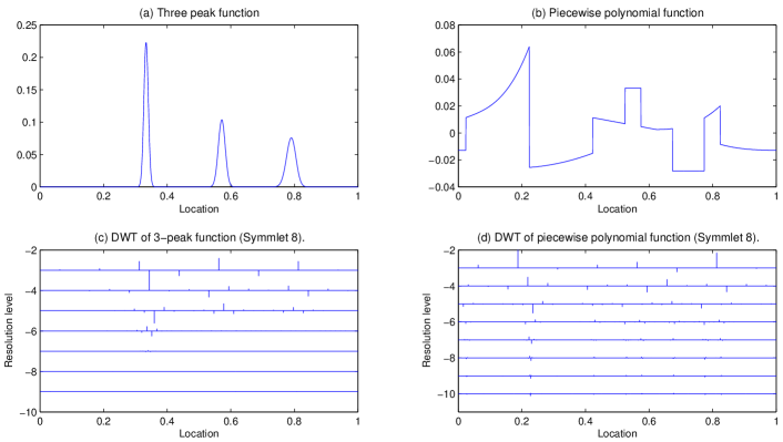
Figure 1: (a) peak: three-peak function evaluated at 1024 equispaced locations; (b) poly: piecewise polynomial function evaluated at 2048 equispaced locations; (c) wc-peak: discrete wavelet transform (DWT) of the three-peak function; (d) wc-poly: DWT of the piecewise polynomial function. In Plot (c) and (d), each vertical bar is proportional in length to the magnitude of the Symmlet 8 wavelet coefficient at the given location and resolution level.

losses	$d_{1}$	FIT-SSVD		LSHM		PMD-SVD		SVD
		median	MAD	median	MAD	median	MAD	median	MAD
$L_{space}(\mathbf{u}_{1},{\hat{\mathbf{u}}}_{1})$	50	0.0513	0.0009	0.0669	0.0014	0.0783	0.0007	0.5225	0.0034
	100	0.0127	0.0003	0.0159	0.0004	0.0254	0.0002	0.1114	0.0005
	200	0.0036	0.0001	0.0044	0.0001	0.0102	0.0000	0.0264	0.0001
$L_{space}(\mathbf{v}_{1},{\hat{\mathbf{v}}}_{1})$	50	0.0958	0.0008	0.1095	0.0016	0.1399	0.0008	0.6330	0.0025
	100	0.0325	0.0004	0.0385	0.0005	0.0566	0.0003	0.1878	0.0006
	200	0.0112	0.0001	0.0131	0.0002	0.0241	0.0001	0.0499	0.0001
$L(\Xi,\hat{\Xi})$	50	0.1454	0.0014	0.1726	0.0019	0.3280	0.0016	2.2217	0.0082
	100	0.0457	0.0004	0.0549	0.0007	0.0973	0.0003	0.3709	0.0009
	200	0.0149	0.0001	0.0177	0.0003	0.0364	0.0001	0.0805	0.0002
$\|{\hat{\mathbf{u}}}_{1}\|_{0}$	50	24	0.1483	22	0.2965	242.5	1.4085	1024	0
	100	34	0.1483	32	0.2965	372.5	1.4085	1024	0
	200	43	0.1483	41	0.2965	577.0	1.3343	1024	0
$\|{\hat{\mathbf{v}}}_{1}\|_{0}$	50	18	0.2965	14	0.2965	535.0	2.2239	2048	0
	100	40	0.2965	38	0.4448	854.5	1.7050	2048	0
	200	66	0.4448	64	0.6672	1303.0	2.0756	2048	0
time	50	0.3364	0.0096	36.7316	0.4497	2.0578	0.0129	1	0
	100	0.4401	0.0209	30.8268	0.3305	1.9607	0.0124	1	0
	200	0.5685	0.0360	23.7639	0.2542	1.9274	0.0102	1	0

Table 1: Comparison of four methods in the rank-one case: $\mathbf{u}_{1}$ is wc-peak, $\mathbf{v}_{1}$ is wc-poly, and the noise is iid N(0,1).

For each simulated scenarios, we ran $100$ simulations, applied each algorithm under comparison, and summarized the results in terms of median and MAD-based standard error. The criteria which we use for comparison of the methods are best explained with reference to Table 1, where we report the results for iid $N(0,1)$ noise $Z$:

• The first block examines the estimation accuracy of the left singular vector, with the three rows corresponding to three different values of $d_{1}$. Following Ma (2011), we define the loss function for estimating the column space of $U$ for a general rank-$r$ by $L_{space}(U,{\hat{U}})=\|P_{U}-P_{\hat{U}}\|_{2}^{2}$ , where $P_{U}=UU^{\prime}$ is the projection matrix onto the subspace spanned by the columns of $U$ (which is of size $n\times r$ and has orthonormal columns, $U^{\prime}U=I_{r}$). In the rank-one case here, the loss reduces to $\sin^{2}\angle(\mathbf{u}_{1},{\hat{\mathbf{u}}}_{1})$.

• The second block in Table 1 reports the loss for right singular vectors.

• The third block shows the scaled recovery error for the low-rank signal matrix $\Xi=UDV^{\prime}$, defined as $L(\Xi,\hat{\Xi})={\|\hat{\Xi}-\Xi\|_{F}^{2}}/{\|\Xi\|_{F}^{2}}$. Here, $\hat{\Xi}={\hat{U}}{\hat{D}}{\hat{V}}^{\prime}$ and ${\hat{D}}=diag({\hat{d}}_{1},\ldots,{\hat{d}}_{r})$ with diagonal entries being ${\hat{d}}_{l}={\hat{\mathbf{u}}}_{l}^{\prime}X{\hat{\mathbf{v}}}_{l}$.

• The fourth and fifth panels of Table 1 show the sparsity of the solutions measured by $\|{\hat{\mathbf{u}}}_{1}\|_{0}$ and $\|{\hat{\mathbf{v}}}_{1}\|_{0}$, that is, the number of nonzero elements in the estimates.

• The last block shows timing results as a fraction or multiple of the ordinary SVD.

The results are as follows:

• From the first three blocks we see that FIT-SSVD uniformly outperforms the other methods with respect to the three statistical criteria. While LSHM is not far behind FIT-SSVD, PMD-SVD lags in several cases by a factor of two or more. The ordinary SVD fails entirely for low signal strength as the results for $d_{1}=50$ illustrate, impressing the need to leverage sparsity in such situations. Rather expectedly, all methods achieve better statistical accuracy as the signal strength $d_{1}$ increases

• As for the sparsity metrics, FIT-SSVD and LSHM produce similar levels of sparsity, while PMD-SVD estimators are much denser. The results also suggest that as the signal strength $d_{1}$ gets stronger, the three sparse SVD methods estimate more coordinates.

• Finally, the timing results indicate that FIT-SSVD is faster than all other methods, the ordinary SVD included. LSHM stands out as slower than FIT-SSVD by factors of over 40 to over 100. PMD-SVD is more competitive but still at least a factor of three slower than FIT-SSVD. The variation in time for PMD-SVD is small because the majority is spent in cross-validation.

To examine the effect of heavy-tailed noise, we report in Table 2 the simulation results when the entries of the noise matrix $Z$ are distributed iid $\sqrt{3/5}\,t_{5}$, all else being the same as in Table 1. [Recall that the scaling factor $\sqrt{3/5}$ is used to ensure unit variance.] The statistical performance for all methods is worse than in Table 1. In terms of the statistical metrics, the performances of FIT-SSVD and LSHM are in a statistical dead heat, whereas PMD-SVD trails behind by as much as a factor of two in the case of high signal strength, $d_{1}=200$. Again, FIT-SSVD and LSHM have comparable sparsities, whereas PMD-SVD is much denser. In terms of computation time, again FIT-SSVD is uniformly fastest, followed by PMD-SVD which trails by factors of over two to over five, and LSHM being orders of magnitude slower (by factors of 28 to 110).

losses	$d_{1}$	FIT-SSVD		LSHM		PMD-SVD		SVD
		median	MAD	median	MAD	median	MAD	median	MAD
$L_{space}(\mathbf{u}_{1},{\hat{\mathbf{u}}}_{1})$	50	0.0802	0.0015	0.0819	0.0017	0.0907	0.0011	0.5405	0.0037
	100	0.0177	0.0003	0.0180	0.0004	0.0282	0.0003	0.1115	0.0006
	200	0.0048	0.0001	0.0047	0.0001	0.0108	0.0001	0.0262	0.0002
$L_{space}(\mathbf{v}_{1},{\hat{\mathbf{v}}}_{1})$	50	0.1193	0.0014	0.1191	0.0018	0.1560	0.0014	0.6432	0.0039
	100	0.0451	0.0005	0.0415	0.0007	0.0601	0.0003	0.1870	0.0006
	200	0.0145	0.0002	0.0137	0.0002	0.0249	0.0001	0.0498	0.0002
$L(\Xi,\hat{\Xi})$	50	0.1944	0.0024	0.1937	0.0028	0.3719	0.0028	2.2624	0.0107
	100	0.0625	0.0007	0.0600	0.0009	0.1041	0.0005	0.3706	0.0011
	200	0.0192	0.0002	0.0187	0.0002	0.0378	0.0001	0.0805	0.0002
$\|{\hat{\mathbf{u}}}_{1}\|_{0}$	50	20	0.2965	21.5	0.3706	235.0	1.5567	1024	0
	100	31	0.1483	33.0	0.2965	364.0	1.8532	1024	0
	200	40	0.1483	41.0	0.2965	569.5	2.0015	1024	0
$\|{\hat{\mathbf{v}}}_{1}\|_{0}$	50	13	0.1483	14.0	0.2965	526.0	2.0015	2048	0
	100	31	0.2965	38.5	0.5189	841.5	2.1498	2048	0
	200	56	0.2965	64.5	0.6672	1307.5	2.2980	2048	0
time	50	0.3714	0.0190	41.0695	0.9339	2.0826	0.0046	1	0
	100	0.8072	0.0652	30.5216	0.3774	2.0187	0.0039	1	0
	200	0.8238	0.0710	23.0527	0.2554	1.9520	0.0048	1	0

Table 2: Comparison of four methods in the rank-one case: $\mathbf{u}_{1}$ is wc-peak, $\mathbf{v}_{1}$ is wc-poly, and the noise is iid ${\scriptstyle\sqrt{3/5}}\,t_{5}$.

3.2 Rank-two results

We show next simulation results for data according to model (1) with $r=2$, and again $n=1024$ and $p=2048$. The singular values $(d_{1},d_{2})$ range among the pairs $(100,50)$, $(200,50)$, and $(200,100)$. The singular vectors are $\mathbf{u}_{1}=$ wc-peak, $\mathbf{v}_{1}=$wc-poly, $\mathbf{u}_{2}=$ wc-step, and $\mathbf{v}_{2}=$ wc-sing, the properties of the latter two vectors being shown in Figure 2.

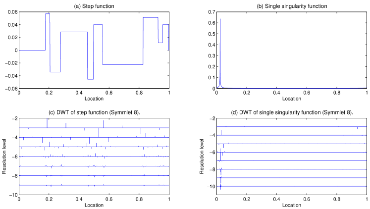
Figure 2: (a)step: step function evaluated at 1024 equispaced locations, (b)sing: single singularity function evaluated at 2048 equispaced locations, (c)wc-step: DWT of step function, (d)wc-sing: DWT of single singularity function.

Table 3 reports the results from $100$ repetitions when the noise is iid $N(0,1)$. In terms of statistical metrics, FIT-SSVD always outperforms LSHM though not hugely. PMD-SVD does slightly better than FIT-SSVD for $L_{space}(U,{\hat{U}})$, but much worse for $L_{space}(V,{\hat{V}})$ and $L(\Xi,\hat{\Xi})$. This is due to the special type of cross-validation used in the package PMA: the parameters $s_{u},s_{v}$ are set to be proportional to each other after being scaled according to the dimensionality, $\sqrt{n}$ and $\sqrt{p}$, which essentially reduces the simultaneous cross-validation on two parameters to one. Therefore, PMD-SVD actually enforces the same level of sparsity on ${\hat{\mathbf{u}}}$ and ${\hat{\mathbf{v}}}$.

In terms of sparsity of the estimators, the fourth and fifth blocks show the cardinality of the joint support of the estimated singular vectors, which indicate that FIT-SSVD and LSHM are again about comparable, and PMD-SVD is much denser as in the rank-one case. [We do not compare the losses and the $l_{0}$ norms for individual singular vectors because LSHM and PMD-SVD do not produce orthogonal singular vectors.]

Finally, in terms of computation time, FIT-SSVD dominates again, and the differences become somewhat more pronounced than in the rank-one case. In the high signal scenario, $d_{1}=200$ and $d_{2}=100$, FIT-SSVD gets a boost because by avoiding the costly bootstrap in Algorithm 3 because Condition 3 is satisfied and the much cheaper normal approximation on Line 3 of Algorithm 3 can be used to compute the threshold level. Since LSHM repeats its scheme on the residual matrix to get the second layer of SVD, computation time doubles. As for PMD-SVD, since the time is mainly spent in cross-validation and the same penalty parameter is used for different ranks, the increase in time is not obvious.

losses	$d_{1}$	$d_{2}$	FIT-SSVD		LSHM		PMD-SVD		SVD
			median	MAD	median	MAD	median	MAD	median	MAD
$L_{space}(U,{\hat{U}})$	100	50	0.1163	0.0010	0.1413	0.0021	0.1022	0.0009	0.5315	0.0037
	200	50	0.1148	0.0013	0.1422	0.0018	0.1007	0.0009	0.5265	0.0027
	200	100	0.0376	0.0003	0.0443	0.0006	0.0321	0.0003	0.1114	0.0005
$L_{space}(V,{\hat{V}})$	100	50	0.0514	0.0009	0.0596	0.0010	0.1230	0.0008	0.6376	0.0029
	200	50	0.0506	0.0009	0.0601	0.0011	0.1259	0.0006	0.6293	0.0023
	200	100	0.0144	0.0002	0.0172	0.0003	0.0538	0.0002	0.1870	0.0005
$L(\Xi,\hat{\Xi})$	100	50	0.0691	0.0006	0.0825	0.0007	0.1403	0.0004	0.7439	0.0017
	200	50	0.0234	0.0001	0.0285	0.0002	0.0529	0.0001	0.2070	0.0005
	200	100	0.0228	0.0001	0.0261	0.0002	0.0483	0.0001	0.1387	0.0003
$|supp({\hat{\mathbf{u}}}_{1})\cup supp({\hat{\mathbf{u}}}_{2})|$	100	50	49	0.2965	45.0	0.4448	479	1.1861	1024	0
	200	50	56	0.2965	49.0	0.2965	649	1.5567	1024	0
	200	100	77	0.2965	73.5	0.5189	657	1.3343	1024	0
$|supp({\hat{\mathbf{v}}}_{1})\cup supp({\hat{\mathbf{v}}}_{2})|$	100	50	54	0.2965	50.5	0.3706	1158.0	2.2239	2048	0
	200	50	78	0.2965	74.5	0.5189	1486.5	2.1498	2048	0
	200	100	81	0.4448	82.5	0.5930	1623.0	2.1498	2048	0
time	100	50	1.1675	0.0829	64.7840	0.6037	2.7991	0.0141	1	0
	200	50	1.4572	0.1011	55.6839	0.5436	2.7018	0.0142	1	0
	200	100	0.8000	0.0668	54.2361	0.2363	2.6429	0.0073	1	0

Table 3: Comparison of four methods for the rank-two case, with noise iid $N(0,1)$.

4 Real data examples

All the methods mentioned above require sparse singular vectors (with most entries close to zero). One source of such data is two-way functional data whose row and column domains are both structured, for example, temporally or spatially, as when the data are time series collected at different locations in space. Two-way functional data are usually smooth as functions of the row and column domains. Thus, if we expand them in suitable basis functions, such as an orthonormal trigonometric basis, the coefficients should be sparse (Johnstone, 2011).

4.1 Mortality rate data

As our first example we use the US mortality rate data from the Berkeley Human Mortality Database (http://www.mortality.org/). They contain mortality rates in the United States for ages 0 to 110 from 1933 to 2007. The data for people older than 95 was discarded because of their noisy nature. The matrix $X$ is of size $96\times 75$, each row corresponding to an age group and each column to a one-year period. We first pre- and post- multiply the data matrix with orthogonal matrices whose columns are the eigenvectors of second order difference matrices of proper sizes; the result is a matrix of coefficients of the same size as $X$. The rank of the signal is estimated to be 2 using bi-crossvalidation (Section 2.3). We then applied FIT-SSVD, LSHM, PMD-SVD and ordinary SVD to get the first two pairs of singular vectors. Finally, we transformed the sparse estimators of the singular vectors back to the original basis to get smooth singular vectors.

The estimated number of nonzero elements in each singular vector (before the back transformation) is summarized in Table 4: none gives very sparse solutions. This is reasonable, because the mortality rate data is of low noise and for data with no noise we should just use the ordinary SVD. Because this data is of small size, it only takes a few seconds for all the algorithms. The plot of singular vectors for all the methods are shown in Figures 3 to 7. The red dashed line in the left plot is for FIT-SSVD, in the middle for LSHM, and on the right for PMD-SVD. We use the wider gray curve for the ordinary SVD as a reference.

	FIT-SSVD	LSHM	PMD-SVD	SVD
$\|{\hat{\mathbf{u}}}_{1}\|_{0}$	82	48	96	96
$\|{\hat{\mathbf{u}}}_{2}\|_{0}$	86	56	7	96
$\|{\hat{\mathbf{v}}}_{1}\|_{0}$	66	45	75	75
$\|{\hat{\mathbf{v}}}_{2}\|_{0}$	70	45	43	75

Table 4: Mortality data: number of nonzero coordinates in the transformed domain for four methods.

Figure 3 shows the first left singular vector plotted against age. The curve ${\hat{\mathbf{u}}}_{1}$ shows a pattern for mortality as a function of age: a sharp drop between age 0 and 2, then a gradual decrease till the teen years, flat till the 30s, after which begins an exponential increase. Figure 4 zooms into the lower left corner of Figure 3 to show the details between age 0 and 10. LSHM, as always turns out to be the sparsest (or smoothest) among the three iterative procedures in the transformed (or original) domain. We believe that FIT-SSVD and PMD-SVD make more sense based on a parallel coordinates plot of the raw data (not shown here), in which the drop in the early age appears to be sharp and therefore should not be smoothed out. Figure 5 shows the first right singular vectors plotted against year. It implies that mortality decreases with time. All of the panels show a wiggly structure, with LSHM again being the smoothest. Here, too, we believe that the zigzag structure is real and not due to noise in the raw data, based again on a parallel coordinate plot of the raw data. The zigzags may well be systematic artifacts, but they are unlikely to be noise.

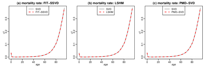
Figure 3: Mortality data: plot of ${\hat{\mathbf{u}}}_{1}$. Panel (a): FIT-SSVD vs. SVD; Panel (b): LSHM vs. SVD; Panel (c): PMD-SVD vs. SVD.

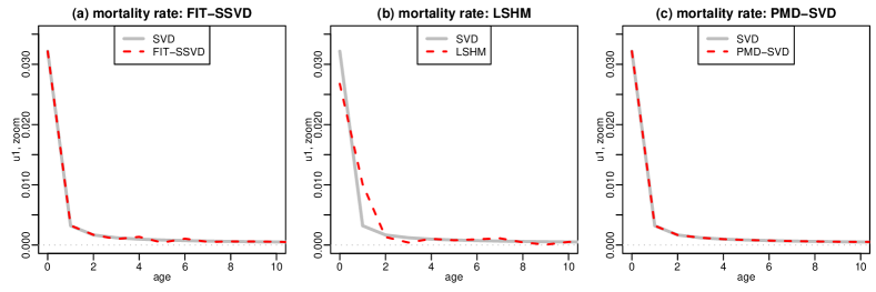
Figure 4: Mortality data: Plot of ${\hat{\mathbf{u}}}_{1}$. Zoom of the lower left corner of Figure 3. Everything else is the same as in Figure 3.

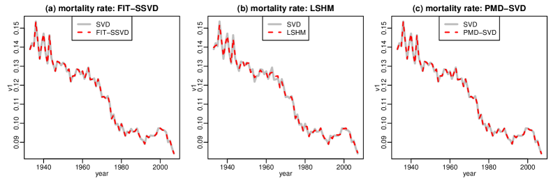
Figure 5: Mortality data: Plot of ${\hat{\mathbf{v}}}_{1}$. Everything else is the same as in Figure 3.

The second pair of singular vectors is shown in Figures 6 and 7: They correct the pattern that the first pair of singular vectors does not capture. The contrast mainly focuses on people younger than 2 or between 60 and 90 where ${\hat{\mathbf{u}}}_{2}$ is positive. Also, ${\hat{\mathbf{v}}}_{2}$ has extreme negative or positive values towards the both ends, 1940s and 2000s. Together, they suggest that babies and older people had lower mortality rates in the 1940s and higher mortality rates in the 2000s than what the first component expresses. One final aspect to note is the strange behavior of ${\hat{\mathbf{u}}}_{2,PMD-SVD}$, recalling that ${\hat{\mathbf{u}}}_{1,PMD-SVD},{\hat{\mathbf{v}}}_{1,PMD-SVD},{\hat{\mathbf{v}}}_{2,PMD-SVD}$ all follow the ordinary SVD very closely. We think this is again due to the cross-validation technique they use.

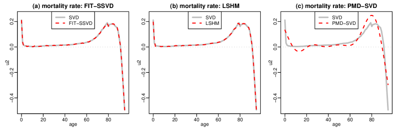
Figure 6: Mortality data: plot of ${\hat{\mathbf{u}}}_{2}$. Everything else is the same as Figure 3.

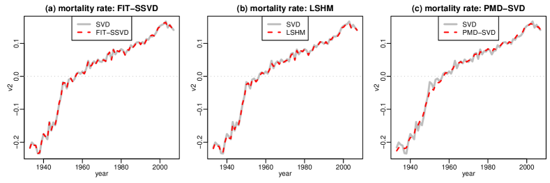
Figure 7: Mortality data: plot of ${\hat{\mathbf{v}}}_{2}$. Everything else is the same as Figure 3.

Huang et al. (2009) also used the mortality data from 1959 to 1999 to illustrate their version of regularized SVDs to get smooth singular vectors by adding second order difference penalties. If we compare the results shown in this section with theirs, our solutions lack the smoothness of their solutions, but we think we recover more information from the data by capturing not only the general trend but also local details such as year-to-year fluctuations.

4.2 Cancer data

We consider next another data example where some sparse structure may be expected to exist naturally. The cancer data used by Lee et al. (2010a) (who in turn have them from Liu et al. (2008)) consists of the gene expression levels of 12,625 genes for 56 cases of four different types of cancer. It is believed that only a part of the genes regulate the types and hence the singular vectors corresponding to the genes should ideally be sparse. We apply the four SVD methods directly to the raw data without change of basis.

Before we proceed it may be proper to discuss briefly some modeling ambiguities posed by this dataset as it is not a priori clear whether a PCA or SVD model is more appropriate. It might be argued that the cases really should be considered as being sampled from a population, hence PCA would be the proper analysis, with the genes representing the variables. The counter argument is, however, that the cases are stratified, and the strata are pure convenience samples of sizes that bear no relation to the sizes of naturally occurring cancer populations. A dual interpretation with genes as samples and cases as variables would be conceivable also, but it seems even more far fetched in the absence of any sampling aspect with regard to genes. In light of the problems raised by any sampling assumption, it would seem more appropriate to condition on the cases and the genes and adopt a fixed effects view of the data. As a result the SVD model seems less problematic than either of the dual PCA models.

We first attempted to estimate the rank of the signal using bi-crossvalidation (Section 2.3), but it turns out that the rank is sensitive to the choice of $\alpha$ (Holm family-wise error) and $\beta$ (Huberization quantile) in Algorithm 2, ranging from $r$=3 to $r$=5. We decided to use $r=3$ because this is the number of contrasts required to cluster the cases into four groups. Also, this is the rank used by Lee et al. (2010a), which grants comparison of their and our results.

On a different note, running LSHM on these data with rank three took a couple of hours, which may be a disincentive for users to seek even higher ranks. The hours of run time of LSHM compares with a few minutes for PMD-SVD and merely a few seconds for FIT-SSVD. (In addition, LSHM’s third singular vectors do not seem to converge within 300 iterations.)

Table 5 summarizes the cardinalities of the union of supports of three singular vectors for each method. For the estimation of left singular vectors corresponding to different genes, the PMD-SVD solution is undesirably dense, while FIT-SSVD and LSHM give similar levels of sparsity. For the estimation of right singular vectors corresponding to the cases, we would expect that all cases have their own effects rather than zero, so it is not surprising that the estimated singular vectors are dense.

	FIT-SSVD	LSHM	PMD-SVD	SVD
$|\cup_{l=1}^{3}\mathrm{supp}({\hat{\mathbf{u}}}_{l})|$	4688	4545	12625	12625
$|\cup_{l=1}^{3}\mathrm{supp}({\hat{\mathbf{v}}}_{l})|$	56	56	54	56

Table 5: Cancer data: summary of cardinality of joint support of three singular vectors for four methods.

Figure 8 shows the scatterplots of the entries of the first three right singular vectors for the four methods. Points represent patients, each row represents one method, and each column corresponds to two of the three singular vectors. The four known groups of patients are easily discerned in the plots. A curiosity is the cross-wise structure produced by PMD-SVD, where the singular vectors are nearly mutually exclusive: if one coordinate in a singular vector is non-zero, most corresponding coordinates in the other singular vectors are zero. The other three methods, including the ordinary SVD, agree strongly among each other in the placement of the patients. The agreement with the ordinary SVD is not a surprise as $p=56$ is a relatively small column dimension on which sparsity may play a less critical role compared to the row dimension with $n=12625$. Yet, the three sparse methods give clearer evidence that the carcinoid group (black cirlces) falls into two subgroups than the ordinary SVD. According to FIT-SSVD and LSHM the separation is along ${\hat{\mathbf{v}}}_{3}$ (center and right hand plots), whereas according to PMD-SVD it is by lineup with ${\hat{\mathbf{v}}}1$ and ${\hat{\mathbf{v}}}2$, respectively (left hand plot).

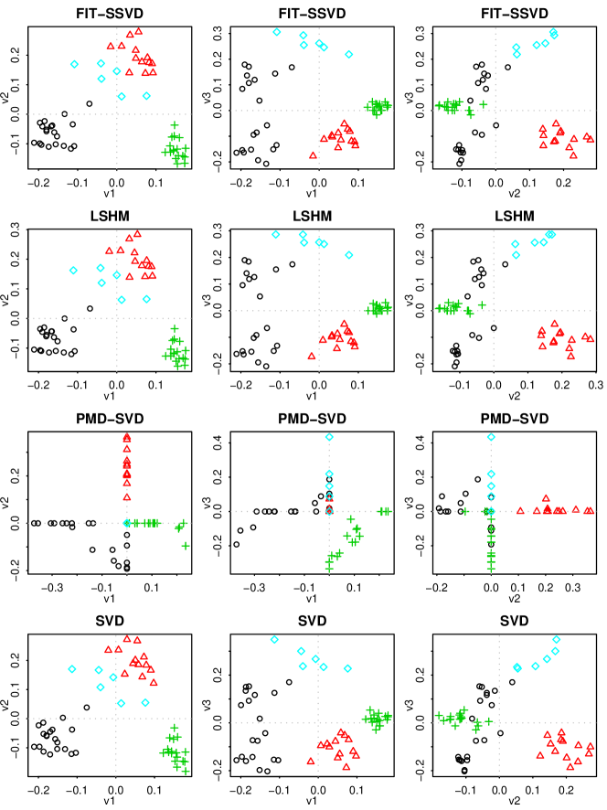
Figure 8: Cancer data: Scatterplots of the entries of the first three right singular vectors ${\hat{\mathbf{v}}}_{l},l=1,2,3$ for four methods. Points represent patients. Black circle: Carcinoid; Red triangle: Colon; Green cross: Normal; Blue diamond: SmallCell.

Figure 9 shows checkerboard plots of the reconstructed rank-three approximations, layed out with patients on the vertical axis and genes on the horizontal axis. Each row of plots represents one method, and the plots in a given row show the same reconstructed matrix but successively ordered according to the coordinates of the estimated left singular vectors ${\hat{\mathbf{u}}}_{1}$, ${\hat{\mathbf{u}}}_{2}$ and ${\hat{\mathbf{u}}}_{3}$. There are fewer than 5000 genes shown for FIT-SSVD and LSHM, because the rest are estimated to be zero, whereas all 12,625 genes are shown for PMD-SVD and SVD (Table 5). We can see clear checkerboard structure in some of the plots, indicating biclustering. In spite of the strong similarity between the patient projections for FIT-SSVD and LSHM in Figure 8, there is a clear difference between these methods in the reconstructions in Figure 9: The FIT-SSVD solution exhibits the strongest block structure in its ${\hat{\mathbf{u}}}_{2}$-based sort (center plot, top row), implying the strongest evidence of clustering among its non-thresholded genes. Since these blocks consist of many hundreds of genes, it would surprisingly suggest that the differences between the four patient groups run into the hundreds, not dozens, of genes.

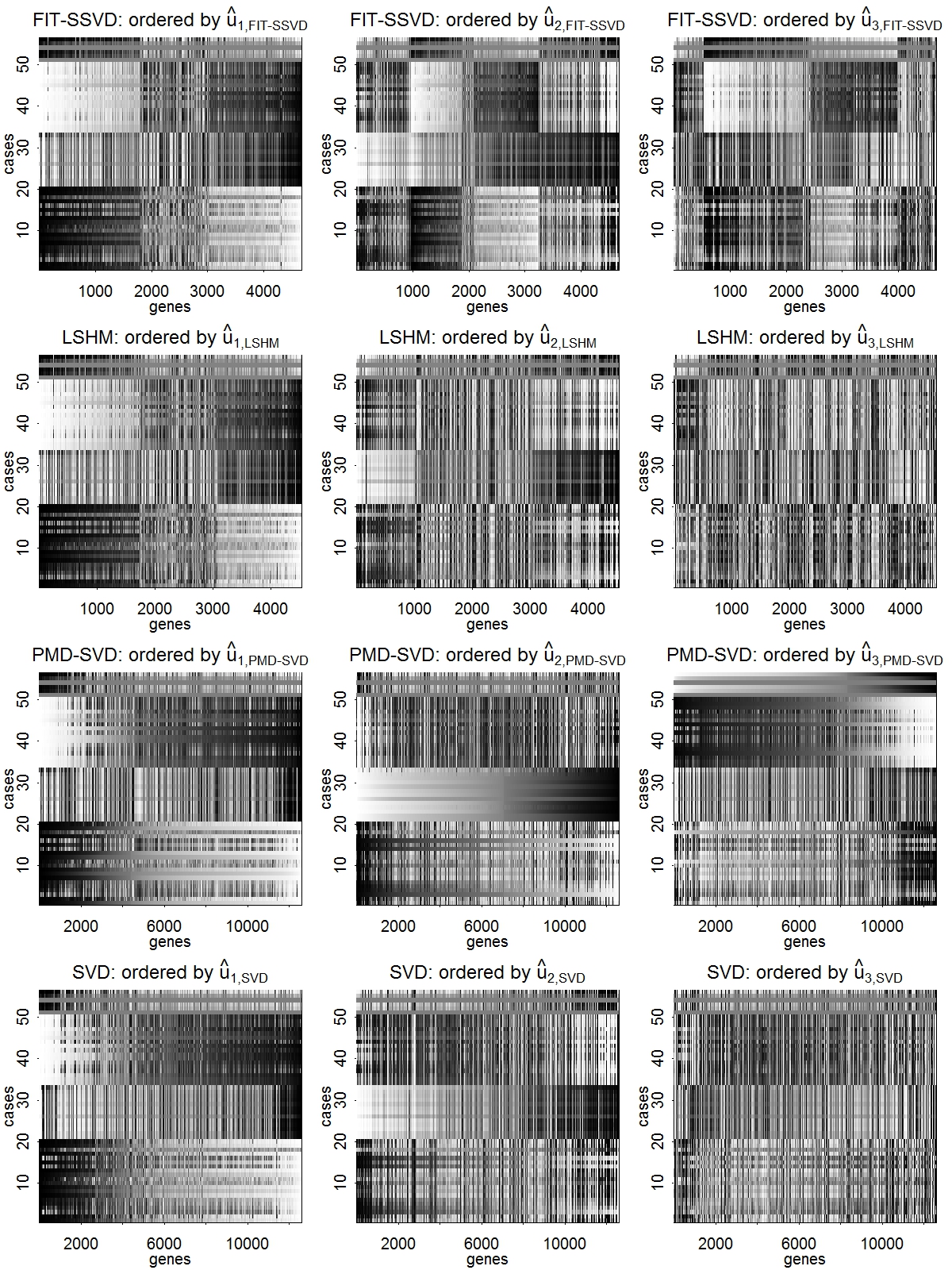
Figure 9: Cancer data: Image plots of the rank-three approximations $\sum_{l=1,2,3}{\hat{d}}_{l}{\hat{\mathbf{u}}}_{l}{\hat{\mathbf{v}}}_{l}^{\prime}$ whose values are gray-coded. Each image is laid out as cases (= rows) by genes (= columns). The same rank-three approximation is shown three times for each method (left to right), each time sorted according to a different ${\hat{\mathbf{u}}}_{l}$ ($l=1,2,3$). (The mapping of the rank-three approximation values to gray scales is by way of a rank transformation, using a separate transformation for each image. Rank transformations create essentially uniform distributions that better cover the range of gray scale values.)

In spite of the differences in checkerboard patterns in Figure 9, the three left singular vectors are highly correlated between FIT-SSVD and LSHM: $\mathrm{corr}$ = 0.985, 0.981, and 0.968, respectively, and the top 20 genes with largest magnitude in the estimated three left singular vectors of FIT-SSVD overlap with those of LSHM except for one gene in the second singular vector. These shared performance aspects notwithstanding, the two methods differ hugely in computing time, FIT-SSVD taking seconds, LSHM taking a couple of hours.

5 Discussion

We presented a procedure, called FIT-SSVD, for the fast and simultaneous extraction of singular vectors that are sparse in both the row and the column dimension. While the procedure is state of the art in terms of statistical performance, its overriding advantage is sheer speed. The reasons why speed matters are several: (1) Faster algorithms enable the processing of larger datasets. (2) The use of SVDs in data analysis is most often for exploratory ends which call for unlimited iterations of quickly improvised steps — something that is harder to achieve as datasets grow larger. (3) Sparse multivariate technology is still a novelty and hence at an experimental stage; if its implementation is fast, early adopters of the technology have a better chance to rapidly gain experience by experimenting with its parameters. (4) If a statistical method such as sparse SVD has a fast implementation, it can be incorporated as a building block in larger methodologies, for example, in processing data arrays that are more than two-dimensional. For these reasons we believe that fast SVD technology is of the essence for its success.

A unique opportunity for sparse approaches is to achieve faster speed than standard non-sparse approaches when the structure in the data is truly sparse. Our algorithm achieves this to some extent through initialization that is both sparse and smart: sparse initialization consists of a standard SVD of smaller size than the full data matrix, while smart (in particular: non-random) initialization reduces the number of iterations to convergence. A statistical benefit is that inconsistent estimation by the standard SVD on large data matrices with weak signal is avoided. — An imperative for fast implementations is avoiding where possible such slow devices as cross-validation. A considerable speed advantage we achieve is through relatively fast (non-crossvalidated) selection of thresholding levels based on an analytical understanding of their function.

Our proposal has conceptual and theoretical features that are unique at this stage of the development of the field: (1) FIT-SSVD extracts $r$ orthogonal left- and right-singular vectors simultaneously, which puts it more in line with standard linear dimension reduction where orthogonal data projections are the norm. In addition, simultaneous extraction can be cast as subspace extraction, which provides a degree of immunity to non-identifiability and slow convergence of individual singular vectors when some of the first $r$ underlying singular values are nearly tied: since we measure convergence in terms of distance between successive $r$-dimensional subspaces, our algorithm does not need to waste effort in pinning down ill-determined singular vectors as long as the left- and right-singular subspaces are well-determined. Such a holistic view of the rank-$r$ approximation is only available to simultaneous but not to successive extraction. (2) FIT-SSVD is derived from asymptotic theory that preceded its realization as a methodology: For Gaussian noise in the model (1), we (Yang et al., 2011) showed that our algorithm with appropriately chosen parameters achieves the rate of the minimax lower bound. In other words, in a specific parameter space, our algorithm is asymptotically optimal in terms of minimizing the maximum possible risk over the whole parameter space.

As for future work, the current state of the art raises several questions. For one, it would be of interest to better understand the relative merits of the currently proposed sparse SVD approaches since they have essential features in common, such as power iterations and thresholding. Another natural question arises from the fact that sparse SVDs build on the sequence model: many methods for choosing parameters from the data have been shown to be asymptotically equivalent to first order in the sequence model (see, e.g., Haerdle et al. (1988)), including cross-validation, generalized cross-validation, Rice’s method based on unbiased estimates of risk, final prediction error, and the Akaike information criterion. Do these asymptotic equivalences hold in the matrix setting for sparse SVD approaches? How does the choice of the BIC in LSHM compare? Also, our algorithm and underlying theory allow a wide range of thresholding functions: Is there an optimal choice in some sense? Further, there exists still a partial disconnect between asymptotic theory and practical methodology: The theory requires a strict rank $r$ model, whereas by all empirical evidence the algorithm works well in a “trailing rank” situation where real but small singular values exist. Finally, there is a robustness aspect that is specific to sparse SVD approaches: heavier than normal tails in the noise distribution generate “random factors” caused by single outlying cells. While we think we have made reasonable and empirically successful choices in drawing from the toolkit of robustness, we have not provided a theoretical framework to justify them. — Just the same, even if the proposed FIT-SSVD algorithm may be subject to some future tweaking, in the substance it has the promise of lasting merit.

References

- Allen et al. (2011) G. I. Allen, L. Grosenick, and J. Taylor. A generalized least squares matrix decomposition. Rice University Technical Report No. TR2011-03, 2011.
- Alter et al. (2001) O. Alter, P. O. Brown, and D. Botstein. Processing and modeling genome-wide expression data using singular value decomposition. Proc. Natl. Acad. Sci., 97(18):10101–10106, 2001.
- Bach et al. (2008) F. Bach, J. Mairal, and J. Ponce. Convex sparse matrix factorizations. CoRR, abs/0812.1869, 2008.
- Bickel et al. (1997) P. J. Bickel, F. Gotze, and W. R. Van Zwet. Resampling fewer than n observations: gains, losses, and remedies for losses. Statist. Sinica, 7:1–32, 1997.
- Fan and Li (2001) J. Fan and R. Li. Variable selection via nonconcave penalized likelihood and its oracle properties. J. Am. Stat. Assoc., 96:1348–1360, 2001.
- Gabriel (2002) K. R. Gabriel. Journal de la Societe Francaise de Statistique, 143(3):5–56, 2002.
- Golub and Van Loan (1996) G. H. Golub and C. F. Van Loan. Matrix computations (3rd ed.). Johns Hopkins University Press, 1996. ISBN 0801854148.
- Hoff (2007) P. D. Hoff. Model averaging and dimension selection for the singular value decomposition. J. Am. Stat. Assoc., 102(478):674–685, 2007.
- Holm (1979) S. Holm. A simple sequentially rejective multiple test procedure. Scand. J. Statist., 6:65–70, 1979.
- Huang et al. (2009) J. Z. Huang, H. Shen, and A. Buja. The analysis of two-way functional data using two-way regularized singular value decompositions. J. Am. Stat. Assoc., 104(488):1609–1620, 2009.
- Johnstone (2011) I. M. Johnstone. Gaussian estimation: Sequence and multiresolution models. Available at http://www-stat.stanford.edu/~imj/, 2011.
- Johnstone and Lu (2009) I. M. Johnstone and A. Y. Lu. On consistency and sparsity for principal components analysis in high dimensions. J. Am. Stat. Assoc., 104(486):682–693, 2009.
- Lee et al. (2010a) M. Lee, H. Shen, J. Z. Huang, and J. S. Marron. Biclustering via sparse singular value decomposition. Biometrics, 66:1087–1095, 2010a.
- Lee et al. (2010b) M. Lee, H. Shen, J. Z. Huang, and J. S. Marron. R code for LSHM, 2010b. URL http://www.unc.edu/~haipeng/publication/ssvd-code.rar.
- Liu et al. (2008) Y. Liu, D. N. N. Hayes, A. Nobel, and J. S. Marron. Statistical significance of clustering for High-Dimension, Low-Sample size data. J. Am. Stat. Assoc., 103(483):1281–1293, 2008.
- Lu (2002) A. Y. Lu. Sparse principal component analysis for functional data. PhD thesis, Stanford University, Stanford, CA, 2002.
- Ma (2011) Z. Ma. Sparse principal component analysis and iterative thresholding. 2011.
- Mairal et al. (2010) J. Mairal, F. Bach, J. Ponce, and G. Sapiro. Online Learning for Matrix Factorization and Sparse Coding. J. Mach. Learn. Res., 11(1):19–60, 2010.
- Mallat (2009) S. Mallat. A Wavelet Tour of Signal Processing: The Sparse Way. Academic Press, 2009.
- Nadler (2009) B. Nadler. Discussion of “On consistency and sparsity for principal components analysis in high dimensions” by Johnstone and Lu. J. Am. Stat. Assoc., 104(486):694–697, 2009.
- Owen and Perry (2009) A. B. Owen and P. O. Perry. Bi-cross-validation of the SVD and the nonnegative matrix factorization. Ann. Appl. Stat., 3:564–594, 2009.
- Paul (2007) D. Paul. Asymptotics of sample eigenstruture for a large dimensional spiked covariance model. Stat. Sinica, 17(4):1617–1642, 2007.
- Paul and Johnstone (2007) D. Paul and I. M. Johnstone. Augmented sparse principal component analysis for high dimensional data. Preprint, available at http://anson.ucdavis.edu/~debashis/techrep/augmented-spca.pdf, 2007.
- Prasantha et al. (2007) H. S. Prasantha, H. L. Shashidhara, and K. N. Balasubramanya Murthy. Image compression using SVD. In Proceedings of the International Conference on Computational Intelligence and Multimedia Applications, pages 143–145. IEEE Computer Society, 2007.
- Shabalin and Nobel (2010) A. Shabalin and A. Nobel. Reconstruction of a low-rank matrix in the presence of gaussian noise. Preprint, availabel at http://arxiv.org/abs/1007.4148, 2010.
- Shen et al. (2011) D. Shen, H. Shen, and J. S. Marron. Consistency of sparse PCA in high dimension, low sample size contexts. 2011.
- Shen and Huang (2008) H. Shen and J. H. Huang. Sparse principal component analysis via regularized low rank matrix approximation. J. Multivariate Anal., 99:1015–1034, 2008.
- Sill et al. (2011) M. Sill, S. Kaiser, A. Benner, and A. Kopp-Schneider. Robust biclustering by sparse singular value decomposition incorporating stability selection. Bioinformatics, 27(15):2089–2097, 2011.
- Thomasian et al. (1998) A. Thomasian, V. Castelli, and C. Li. Clustering and singular value decomposition for approximate indexing in high dimensional spaces. In Proceedings of the seventh international conference on Information and knowledge management, pages 201–207, 1998.
- Witten et al. (2010) D. Witten, R. Tibshirani, and S. Gross. PMA: Penalized Multivariate Analysis, 2010. URL http://CRAN.R-project.org/package=PMA. R package version 1.0.7.
- Witten and Tibshirani (2010) D. M. Witten and R. Tibshirani. A framework for feature selection in clustering. J. Am. Stat. Assoc., 105(490):713–726, 2010.
- Witten et al. (2009) D. M. Witten, R. Tibshirani, and T. Hastie. A penalized matrix decomposition, with applications to sparse principal components and canonical correlation analysis. Biostatistics, 10:515–534, 2009.
- Wold (1978) S. Wold. Cross-validatory estimation of the number of components in factor and principal component models. Technometrics, 20(4):397–405, 1978.
- Yang et al. (2011) D. Yang, Z. Ma, and A. Buja. Near optimal sparse SVD in high dimensions. 2011.
- Zheng et al. (2007) W. Zheng, S. Z. Li, J. H. Lai, and S. Liao. On constrained sparse matrix factorization. Computer Vision, IEEE International Conference on, 0:1–8, 2007.
- Zou et al. (2006) H. Zou, T. Hastie, and R. Tibshirani. Sparse principal component analysis. J. Comput. Graph. Stat., 15:265–286, 2006.