On a Hidden Symmetry of Quantum Harmonic Oscillators

Abstract.

We consider a six-parameter family of the square integrable wave functions for the simple harmonic oscillator, which cannot be obtained by the standard separation of variables. They are given by the action of the corresponding maximal kinematical invariance group on the standard solutions. In addition, the phase space oscillations of the electron position and linear momentum probability distributions are computer animated and some possible applications are briefly discussed. A visualization of the Heisenberg Uncertainty Principle is presented.

The purpose of this Letter is to elaborate on a “missing” class of solutions to the time-dependent Schrödinger equation for the simple harmonic oscillator in one dimension. We also provide an interesting computer-animated feature of these solutions — the phase space oscillations of the electron density and the corresponding probability distribution of the particle linear momentum. As a result, a dynamic visualization of the fundamental Heisenberg Uncertainty Principle [27] is given [45], [62].

1. Symmetry and Hidden Solutions

The time-dependent Schrödinger equation for the simple harmonic oscillator,

$$2i\psi_{t}+\psi_{xx}-x^{2}\psi=0,$$ (1.1)

has the following six-parameter family of square integrable solutions

$$\psi_{n}\left(x,t\right)=\frac{e^{i\left(\alpha\left(t\right)x^{2}+\delta\left(t\right)x+\kappa\left(t\right)\right)+i\left(2n+1\right)\gamma\left(t\right)}}{\sqrt{2^{n}n!\mu\left(t\right)\sqrt{\pi}}}\ e^{-\left(\beta\left(t\right)x+\varepsilon\left(t\right)\right)^{2}/2}\ H_{n}\left(\beta\left(t\right)x+\varepsilon\left(t\right)\right),$$ (1.2)

where $H_{n}\left(x\right)$ are the Hermite polynomials [51] and

$$\mu\left(t\right) = \mu_{0}\sqrt{\beta_{0}^{4}\sin^{2}t+\left(2\alpha_{0}\sin t+\cos t\right)^{2}},$$ (1.3)

$$\alpha\left(t\right) = \frac{\alpha_{0}\cos 2t+\sin 2t\ \left(\beta_{0}^{4}+4\alpha_{0}^{2}-1\right)/4}{\beta_{0}^{4}\sin^{2}t+\left(2\alpha_{0}\sin t+\cos t\right)^{2}},$$ (1.4)

$$\beta\left(t\right) = \frac{\beta_{0}}{\sqrt{\beta_{0}^{4}\sin^{2}t+\left(2\alpha_{0}\sin t+\cos t\right)^{2}}},$$ (1.5)

$$\gamma\left(t\right) = \gamma_{0}-\frac{1}{2}\arctan\frac{\beta_{0}^{2}\sin t}{2\alpha_{0}\sin t+\cos t},$$ (1.6)

$$\delta\left(t\right) = \frac{\delta_{0}\left(2\alpha_{0}\sin t+\cos t\right)+\varepsilon_{0}\beta_{0}^{3}\sin t}{\beta_{0}^{4}\sin^{2}t+\left(2\alpha_{0}\sin t+\cos t\right)^{2}},$$ (1.7)

$$\varepsilon\left(t\right) = \frac{\varepsilon_{0}\left(2\alpha_{0}\sin t+\cos t\right)-\beta_{0}\delta_{0}\sin t}{\sqrt{\beta_{0}^{4}\sin^{2}t+\left(2\alpha_{0}\sin t+\cos t\right)^{2}}},$$ (1.8)

$$\kappa\left(t\right) = \kappa_{0}+\sin^{2}t\ \frac{\varepsilon_{0}\beta_{0}^{2}\left(\alpha_{0}\varepsilon_{0}-\beta_{0}\delta_{0}\right)-\alpha_{0}\delta_{0}^{2}}{\beta_{0}^{4}\sin^{2}t+\left(2\alpha_{0}\sin t+\cos t\right)^{2}}$$

$$+\frac{1}{4}\sin 2t\ \frac{\varepsilon_{0}^{2}\beta_{0}^{2}-\delta_{0}^{2}}{\beta_{0}^{4}\sin^{2}t+\left(2\alpha_{0}\sin t+\cos t\right)^{2}}.$$

(Here, $\mu_{0}>0,$ $\alpha_{0},$ $\beta_{0}\neq 0,$ $\gamma_{0},$ $\delta_{0},$ $\varepsilon_{0},$ $\kappa_{0}$ are real initial data.) These “missing” solutions can be derived analytically in a unified approach to generalized harmonic oscillators (see, for example, [9], [10], [39] and the references therein). They are also verified by a direct substitution with the aid of Mathematica computer algebra system [33], [45], [62]. (The simplest special case $\mu_{0}=\beta_{0}=1$ and $\alpha_{0}=\gamma_{0}=\delta_{0}=\varepsilon_{0}=\kappa_{0}=0$ reproduces the textbook solution obtained by the separation of variables [21], [23], [38], [47]; see also the original Schrödinger paper [55]; and the shape-preserving oscillator evolutions occur when $\alpha_{0}=0$ and $\beta_{0}=1.$ More details on the derivation of these formulas can be found in Refs. [44] and [50]; see also the references therein.)

On the other hand, the “dynamic harmonic oscillator states” (1.2)–(1) are eigenfunctions,

$$E\left(t\right)\psi_{n}\left(x,t\right)=\left(n+\frac{1}{2}\right)\psi_{n}\left(x,t\right),$$ (1.10)

of the time-dependent quadratic invariant,

$$E\left(t\right) = \frac{1}{2}\left[\frac{\left(p-2\alpha x-\delta\right)^{2}}{\beta^{2}}+\left(\beta x+\varepsilon\right)^{2}\right]$$

$$= \frac{1}{2}\left[\widehat{a}\left(t\right)\widehat{a}^{\dagger}\left(t\right)+\widehat{a}^{\dagger}\left(t\right)\widehat{a}\left(t\right)\right],\qquad\frac{d}{dt}\langle E\rangle=0,$$

with the required operator identity [15], [54]:

$$\frac{\partial E}{\partial t}+i^{-1}\left[E,H\right]=0,\qquad H=\frac{1}{2}\left(p^{2}+x^{2}\right).$$ (1.12)

Here, the time-dependent annihilation $\widehat{a}\left(t\right)$ and creation $\widehat{a}^{\dagger}\left(t\right)$ operators are explicitly given by

$$\widehat{a}\left(t\right)=\frac{1}{\sqrt{2}}\left(\beta x+\varepsilon+i\frac{p-2\alpha x-\delta}{\beta}\right),\qquad\widehat{a}^{\dagger}\left(t\right)=\frac{1}{\sqrt{2}}\left(\beta x+\varepsilon-i\frac{p-2\alpha x-\delta}{\beta}\right)$$ (1.13)

with $p=i^{-1}\partial/\partial x$ in terms of our solutions (1.4)–(1). These operators satisfy the canonical commutation relation,

$$\widehat{a}\left(t\right)\widehat{a}^{\dagger}\left(t\right)-\widehat{a}^{\dagger}\left(t\right)\widehat{a}\left(t\right)=1,$$ (1.14)

and the oscillator-type spectrum (1.10) of the dynamic invariant $E$ can be obtained in a standard way by using the Heisenberg–Weyl algebra of the rasing and lowering operators (a “second quantization” [1], [42], the Fock states):

$$\widehat{a}\left(t\right)\Psi_{n}\left(x,t\right)=\sqrt{n}\ \Psi_{n-1}\left(x,t\right),\quad\widehat{a}^{\dagger}\left(t\right)\Psi_{n}\left(x,t\right)=\sqrt{n+1}\ \Psi_{n+1}\left(x,t\right).$$ (1.15)

Here,

$$\psi_{n}\left(x,t\right)=e^{i\left(2n+1\right)\gamma\left(t\right)}\ \Psi_{n}\left(x,t\right)$$ (1.16)

is the relation to the wave functions (1.2) with $\varphi_{n}\left(t\right)=-\left(2n+1\right)\gamma\left(t\right)$ being the nontrivial Lewis phase [42],  [54].

This quadratic dynamic invariant and the corresponding creation and annihilation operators for the generalized harmonic oscillators have been introduced recently in Ref. [54] (see also [10], [15], [59] and the references therein for important special cases). An application to the electromagnetic-field quantization and a generalization of the coherent states are discussed in Refs. [35] and [40].

The key ingredients, the maximum kinematical invariance groups of the free particle and harmonic oscillator, were introduced in [3], [4], [25], [30], [49] and [50] (see also [7], [31], [48], [53], [57], [58], [63] and the references therein). We establish a (hidden symmetry revealing) connection with certain Ermakov-type system which allows us to bypass a complexity of the traditional Lie algebra approach [44] (see [17], [41] and the references therein regarding the Ermakov equation). (A general procedure of obtaining new solutions by acting on any set of given ones by enveloping algebra of generators of the Heisenberg–Weyl group is described in [15].) In addition, the maximal invariance group of the generalized driven harmonic oscillators is shown to be isomorphic to the Schrödinger group of the free particle and the simple harmonic oscillator [44], [49], [50].

2. Discussion

Quantum systems with quadratic Hamiltonians (see, for example, [2], [5], [6], [10], [14], [15], [18], [20], [26], [46], [64], [65], [66], [68] and the references therein) have attracted substantial attention over the years because of their great importance in many advanced quantum problems. Examples are coherent and squeezed states, uncertainty relations, Berry’s phase, quantization of mechanical systems and Hamiltonian cosmology. More applications include, but are not limited to charged particle traps and motion in uniform magnetic fields, molecular spectroscopy and polyatomic molecules in varying external fields, crystals through which an electron is passing and exciting the oscillator modes, and other mode interactions with external fields. Quadratic Hamiltonians have particular applications in quantum electrodynamics because the electromagnetic field can be represented as a set of generalized driven harmonic oscillators [13], [20].

The maximal kinematical invariance group of the simple harmonic oscillator [50] provides the six-parameter family of solutions, namely (1.2) and (1.3)–(1), for an arbitrary choice of the initial data (of the corresponding Ermakov-type system [17], [39], [41], [44]). These “hidden parameters” usually disappear after evaluation of matrix elements and cannot be observed from the spectrum. How to distinguish between these “new dynamic” and the “standard static” harmonic oscillator states (and which of them is realized in a particular measurement) is thus a fundamental problem.

At the same time, the probability density $\left|\psi\left(x,t\right)\right|^{2}$ of the solution (1.2) is obviously moving with time, somewhat contradicting to the standard textbooks [21], [23], [38], [47], [55], – an elementary Mathematica simulation reveals such space oscillations for the simplest “dynamic oscillator states” [44], [45] (see Appendix A for the Mathematica source code). The same is true for the probability distribution of the particle linear momentum due to the Heisenberg Uncertainty Principle [27]. These effects, quite possibly, can be observed experimentally, say in Bose condensates, if the nonlinearity of the Gross–Pitaevskii equation is turned off by the Feshbach resonance [11], [19], [32], [52], [56], [60]. A more elementary example is an electron moving in a uniform magnetic field. By slowly changing the magnetic field, say, from an initially occupied Landau level with the standard solution [38], [43], one may continuously follow the initial wave function evolution (with the quadratic invariant) until the magnetic field becomes a constant once again (a parametric excitation; see, for example, [9], [15], [37], [46] and the references therein). The terminal state will have, in general, the initial conditions that are required for the “dynamic harmonic states” (1.2)–(1) and the probability density should oscillate on the corresponding Landau level just as our solution predicts. However, it is still not clear how to observe this effect experimentally (but these “dynamic harmonic states” will have a nontrivial Berry’s phase [5], [6], [54], [61], [62]).

One may imagine other possible applications, for example, in molecular spectroscopy [46], theory of crystals, quantum optics [24], [66], and cavity quantum electrodynamics [12], [13], [22], [35], [67]. We believe in a dynamic character of the nature [28]. All of that puts the consideration of this Letter into a much broader mathematical and physical context — This may help better understand some intriguing features of quantum motion. (Our example shows that the separation of variables for the time-dependent Schrödinger equations may not always give us the “whole picture”.)

Acknowledgments. We wish to thank Professor Sir Michael Berry, Professor Andrew Bremner, Professor Carlos Castillo-Chávez, Professor Victor V. Dodonov, Professor Martin Engman, Professor Georgy Th. Guria, Dr. Christoph Koutschan, Dr. Sergey I. Kryuchkov, Professor Elliott Lieb, Dr. Francisco F. López-Ruiz, Professor Alex Mahalov, Professor Vladimir I. Man’ko, Dr. Benjamin R. Morin, Professor Peter Paule, Dr. Andrey M. Puchkov, Priv.-Doz. Dr. Andreas Ruffing, Professor Simon Ruijsenaars, Professor Vladimir M. Shabaev, Professor Erwin Suazo, Dr. Nikolay Tishchenko, Professor Luc Vinet and Professor Doron Zeilberger for support, valuable discussions and encouragement. This paper has been initiated during a short visit of one of the authors (SKS) to The Erwin Schrödinger International Institute for Mathematical Physics and we thank Professor Christian Krattenthaler, Fakultät für Mathematik, Universität Wien, for his hospitality. This research is supported in part by the National Science Foundation–Enhancing the Mathematical Sciences Workforce in the 21st Century (EMSW21), award # 0838705; the Alfred P. Sloan Foundation–Sloan National Pipeline Program in the Mathematical and Statistical Sciences, award # LTR 05/19/09; and the National Security Agency–Mathematical & Theoretical Biology Institute—Research program for Undergraduates; award # H98230-09-1-0104.

Appendix A Mathematica source CODE lines[45]

Example 1

The following animation is for the dynamic ground state $n=0$, using $\alpha_{0}=\gamma_{0}=\varepsilon_{0}=0$,  $\beta_{0}=2/3$, $\delta_{0}=1$:

In[1]:=$\displaystyle\mathrm{Animate}\Bigg{[}\text{Plot}\Bigg{[}\left\{\frac{9\sqrt{2}\ e^{-\frac{72\left(x-\ \text{Sin}\left[\frac{1}{500}\pi(-1+T)\right]\right)^{2}}{97+65\ \text{Cos}\left[\frac{1}{250}\pi(-1+T)\right]}}}{\sqrt{97+65\ \text{Cos}\left[\frac{1}{250}\pi(-1+T)\right]}},\ e^{-\frac{4x^{2}}{9}}\right\},\text{$\{x,-3.5,3.5\}$,\ \text{AxesLabel}\text{\ -$>$}}$

$\{x,(\text{Abs}[\psi]){}^{\wedge}2\}$, $\text{PlotRange}\to\{0,2.3\}$, $\text{Filling}\to\{1\to\text{Bottom}\}$, PlotStyle$\to\{\text{Thick},\text{Blue}\}\Bigg{]},\{T,1001\}\Bigg{]}$

Out[1]=

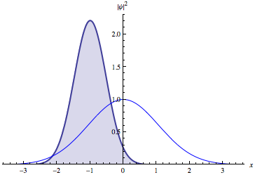
(a)

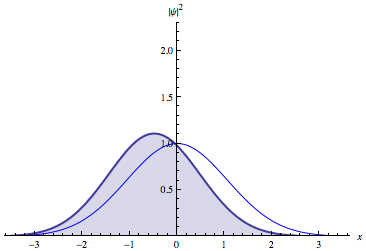
(b)

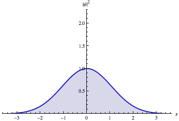
(c)

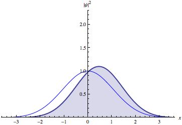
(d)

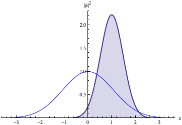
(e)

Figure 1. Subfigures (a)-(e) are a few stills taken from the mathematica movie animation [45]. Starting with (a) they denote the oscillating electron density (blue) of the ground “dynamic harmonic state” of the time-dependent Schrödinger equation (1.1). These space oscillations complement (with the help of Mathematica) the corresponding “static” textbook solution (clear)[55]. (The color version of this figure is available only in the electronic edition.)

Example 2
The following animation is for the first excited dynamic state $n=1$, using $\alpha_{0}=\gamma_{0}=\varepsilon_{0}=0$, $\beta_{0}=2/3$, $\delta_{0}=1$:

In[2]:=$\displaystyle\mathrm{Animate}\Bigg{[}\text{Plot}\Bigg{[}\Bigg{\{}\left(1296\sqrt{2}\ e^{-\frac{72\left(x-\ \text{Sin}\left[\frac{1}{500}\pi(-1+T)\right]\right)^{2}}{97+65\ \text{Cos}\left[\frac{1}{250}\pi(-1+T)\right]}}\left(x-\ \text{Sin}\left[\frac{1}{500}\pi(-1+T)\right]\right)^{2}\right)$

$/\left(97+65\ \text{Cos}\left[\frac{1}{250}\pi(-1+T)\right]\right)^{3/2},\frac{8}{9}\ e^{-\frac{4x^{2}}{9}}x^{2}\Bigg{\}},\{x,-4.5,4.5\}$, $\text{AxesLabel}\text{\ -$>$}\{x,(\text{Abs}[\psi]){}^{\wedge}2\}$,

$\text{PlotRange}\to\{0,1.67\}$, $\text{Filling}\to\{1\to\text{Bottom}\},\text{PlotStyle}\to\ \{\text{Thick},\text{Blue}\}\Bigg{]},\{T,1001\}\Bigg{]}$

Out[2]=

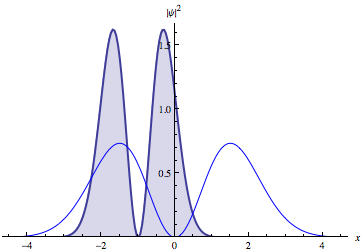
(a)

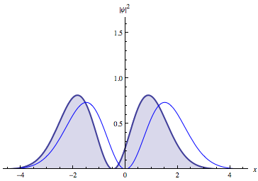
(b)

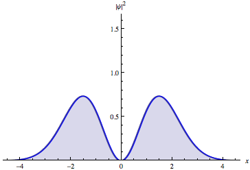
(c)

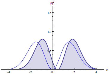
(d)

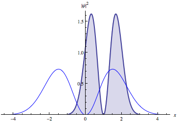
(e)

Figure 2. Subfigures (a)-(e) are a few stills taken from the mathematica movie animation [45]. Starting with (a) they denote the oscillating electron density (blue) of the first excited “dynamic harmonic state” of the time-dependent Schrödinger equation (1.1). These space oscillations complement (with the help of Mathematica) the corresponding “static” textbook solution (clear)[55]. (The color version of this figure is available only in the electronic edition.)

Example 3
The following animations simultaneously show the phase space oscillations of the electron density and the momentum probability distribution, according to the Heisenberg Uncertainty Principle, for the dynamic ground state $n=0$ with parameters $\alpha_{0}=\gamma_{0}=\varepsilon_{0}=\kappa_{0}=0$, $\beta_{0}=2/3$ and $\delta_{0}=3/2$:

In[3]:=$\displaystyle\mathrm{Animate}\Bigg{[}\text{Plot}\Bigg{[}\Bigg{\{}\frac{9\sqrt{2}\ e^{-\frac{18\left(2x+3\ \text{Cos}\left[\frac{1}{500}\pi(249+T)\right]\right)^{2}}{97+65\ \text{Cos}\left[\frac{1}{250}\pi(-1+T)\right]}}}{\sqrt{97+65\ \text{Cos}\left[\frac{1}{250}\pi(-1+T)\right]}}\ ,$

$\frac{9\sqrt{2}\ e^{\frac{18\left(-2x+3\ \text{Cos}\left[\frac{1}{500}\pi(-1+T)\right]\right)^{2}}{-97+65\ \text{Cos}\left[\frac{1}{250}\pi(-1+T)\right]}}}{\sqrt{97-65\ \text{Cos}\left[\frac{1}{250}\pi(-1+T)\right]}}\Bigg{\}}$, $\{x,-4.5,4.5\},\text{AxesLabel}\text{\ -$>$}$ $\{\{x,p\},\{(\text{Abs}[\psi]){}^{\wedge}2$,

$(\text{Abs}[a]){}^{\wedge}2\}\},\text{PlotRange}\to\{0,2.3\},\text{Filling}\to\{1\to\text{Bottom}\},\text{PlotStyle}\to\{\text{Thick},\text{Blue}\}\Bigg{]},\{T,1001\}\Bigg{]}$

Out[3]=

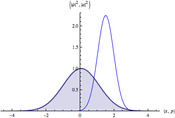
(a)

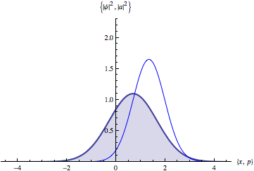
(b)

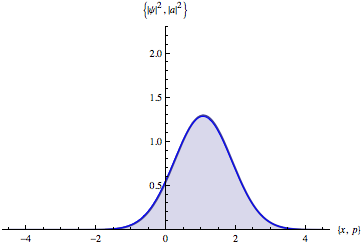
(c)

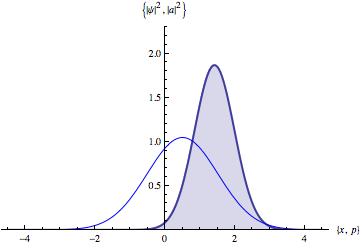
(d)

(e)

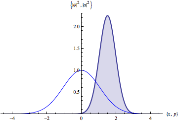
(f)

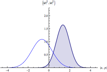
(g)

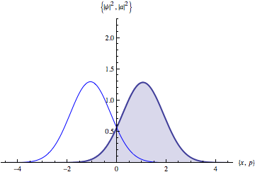
(h)

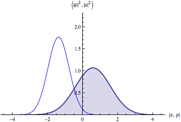
(i)

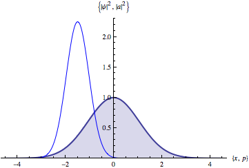
(j)

Figure 3. Subfigures (a)-(j) are a few stills taken from the mathematica movie animation [45]. Starting with (a) they denote simultaneous oscillations of electron density (blue) and probability distribution of momentum (clear) for the ground “dynamic harmonic state” of the time-dependent Schrödinger equation (1.1). These phase space oscillations complement (with the help of Mathematica) the corresponding “static” textbook solutions [23], [55]. (The color version of this figure is available only in the electronic edition.)

One immediately recognizes from these animations that the particle is the most localized at the turning points when its linear momentum is the least precisely determined, as required by the fundamental Heisenberg Uncertainty Principle [27] — The more precisely the position is determined, the less precisely the momentum is known in this instant, and vice versa (see also [8]). In the creator own words — “If the classical motion of the system is periodic, it may happen that the size of the wave packet at first undergoes only periodic changes” (see Ref. [27], p. 38).

According to (1.13), the corresponding expectation values are given by

$$\langle x\rangle= -\frac{1}{\beta_{0}}\left[\left(2\alpha_{0}\varepsilon_{0}-\beta_{0}\delta_{0}\right)\sin t+\varepsilon_{0}\cos t\right],\qquad\frac{d}{dt}\langle x\rangle=\langle p\rangle,$$ (A.1)

$$\langle p\rangle= -\frac{1}{\beta_{0}}\left[\left(2\alpha_{0}\varepsilon_{0}-\beta_{0}\delta_{0}\right)\cos t-\varepsilon_{0}\sin t\right],\qquad\frac{d}{dt}\langle p\rangle=-\langle x\rangle$$ (A.2)

with the initial data $\left.\langle x\rangle\right|_{t=0}=-\varepsilon_{0}/\beta_{0}$ and $\left.\langle p\rangle\right|_{t=0}=-\left(2\alpha_{0}\varepsilon_{0}-\beta_{0}\delta_{0}\right)/\beta_{0}.$ This provides a classical interpretation of our “hidden” parameters.

The expectation values $\langle x\rangle$ and $\langle p\rangle$ satisfy the classical equation for harmonic motion, $y^{\prime\prime}+y=0,$ with the total energy

$$\frac{1}{2}\left[\langle p\rangle^{2}+\langle x\rangle^{2}\right]=\frac{\left(2\alpha_{0}\varepsilon_{0}-\beta_{0}\delta_{0}\right)^{2}+\varepsilon_{0}^{2}}{2\beta_{0}^{2}}=\left.\frac{1}{2}\left[\langle p\rangle^{2}+\langle x\rangle^{2}\right]\right|_{t=0}.$$ (A.3)

For the standard deviations,

$$\langle\left(\Delta p\right)^{2}\rangle=\langle p^{2}\rangle-\langle p\rangle^{2}=\left(n+\frac{1}{2}\right)\dfrac{1+4\alpha_{0}^{2}+\beta_{0}^{4}+\left(4\alpha_{0}^{2}+\beta_{0}^{4}-1\right)\cos 2t-4\alpha_{0}\sin 2t}{2\beta_{0}^{2}},$$ (A.4)

$$\langle\left(\Delta x\right)^{2}\rangle=\langle x^{2}\rangle-\langle x\rangle^{2}=\left(n+\frac{1}{2}\right)\dfrac{1+4\alpha_{0}^{2}+\beta_{0}^{4}-\left(4\alpha_{0}^{2}+\beta_{0}^{4}-1\right)\cos 2t+4\alpha_{0}\sin 2t}{2\beta_{0}^{2}},$$ (A.5)

one gets

$$\langle\left(\Delta p\right)^{2}\rangle\langle\left(\Delta x\right)^{2}\rangle=\left(n+\frac{1}{2}\right)^{2}\frac{1}{4\beta_{0}^{4}}\left[\left(1+4\alpha_{0}^{2}+\beta_{0}^{4}\right)^{2}-\left(\left(4\alpha_{0}^{2}+\beta_{0}^{4}-1\right)\cos 2t-4\alpha_{0}\sin 2t\right)^{2}\right].$$ (A.6)

In the case of the Schrödinger solution [55], when $\alpha_{0}=\delta_{0}=\varepsilon_{0}=0$ and $\beta_{0}=1,$ we arrive at $\langle x\rangle=\langle p\rangle\equiv 0$ and

$$\langle\left(\Delta p\right)^{2}\rangle=\langle\left(\Delta x\right)^{2}\rangle=n+\frac{1}{2}$$ (A.7)

as presented in the textbooks [21], [23], [24], [29], [38], [47]. The dependence on the quantum number $n,$ which disappears from the Ehrenfest theorem [16], [27], is coming back at the level of the higher moments of the distribution.

According to (A.6),

$$\langle\left(\Delta p\right)^{2}\rangle\langle\left(\Delta x\right)^{2}\rangle=\left(n+\frac{1}{2}\right)^{2}\frac{1-4\alpha_{0}^{2}\sin^{2}2t}{\beta_{0}^{4}},$$ (A.8)

provided that $4\alpha_{0}^{2}+\beta_{0}^{4}=1,$ and the product is equal to $1/4,$ if $n=0$ and $\sin^{2}2t=1.$ These are conditions for the minimum-uncertainty squeezed states of the simple harmonic oscillator (see, for example, [29], [36]). For the coherent states $\alpha_{0}=0$ and $\beta_{0}=1,$ which describes a two-parameter family with the initial data $\left.\langle x\rangle\right|_{t=0}=-\varepsilon_{0}$ and $\left.\langle p\rangle\right|_{t=0}=\delta_{0}.$

The corresponding wave functions in the momentum representation are derived by the (inverse) Fourier transform of our solutions (1.2) and (1.3)–(1) in Appendix B. Moreover, in Appendix C, we explicitly present the action of the Schrödinger group on the wave functions of harmonic oscillators and elaborate on the corresponding eigenfunction expansion for the sake of ‘completeness’.

More examples are available in the authors’ websites.

Appendix B The Momentum Representation

For the wave functions in the momentum representation,

$$a_{n}\left(p,t\right)=\frac{1}{\sqrt{2\pi}}\int_{-\infty}^{\infty}e^{-ipx}\psi_{n}\left(x,t\right)\ dx,$$ (B.1)

the integral evaluation is similar to Ref. [39]. As a result, the functions $a_{n}\left(p,t\right)$ are of the same form (1.2)–(1), if $\psi_{n}\to a_{n}$ and $x\to p,$ with the initial data

$$\alpha_{1}=-\dfrac{\alpha_{0}}{4\alpha_{0}^{2}+\beta_{0}^{2}},\qquad\qquad\beta_{1}=\dfrac{\beta_{0}}{\sqrt{4\alpha_{0}^{2}+\beta_{0}^{2}}},$$ (B.2)

$$\gamma_{1}=\gamma_{0}+\dfrac{1}{2}\mathop{\mathrm{a}rccot}\dfrac{\beta_{0}^{2}}{2\alpha_{0}},\quad\mu_{1}=\mu_{0}\sqrt{4\alpha_{0}^{2}+\beta_{0}^{2}},$$ (B.3)

$$\delta_{1}=\dfrac{2\alpha_{0}\delta_{0}+\beta_{0}^{3}\varepsilon_{0}}{4\alpha_{0}^{2}+\beta_{0}^{2}},\qquad\quad\varepsilon_{1}=\dfrac{2\alpha_{0}\varepsilon_{0}-\beta_{0}\delta_{0}}{\sqrt{4\alpha_{0}^{2}+\beta_{0}^{2}}},$$ (B.4)

$$\kappa_{1}=\kappa_{0}+\dfrac{\alpha_{0}\left(\beta_{0}^{2}\varepsilon_{0}^{2}-\delta_{0}^{2}\right)+\beta_{0}^{3}\delta_{0}\varepsilon_{0}}{4\alpha_{0}^{2}+\beta_{0}^{2}}.$$ (B.5)

The calculation details are left to the reader [62] (see, for example, Ref. [23] for the classical case).

Appendix C The Schrödinger Group for Simple Harmonic Oscillators

The following substitution

$$\psi\left(x,t\right)=\frac{e^{i\left(\alpha\left(t\right)x^{2}+\delta\left(t\right)x+\kappa\left(t\right)\right)}}{\sqrt{\mu\left(t\right)}}\ \chi\left(\xi,\tau\right),$$ (C.1)

where relations (1.3)–(1) hold, transforms the time-dependent Schrödinger equation (1.1) into itself with respect to the new variables $\xi=\beta\left(t\right)x+\varepsilon\left(t\right)$ and $\tau=-\gamma\left(t\right)$ [50] (see also [44] and the references therein). A Mathematica verification can be found in Refs. [33] and [62].

The eigenfunction expansion of the “dynamic harmonic states” with respect to the standard “static”ones can be obtain in an obvious way (see, for example, [37] and [43] for similar integral evaluations, the details will appear elsewhere). The corresponding matrix elements define the representation of the Schrödinger group acting on the oscillator wave functions. (The structure of the Schrödinger group in two-dimensional space-time as a semidirect product of $SL\left(2,\mathbb{R}\right)$ and Weyl $W\left(1\right)$ groups is discussed, for example, in Refs. [7], [31] and [48].)

An explicit time evolution of the (bosonic field) creation and annihilation operators for the “dynamic harmonic (Fock) states”(with the embedded hidden Schrödinger group symmetry) can be easily derived from (1.13), (1.15) and (1.16). Applications to the quantization of electromagnetic fields are discussed in [35].

References

- [1] A. Akhiezer and V. B. Berestetskii, Quantum Electrodynamics, Interscience Publishers, New York, 1965.
- [2] V. Aldaya, F. Cossio, J. Guerrero and F. F. López-Ruiz, The quantum Arnold transformation, J. Phys. A: Math. Theor. 44 (2011), 065302 (19 pages).
- [3] R. L. Anderson, S. Kumei and C. E. Wulfman, Invariants of the equations of wave mechanics. I, Rev. Mex. Fís. 21 (1972), 1–33.
- [4] R. L. Anderson, S. Kumei and C. E. Wulfman, Invariants of the equations of wave mechanics. II One-particle Schrödinger equations, Rev. Mex. Fís. 21 (1972), 35–57.
- [5] M. V. Berry, Quantal phase factors accompanying adiabatic changes, Proc. Roy. Soc. London, A392 (1984) # 1802, 45–57.
- [6] M. V. Berry, Classical adiabatic angles and quantum adiabatic phase, J. Phys. A: Math. Gen. 18 (1985) # 1, 15–27.
- [7] C. P. Boyer, R. T. Sharp and P. Winternitz, Symmetry breaking interactions for the time dependent Schrödinger equation, J. Math. Phys. 17 (1976) #8, 1439–1451.
- [8] D. Cassidy, Uncertainty: The Life and Science of Werner Heisenberg, New York: W. H. Freeman, 1992; see also http://www.aip.org/history/heisenberg/p08.htm.
- [9] R. Cordero-Soto, R. M. López, E. Suazo and S. K. Suslov, Propagator of a charged particle with a spin in uniform magnetic and perpendicular electric fields, Lett. Math. Phys. 84 (2008) #2–3, 159–178.
- [10] R. Cordero-Soto, E. Suazo and S. K. Suslov, Quantum integrals of motion for variable quadratic Hamiltonians, Ann. Phys. 325 (2010) #9, 1884–1912.
- [11] E. A. Cornell and C. E. Wieman, Nobel Lecture: Bose–Einstein condensation in a dilute gase, the first 70 years and some recent experiments, Rev. Mod. Phys. 74 (2002) #3, 875–893.
- [12] V. V. Dodonov, Current status of dynamical Casimir effect, Physica Scripta 82 (2010) #3, 038105 (10 pp).
- [13] V. V. Dodonov, A. B. Klimov and D. E. Nikonov, Quantum phenomena in nonstationary media, Phys. Rev. A. 47 (1993) # 5, 4422–4429.
- [14] V. V. Dodonov, I. A. Malkin and V. I. Man’ko, Integrals of motion, Green functions, and coherent states of dynamical systems, Int. J. Theor. Phys. 14 (1975) # 1, 37–54.
- [15] V. V. Dodonov and V. I. Man’ko, Invariants and correlated states of nonstationary quantum systems, in: Invariants and the Evolution of Nonstationary Quantum Systems, Proceedings of Lebedev Physics Institute, vol. 183, pp. 71-181, Nauka, Moscow, 1987 [in Russian]; English translation published by Nova Science, Commack, New York, 1989, pp. 103-261.
- [16] P. Ehrenfest, Bemerkung über die angenäherte Gültigkeit der klassischen Mechanik innerhalb der Quantenmechanik, Zeitschrift für Physik A 45 (1927), 455–457.
- [17] V. P. Ermakov, Second-order differential equations. Conditions of complete integrability, Universita Izvestia Kiev, Series III 9 (1880), 1–25; see also Appl. Anal. Discrete Math. 2 (2008) #2, 123–145 for English translation of Ermakov’s original paper.
- [18] L. D. Faddeev, Feynman integrals for singular Lagrangians, Theoretical and Mathematical Physics 1 (1969) #1, 3–18 [in Russian].
- [19] P. O. Fedichev, Yu. Kagan, G. V. Shlyapnikov and J. T. M. Walraven, Influence of nearly resonant light on the scattering length in low-temperature atomic gases, Phys. Rev. Lett. 77 (1996) #14, 2913–2916.
- [20] R. P. Feynman and A. R. Hibbs, Quantum Mechanics and Path Integrals, McGraw–Hill, New York, 1965.
- [21] S. Flügge, Practical Quantum Mechanics, Springer–Verlag, Berlin, 1999.
- [22] T. Fujii, Sh. Matsuo, N. Hatakenaka, S. Kurihara and A. Zeilinger, Quantum circuit analog of the dynamical Casimir effect, Phys. Rev. B. 84 (2011) #17, 174521 (9 pages).
- [23] I. I. Gol’dman and V. D. Krivchenkov, Problems in Quantum Mechanics, Dover, New York, 1993.
- [24] J. Guerrero, and F. F. López-Ruiz, V. Aldaya and F. Cossio, Harmonic states for the free particle, J. Phys. A: Math. Theor. 44 (2011), 445307 (16pp); see also arXiv:1010.5525v3 [quant-ph] 1 Jul 2011.
- [25] C. H. Hagen, Scale and conformal transformations in Galilean-covariant field theory, Phys. Rev. D 5 (1972) #2, 377–388.
- [26] G. Harari, Ya. Ben-Aryeh and Ady Mann, Propagator for the general time-dependent harmonic oscillator with application to an ion trap, Phys. Rev. A 84 (2011) # 6, 062104 (4 pages).
- [27] W. Heisenberg, The Physical Principles of the Quantum Theory, University of Chicago Press, Chicago, 1930; Dover, New York, 1949.
- [28] W. Heisenberg, Physics and Philosophy: The Revolution in Modern Science, Ruskin House, Harper and Row, New York, 1958 (Lectures delivered at University of St. Andrews, Scotland, Winter 1955-56); see also http://www.aip.org/history/heisenberg/p13e.htm.
- [29] R. W. Henry and S. C. Glotzer, A squeezed-state primer, Am. J. Phys. 56 (1988) #4, 318–328.
- [30] R. Jackiw, Dynamical symmetry of the magnetic monopole, Ann. Phys. 129 (1980), 183–200.
- [31] E. G. Kalnins and W. Miller, Lie theory and separation of variables. 5. The equations and J. Math. Phys. 15 (1974) #10, 1728–1737.
- [32] Yu. S. Kivshar, T. J. Alexander and S. K. Turitsyn, Nonlinear modes of a macroscopic quantum oscillator, Phys. Lett. A 278 (2001) #1, 225–230.
- [33] C. Koutschan, http://hahn.la.asu.edu/~suslov/curres/index.htm; see Mathematica notebook: Koutschan.nb; see also http://www.risc.jku.at/people/ckoutsch/pekeris/
- [34] C. Koutschan and D. Zeilberger. The 1958 Pekeris-Accad-WEIZAC Ground-Breaking Collaboration that computed Ground States of Two-Electron Atoms (and its 2010 Redux), Math. Intelligencer 33 (2011) #2, 52–57.
- [35] S. I. Kryuchkov and S. K. Suslov, On the problem of electromagnetic-field quantization, under preparation.
- [36] S. I. Kryuchkov, S. K. Suslov and J. M. Vega-Guzmán, The minimum-uncertainty squeezed states for the simple harmonic oscillator, under preparation.
- [37] N. Lanfear and S. K. Suslov, The time-dependent Schrödinger equation, Riccati equation and Airy functions, arXiv:0903.3608v5 [math-ph] 22 Apr 2009.
- [38] L. D. Landau and E. M. Lifshitz, Quantum Mechanics: Nonrelativistic Theory, Pergamon Press, Oxford, 1977.
- [39] N. Lanfear, R. M. López and S. K. Suslov, Exact wave functions for generalized harmonic oscillators, Journal of Russian Laser Research 32 (2011) #4, 352–361; see also arXiv:11002.5119v2 [math-ph] 20 Jul 2011.
- [40] N. Lanfear, F. F. López-Ruiz, S. K. Suslov and J. M. Vega-Guzmán, Coherent states for generalized harmonic oscillators, under preparation.
- [41] P. G. L. Leach and K. Andriopoulos, The Ermakov equation: a commentary, Appl. Anal. Discrete Math. 2 (2008) #2, 146–157.
- [42] H. R. Lewis, Jr., and W. B. Riesenfeld, An exact quantum theory of the time-dependent harmonic oscillator and of a charged particle in a time-dependent electromagnetic field, J. Math. Phys. 10 (1969) #8, 1458–1473.
- [43] R. M. López and S. K. Suslov, The Cauchy problem for a forced harmonic oscillator, Revista Mexicana de Física, 55 (2009) #2, 195–215; see also arXiv:0707.1902v8 [math-ph] 27 Dec 2007.
- [44] R. M. López, S. K. Suslov and J. M. Vega-Guzmán, On the harmonic oscillator group, arXiv:1111.5569v2 [math-ph] 4 Dec 2011.
- [45] R. M. López, S. K. Suslov and J. M. Vega-Guzmán, http://hahn.la.asu.edu/~suslov/curres/index.htm; see Mathematica notebook: HarmonicOscillatorGroup.nb
- [46] I. A. Malkin and V. I. Man’ko, Dynamical Symmetries and Coherent States of Quantum System, Nauka, Moscow, 1979 [in Russian].
- [47] E. Merzbacher, Quantum Mechanics, third edition, John Wiley & Sons, New York, 1998.
- [48] W. Miller, Jr., Symmetry and Separation of Variables, Encyclopedia of Mathematics and Its Applications, Vol. 4, Addison–Wesley Publishing Company, Reading etc, 1977.
- [49] U. Niederer, The maximal kinematical invariance group of the free Schrödinger equations, Helv. Phys. Acta 45 (1972), 802–810.
- [50] U. Niederer, The maximal kinematical invariance group of the harmonic oscillator, Helv. Phys. Acta 46 (1973), 191–200.
- [51] A. F. Nikiforov, S. K. Suslov, and V. B. Uvarov, Classical Orthogonal Polynomials of a Discrete Variable, Springer–Verlag, Berlin, New York, 1991.
- [52] L. Pitaevskii and S. Stringari, Bose–Einstein Condensation, Oxford University Press, Oxford, 2003.
- [53] S. Rosencrans, Perturbation algebra of an elliptic operator, J. Math. Anal. Appl. 56 (1976) #2, 317–329.
- [54] B. Sanborn, S. K. Suslov and L. Vinet, Dynamic invariants and Berry’s phase for generalized driven harmonic oscillators, Journal of Russian Laser Research 32 (2011) #5, 486–494; see also arXiv:1108.5144v1 [math-ph] 25 Aug 2011.
- [55] E. Schrödinger, Der stetige Übergang von der Mikro-zur Makro Mechanik, Die Naturwissenshaften, 14 (1926), 664–666; see also http://www.nobelprize.org/nobel_prizes/physics/laureates/1933/schrodinger-bio.html and http://www.zbp.univie.ac.at/schrodinger/euebersicht.htm.
- [56] E. Suazo and S. K. Suslov, Soliton-like solutions for nonlinear Schrödinger equation with variable quadratic Hamiltonians, arXiv:1010.2504v4 [math-ph] 24 Nov 2010.
- [57] E. Suazo, S. K. Suslov and J. M. Vega-Guzmán, The Riccati equation and a diffusion-type equation, New York J. Math. 17a (2011), 225–244.
- [58] E. Suazo, S. K. Suslov and J. M. Vega-Guzmán, The Riccati system and a diffusion-type equation, arXiv: 1102.4630v1 [math-ph] 22 Feb 2011.
- [59] S. K. Suslov, Dynamical invariants for variable quadratic Hamiltonians, Physica Scripta 81 (2010) #5, 055006 (11 pp); see also arXiv:1002.0144v6 [math-ph] 11 Mar 2010.
- [60] S. K. Suslov, On integrability of nonautonomous nonlinear Schrödinger equations, to appear in Proc. Amer. Math. Soc.; see also arXiv:1012.3661v3 [math-ph] 16 Apr 2011.
- [61] S. K. Suslov, The Berry phase for simple harmonic oscillators, arXiv:1112.2418v2 [quant-ph] 14 Dec 2011.
- [62] S. K. Suslov, http://hahn.la.asu.edu/~suslov/curres/index.htm; see Mathematica notebooks: BerrySummary.nb, Fourier.nb and Heisenberg.nb.
- [63] L. Vinet and A. Zhedanov, Representations of the Schrödinger group and matrix orthogonal polynomials, J. Phys. A: Math. Theor. 44 (2011) #35, 355201 (28 pages).
- [64] K. B. Wolf, On time-dependent quadratic Hamiltonians, SIAM J. Appl. Math. 40 (1981) #3, 419–431.
- [65] K-H. Yeon, K-K. Lee, Ch-I. Um, T. F. George and L. N. Pandey, Exact quantum theory of a time-dependent bound Hamiltonian systems, Phys. Rev. A 48 (1993) # 4, 2716–2720.
- [66] H. P. Yuen, Two-photon coherent states of the radiation field, Phys. Rev. A 13 (1976) #6, 2226–2243.
- [67] J. Q. You and F. Nori, Atomic physics and quantum optics using superconducting circuits, Nature 474 (2011), 589–597.
- [68] A. V. Zhukov, Exact quantum theory of a time-dependent system with quadratic hamiltonian, Phys. Lett. A 256 (1999) #5–6, 325–328.