Common Methods of Stellar Spectra Analysis and their Support in VO

Abstract

The proper scientific analysis of a large amount of stellar spectra requires certain capabilities of the analysing tool (e.g. precise semi-automatic fitting for normalisation of the continuum or line-list assisted measurement of spectral lines) as well as flexible list-driven datafile handling.

While most astronomical legacy packages comprise powerful analysing and data management features allowing rapid processing of quite complex data, current VO tools are lacking support of even basic capabilities commonly used in stellar spectroscopy.

Especially the high resolution optical spectroscopy of stars with rapid line profile variations or of those with complicated emission profiles benefits from a number of specific methods unsupported in todays Virtual Observatory (VO) tools and even lacking definition in VO spectral protocols.

In our contribution we identify these techniques, describe their possible implementations and finally give a short overview of several VO-compatible tools emphasising their deficiencies and comparing with the capabilities of common legacy packages.

1 Introduction

There is a wealth of calibrated astronomical spectra accessible in current data archives, however most of them are not suitable for direct physical analysis. Being prereduced by some automatic pipeline or individually by manual reduction, they are mostly stored in archives in form of FITS file or ASCII table as the relation of intensity in arbitrary numbers (instrumental counts, digital numbers etc.) and wavelength (or frequency).

The scientific analysis of such spectra requires further processing by the variety of different methods. In certain studies a huge number of spectra has to be collected from different servers (e.g. in different spectral regions ) and transformed into common units. Often the transformed spectra or variables measured in them (e.g. equivalent width) are visually inspected as the time series ordered by time of observation or by the orbital phase.

The tools with built-in VO protocols may considerably increase the efficiency of astronomical analysis by eliminating the data collection, aggregation and conversion and by allowing the astronomer to fully concentrate on the visual properties of data (e.g. searching the variability of line profiles or constructing the radial velocity curve). To be accepted quickly by the wide astronomical community a number of methods and recipes has to be implemented in a manner very similar to the current legacy applications. We attempted to identify the most useful methods and give hints for their implementation in VO clients.

2 Common methods of astronomical spectroscopic analysis

2.1 Rectification

Usually the first step in data analysis is the rectification of the spectrum (normalisation of the continuum to level 1.0). Although absolutely flux-calibrated spectrum is common for space instruments, it is rather exceptional in ground-based optical stellar spectroscopy (used mainly for determination of spectral type from low resolution spectra).

Usually, simple polynomials of low degree are applied for this purpose but there is a number of problems that have to be addressed:

Anchoring of edges

- all fitting polynomials have to be correctly anchored at the edges to work well. However in many cases the edge of the chip has a different behaviour than the middle. Usually the edges show rapid decline in intensity due to the vignetting of optics or due to lower detector quantum efficiency on low resolution spectra covering whole visible range both at UV and IR regions. Such curve with flat middle and rapidly falling edges is very difficult to fit with low order polynomials.

Flexibility of fitting curve

- The big problem of fitting curves is connected with their flexibility. The curve should be rigid enough to bridge consistently the continuum gap over strong wide lines (Hydrogen, Helium) and flexible enough the fit well the changes in curvature of continuum. This is especially important for normalising spectra of hot stars (strong He and Hydrogen Balmer lines) stars or rapidly rotating stars with broadened lines. Too high orders of fit tend to enter into the line, low order do not copy the tilt of continua at the edges well.

Majority of legacy spectral tools use Chebyschev or Legendre polynomials and cubic splines (e.g. IRAF splot, MIDAS XAlice or Starlink DIPSO). What is needed is a fitting routine that mimics the freehand drawing of the experienced astronomer. One of the little known but very powerful procedure is INTEP (Hill, 1982), which uses Hermittean polynomials, It has been successfully used many years for normalising spectra of Be stars in SPEFO (Škoda, 1996) and recently implemented in SPLAT-VO. Special attention was given to freehand drawing algorithms by Akima (1970). His procedure is implemented in SPLAT-VO as well.

Range of data points included into fit

Some programs (e.g. IRAF splot) allow to fit only the existing data points but some regions (e.g. wide lines) may be excluded by giving the number of distinct regions. The more flexible approach (e.g. in SPEFO, SPLAT-VO) is the possibility of placing individual control points everywhere (e.g. above the apparent continuum). The extrapolation of fitting line beyond the available data range can help to decide about the best parameters (polynomial order, number of spline segments) from its global behaviour (smoothness of curve and asymptotic approach to the particular value).

The problem of physical continuum

The continuum may be not seen on some objects so it cannot be fitted using the available data points. Problem in cooler stars is to locate the real position of the continuum - it may not be present at all due to severe blend of lines or molecular bands - then a model is needed.

It is extremely difficult to normalise certain stars with unusual profiles — like stars with rapidly expanding envelopes (post-AGB outbursts, nova shells), having strong emission lines with P-Cyg profile dominating whole spectrum.

For some stars with extremely strong emission lines (e.g. some Be and B[e] stars) the dynamic range of 16-bit ADC is insufficient to obtain the unsaturated line together with a well exposed continuum. Often the continuum is hidden in background noise.

Normalising echelle spectra

A really challenging problem (which had not yet been solved fully) is the normalisation of echelle spectra - especially with wide absorption lines or complicated profiles (P Cyg, Be stars). Some wide lines may span several echelle orders and so the individual orders have to be precisely unblazed and then merged. This problem is very complex, depending on construction of individual spectrograph, the observation strategy etc. See Škoda & Hensberge (2003), Škoda & Šlechta (2004), Prugniel & Soubiran (2001) or Erspamer & North (2002).

$\chi^{2}$ fitting procedures

The more advanced way of normalising is the least squares fitting based on some theoretical model. It is very popular in radioastronomy and X-ray astronomy ( XSPEC ) rather for estimation of the global SED fit parameters (usually only as combination of several simple power law functions). Quite useful in optical spectroscopy is the usage of appropriate synthetic spectrum to find the real continuum in data. The implementation of such a procedure in VO tools could call the Theory VO (TVO) servers to get correct models (e.g. Kurucz) and perhaps to improve the models by recomputing on the GRID in a iterative way. Unfortunately for many interesting objects models (even spectral classification) are only speculative.

2.2 Simple visual comparison

A lot of the information about the behaviour of astronomical objects can be estimated just by a visual inspection of a spectrum (spectral type, peculiarity, emission) or a time series of spectra (pulsations, binarity). The basic method is the overplotting of many spectra in the same units and scale. It may be very efficient with VO-enabled tools obtaining the number of spectra cached immediately from VO spectral servers through Simple Spectra Access Protocol (SSAP). There are many possibilities of plots:

• Overplotting spectra of different objects in the same region

• Overplotting the same object in different wavelength ranges (from X or UV over IR to radio). If the spectra are flux calibrated, it is the construction of spectra energy distribution (SED).

• Comparison of observation with models (rotationally broadened theoretical spectra)

• Plot of different lines overplotted in radial velocity scale may give he information about physical structure (e.g. for study of kinetic behaviour of different elements in expanding envelopes (Kipper et al., 2004)).

2.3 Study of line profile variations

The high resolution spectra with high SNR may reveal on some objects small variations of the profile of spectral lines. The study of LPV requires many (even hundreds) of spectra to be overplotted to see the changes well. Sometimes the animation of changes in individual spectral line is very impressive. The low SNR data should be removed not to spoil the image. To identify them some form of colour highlighting should be implemented together with single-stroke delete command to remove it from plotting list. Such a plot is helpful in asteroseismology or for estimating changes in stellar winds.

2.4 Dynamical spectrum

It is sometimes called the gray representation or trailed spectrum. The basic idea is to find the small time-dependent deviations of individual line profiles from some average.

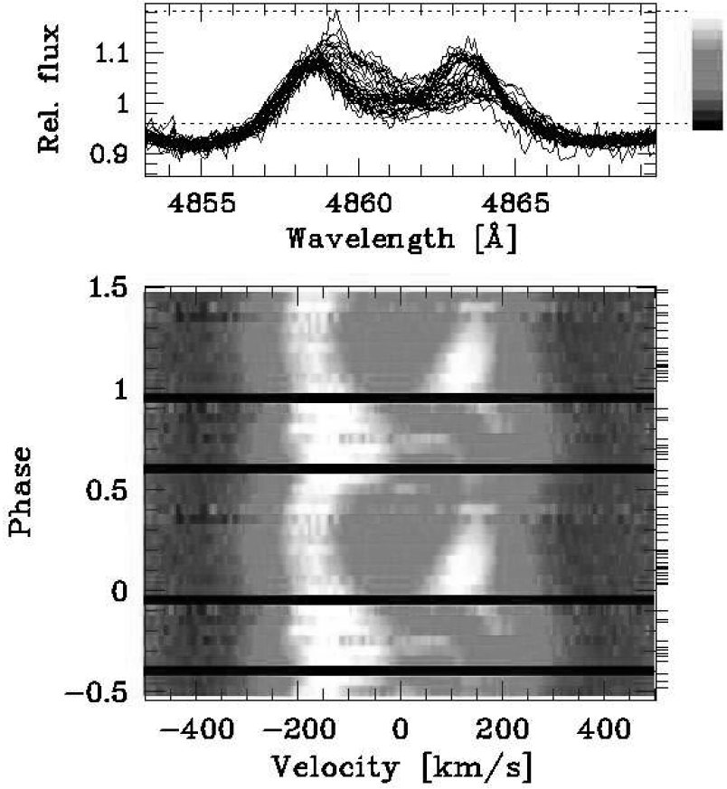
Figure 1: Dynamical spectrum of H$\beta$ line profile variability of 59 Cyg. Residuals from average profile of 38 spectra are binned to 20 phase bins corresponding to period 28.192 days. Two expanded cycles shown for clarity. Individual profiles are overplotted above. After Maintz (2003)

First the average of many high dispersion high SNR spectra (with removal of outliers) is prepared (called template spectrum). Then each individual spectrum in time series is either divided by the template (quotient spectrum) or the template is subtracted from it (the differential spectrum). The group of similar resulting intensities is given the same colour or level of gray. See Fig. 1 and Fig. 2. More examples may be found e.g. in de Jong et al. (1999), Maintz (2003) or Uytterhoeven (2004).

The result is drawn in 2D image where on horizontal axis is a wavelength in the line profile or corresponding RV relative to laboratory wavelength, on the vertical axis the time of middle of observation (in HJD) or the circular phase when the data are folded with certain period. Valuable are interactive features, like zoom of whole dataset, removal of bad spectra from series, adjustable colour cuts and look-up-tables etc.

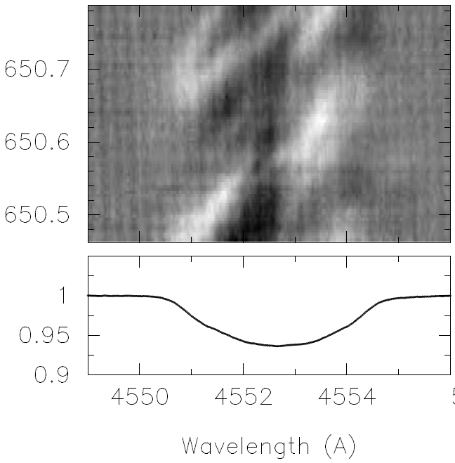
Figure 2: Dynamical spectrum of SiIII line profile variability of $\lambda$ Sco. The average profile of 8 observing nights was used as a template shown below the panels. After Uytterhoeven (2004)

2.5 Measurement of radial velocity and higher moments of line profile

The one of the important information received from spectrum is the radial velocity of the object - e.g. the binarity can be revealed , or the possession of extrasolar planet. RV is sometimes presented as zero-th moment of the spectral line profile. The higher moments of the line profile are important as well. The first moment is equivalent width. The combination of higher moments of line profile is a one of the possible ways of determination of non radial pulsation modes numbers $l,m$ (Aerts et al., 1992).

RV by fitting profiles

This is a most common method implemented in every spectral package. The data points in given range of line profile are directly fitted by Gauss, Lorentz or Voight function. At least rough normalisation is required. Problems occur in case of asymmetric and complicated profiles (e.g. P-Cyg type).

RV estimation by profile mirroring

It is a method used already many years ago in oscilloscopic comparators. The goal is to estimate the best match of the line profile and its flipped image (mirror around y axis in certain wavelength). The mirrored profile is being shifted interactively until the best match is assessed. This method (as implemented in SPEFO) has been successfully used for measurement of RV of stars with very complicated emission profiles (e.g. Be stars, luminous blue variables with strong wind, nova outbursts).

The implementation should allow the region of interest (wing or core) in vertical and the width of flipped area in horizontal direction to be easily adjustable. The reference line position is best taken from given linelist providing rest wavelength. The strength of this method lies in the capability of measuring the match of core and match of wings separately. See Fig. 3. More examples are given in Parimucha & Škoda (2006). This allows to study a different physics of particular line-forming regions (e.g. shells, jets, stellar winds).

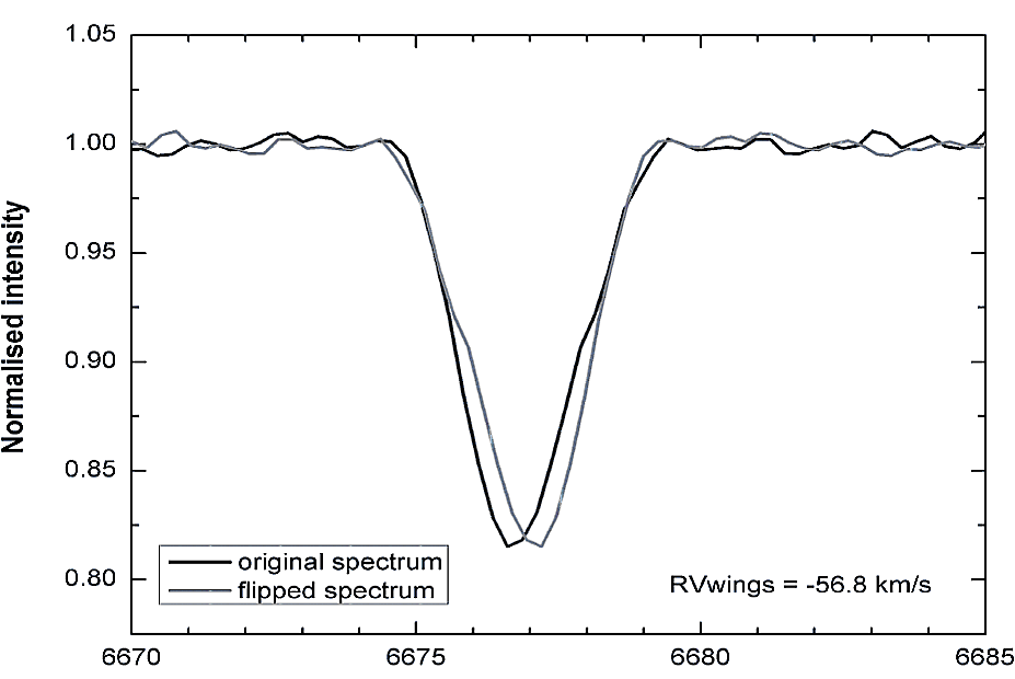
Figure 3: The estimation of RV by mirroring of profile. This case shows the match of line wings.

There is a close connection with bisector analysis, when the region of match is controlled in different levels of depth of the line profile.

RV by cross correlation

It is often used to measure the RV of late type stars with known spectral classification. It does not measure RV of individual 9iu lines but a RV shift of the whole spectrum. Many sharp lines are required and a good template (usually a synthetic spectrum convolved to the similar resolution and rotational broadening as observed one) (Barton et al., 2000). Continuum normalisation is critical.

Many legacy applications (IRAF package xrv and RVSAO, standalone program DAOSPEC, MIDAS task XCORRELATE …). Often used for searching extrasolar planets (cross-correlation with Iodine cell spectrum). The cross-correlation is an ideal method for measurement of RV in echelle spectra (many lines in different spectral regions may be combined together).

2.6 Measurement of equivalent width

The measurement of equivalent width (EW) of a given line needs the determination of area bordered by line profile and the continuum. This area is transformed to the rectangular line with the depth of 1.0. The width of this rectangle is called equivalent width. Emission lines by definition have negative EW.

The measurement is sensitive to continuum placement. The extremely shallow lines give large error in EW (Vrancken et al., 1997). EW are often used in abundance analysis. A good check of correct normalisation is the comparison of EW of spectral lines of the same element in different spectral regions (Hensberge et al., 2000).

The comparison of EW measured in spectrum of point-like solar system bodies (minor planets) with high resolution solar spectrum from solar telescopes gives the information about the intrinsic spectrograph properties (stray light) and quality of pipeline reduction (Erspamer & North, 2002).

2.7 Bisector analysis

It is a method describing quantitatively the tiny asymmetry or subtle changes in line profiles. It is easily done by marking the middle of horizontal cuts of profile in different line depths. The line connecting such points (called bisector) is then zoomed in horizontal (wavelength or RV) direction. See Fig. 4.

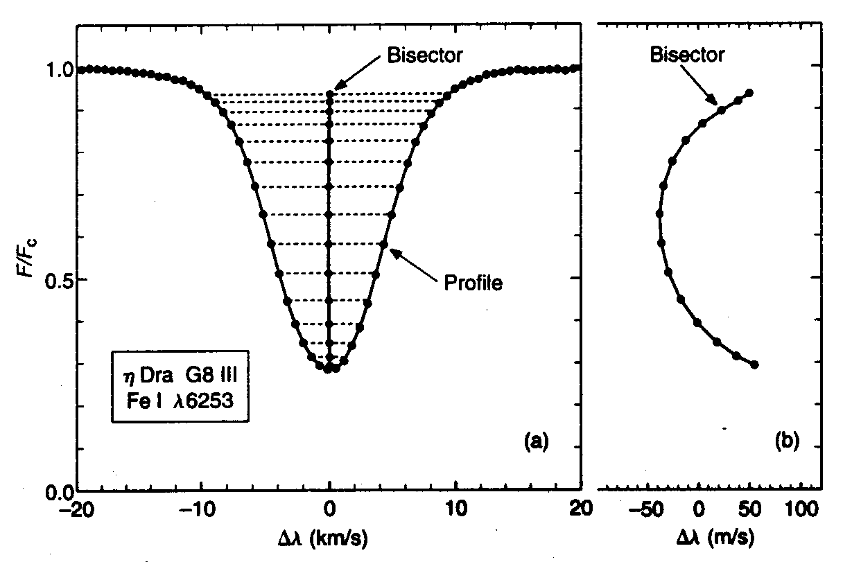
Figure 4: The construction of bisector of line profile (left panel) and the zoomed bisector (right panel). From Gray (1982).

The characteristic shape of bisector gives the information about turbulence fields (e.g. convection) in stellar photosphere, characterised by the value of micro-turbulent velocity (Gray, 1982, 2005) or about other processes causing the tiny profile asymmetry. It has been used successfully for searching of extrasolar planets (Povich et al., 2001) or in asteroseismology. Requires high resolution (echelle) and high SNR normalised spectra. Still some smoothing of edges in steeply declining line wings is helpful (Martínez Fiorenzano et al., 2005).

2.8 Rotational broadening

Before comparing the synthetic spectrum with observed, the rotational broadening has to be applied, especially for rapid rotators. The estimate of rotational velocity $v\sin i$ is thus obtained.

Although simple formula of convolution with parabolic kernel has been mostly used, the precise computation is very complicated (the problem of limb darkening) especially in non-LTE case (Hadrava & Kubát, 2003).

Sometimes a Fourier transformation of a line profile (with high SNR) is applied to get the first estimate of rotational velocity (Gavrilović & Jankov, 2007).

2.9 Period Analysis

One of the most popular methods used in astronomy is the period analysis. Its aim is to find the hidden periods of variability of given object. Sometimes this period can be identified with some physical mechanism (e.g. orbital period of binaries, rotational modulation or pulsations). Wide range of objects show the multi-periodicity on various time scales (e.g. binary with pulsating components). Ones the suspected period is found, the data may be folded accordingly, plotted in circular phase corresponding this period. Very helpful is a interactive capability of showing data folded while selecting different peaks at the periodogram.

The number of methods applied is large. but there are several very popular in astronomy:

• Folding techniques: Phase dispersion minimisation PDM (Stellingwerf, 1978).

• Fourier methods: Widely used algorithm CLEAN (Roberts et al., 1987) or its modified Lomb-Scargle version (Lomb, 1976; Scargle, 1989).

• Periodogram of RV of bisector (sometimes called local RV). The periods in position of bisectors in different line depths may give an idea where the profile is affected by given non radial pulsation mode (Koubský et al., 2007).

• Periodogram of line profile. It is a kind of gray representation with period on vertical axis and the zoomed line profile on horizontal. See Fig. 5. Works well for analysis of multi-periodical non-radial pulsations (de Jong et al., 1999).

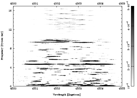
Figure 5: Example of 2D periodogram of SiIII 4552 Å line profile variability of $\lambda$ Sco. After Uytterhoeven (2004).

3 Complex processing methods

For the complex techniques given below, a lot of additional information is required in addition to spectral data. Programs require complicated configuration files in given format and some interactive trials to find the best results using the output from recent run as input to next one. They are written often in FORTRAN without graphical interface or even the plotting capabilities. They are designed for batch runs driven by parameter files. Their application is limited to special cases of certain objects with appropriate physical properties.

3.1 Doppler imaging

It was introduced by Vogt & Penrod (1983a) as a method allowing the surface mapping of stellar spots. First test were done on stars of RS CVn type and on $\zeta$ Oph (Vogt & Penrod, 1983b). Works well on rapid rotators and needs a high resolution spectra with very high SNR (300–500). Tho whole rotational period should be covered well, better several times. When all the requirements are met, the map of surface features (spots, nodes of non radial pulsations) is obtained with very high accuracy.

3.2 Doppler tomography

It was introduced by Marsh & Horne (1988) for mapping the distribution of emitting circumstellar matter in binary system. One of successful application gave a picture of accretion jets in Algols (Richards, 2004). It uses trailed spectrum in velocity scale. The result is 2D image in velocity space. The transformation of radial velocity space to coordinate space is ambiguous, which causes problems in interpretation of Doppler tomograms.

3.3 Spectra disentangling

This method allows to disentangle the spectra of individual stars in binary or multiple systems even in case of heavy blending of lines. It supposes the changes in line profile are caused only by combination of Doppler shifted components (no intrinsic variability of star). The best solution of orbital parameters and disentangled line profiles of individual stellar components are found by least square global minimisation. Automatically removes the telluric lines with great precision. Requires good orbital coverage and the estimate of orbital parameters. Two approaches exist:

Wavelength space disentangling

developed by Bagnuolo & Gies (1991) and improved by Simon & Sturm (1994). It needs a large memory to store sparse matrices, requires large computing power. Gives more reliable results

Fourier space disentangling

introduced by Hadrava (1995) and Hadrava (1997) in program KOREL. Another program available today (still based on KOREL ideas) is FDBINARY (Ilijic et al., 2004). They work in Fourier space, and transform the wavelengths into $\ln\,\lambda$. They solve a small amount of linear equations, so they are memory savvy and can be run on even small computer. The method, however, requires perfect continuum fit (difficult to achieve at merged echelle spectra). On unreliably rectified spectra strange artifacts may appear (Ilijic et al., 2004).

4 VO-enabled tools

Although there is a number of various tools written for the analysis of spectra of astronomical objects (e.g IRAF, MIDAS, Starlink packages splot, spectool, DIPSO, XALICE as well as numerous single-purpose C, FORTRAN and IDL routines), the number of modern tools understanding the VO protocols (especially spectra access protocol - SSAP) is still very low. We are giving a brief overview of their capabilities and status of development at the time of the submission of these proceedings (May 2007).

4.1 VOSpec

• Current version 2.5

• http://esavo.esa.int/vospec/

• Developed at ESA

• Very simple (mainly for building SED)

• Polynomial and Gaussian fits only

• Blackbody fit

• No RV measurement built-in

• No complex operations with spectra allowed

• It can be called directly from VizieR

• Can work with linelists through Simple Line Access Protocol (SLAP)

• Theoretical VO (TVO) supported (synthetic spectra: Kurucz, disks)

• Rapid development

• Integration of some methods in users own program possible

• JAVA applet

• Contains PLASTIC VO-interoperability layer

• Dereddening of extragalactic objects built-in

• Support of dimensional equations for units (DIMEQ, SCALEQ)

• Rather complicated view of users data - needs to create SSA wrapper and prepare VOTable even for one simple FITS spectrum before viewing

4.2 SpecView

• Current version 2.13

• http://www.stsci.edu/resources/software_hardware/specview

• It is available as JAVA applet or stand-alone application

• Developed and supported by STScI

• Understands a number of formats from HST instruments and most NASA/ESA satellites

• Understands general FITS in form of binary tables

• Does not handle simple 1D FITS (binary images with CDELT, CRVAL)

• Easy work is with local data (if binary or ASCII tables)

• Well tailored for practical spectral analysis

• Powerful linelists (many included)

• Fitting of models by $\chi^{2}$ — even user models may be constructed

• Built-in number of standard stars spectra and models for various physical conditions

• Whole Kurucz library of spectra available for immediate display.

• Only simple polynomials for visual fit available

• Dereddening, CLOUDY models built-in

• Proper error propagation of fitted values

• Support of dimensional equations

• Does not support PLASTIC

4.3 SPLAT-VO

• Current version 3.7

• http://star-www.dur.ac.uk/ pdraper/splat/splat-vo/

• Supported by JCMT after closing Starlink

• Most advanced for stellar astronomy (fitting by freehand drawing, INTEP)

• RV measurement - both Gaussian fit and mirroring

• Custom line list for individual spectra available

• Wavelet analysis

• Full featured data and editor and spreadsheet

• Publication quality output, powerful plotting options, annotations

• Supported PLASTIC

• Reads 1D FITS image files (e.g. rebinned IRAF multispec files)

• Asynchronous SSAP queries

4.4 Period04

• Current version 1.0.2

• http://www.univie.ac.at/tops/Period04/

• Its predecessor was widely used Period98

• Period04 is rewritten in Java (and partly C)

• Needs formatted text files

• VO-interface not supported, only local VOTable files

• Several period finding methods built-in

• Can handle even the regular period shifts

4.5 FROG

• Part of Starlink Java package

• Included in last JCMT Starlink release (Hokulei)

• http://www.jach.hawaii.edu/software/starlink/

• VO-protocols built-in

• Almost same capabilities as Period04

• Unclear status of development after closing Starlink - all the links to documentation and files are now wrong

• Last version since 2004 - no further development noticed

• The period searching engine available remotely as a SOAP service

• Web service for Fourier transform

• Collaborates with TOPCAT, but not PLASTIC

• Easy but powerful for doing period analysis in VO environment

5 Implementation strategies

As was shown above, the current VO-enabled tools are already very flexible to allow the large part of analysis of astronomical spectra to be directly performed in the VO environment using the data through SSAP. However, many “classical ” astronomers, working mostly with middle and high resolution stellar spectra in visual wavelengths, will not use these tools until most of the features described earlier are implemented.

The functional behaviour of such implementations is very important as well. To be quickly adopted by the conservative part of stellar community, the tool should be self-learning: it should allow interactive work with one or couple of spectra to adjust the parameters (ranges for measurement, degree of fitting polynomials etc.). But after tuning its behaviour it should be able to apply the same recipes to large number of spectra with similar characteristics. The very promising way how to do it is the concept of workflows.

There is a important question where to put the engine for spectral analysis. All tools today re the JAVA applications running as VO-client on astronomer’s computer. Adding more features (new methods of data processing) requires the new version of client to be downloaded and installed. Despite the possible automatic installation through Java WebStart there is a serious problem of size and complexity of such tool. Although the new functions could be added as client plugins (similar to Firefox plugins), we do not consider such a solution to be prospective on a long-term scale as it is against the original concept of VO. VO has been usually advertised as a facility allowing seamless federation of all distributed data archives and computing resources providing data processing services through Web Services.

Certain amount of processing power should be thus left at the data providing servers. It may perform some simple operations before sending the spectrum to the client. For example it may transform the units (both wavelength and flux), cut out only the requested wavelengths (e.g. 20 A long section centred around H$\alpha$) or even the server might perform the normalisation of spectrum by approximate continuum fit - either computed using given parameters of fit or just applying the fit included in calibrated spectrum (some reduction programs produce spectra in format containing both the unrectified spectrum with intensity in ADU and the continuum fit described by type and degree of polynomials and list of control points).

But most of complicated processing (e.g. spectra disentangling, Doppler tomography, period analysis, should be rather performed on dedicated problem-oriented servers using Web Services or similar technology. It is, however, difficult to convince the authors of powerful legacy (mostly FORTRAN) applications to re-implement them according to requirements of VO infrastructure (they do not know the JAVA, VO protocols etc.) and it is dangerous to ask the software developer to blindly re-code such a applications without detailed knowledge of the employed mathematical methods (including their bottlenecks and week points).

Thus the only feasible way how to create most of such Web Services is to create the VO-compatible wrappers calling the legacy application as it was designed using its native input and output file format. The collaboration with authors is important anyway.

The utilisation of dedicated servers allows easy extension of processing capabilities by adding another service to the same server (e.g. by adding Apache-like server module) or by installing new dedicated server. The natural way of solving complicated computing demanding problems is to deploy such services on GRID.

There are still tasks in astronomical spectra analysis requiring visual interaction (e.g. precise fitting of complicated continuum, measurement of RV by profile mirroring or adjusting the colour scale of dynamical spectrum to strengthen particular feature in it). Such (usually simple) procedures may be left on the client side. Today, when there is a very few applications written in form of Web Services (to be deployed on server side), the extension of client capabilities seems to be the easiest solution even for some server-oriented tasks (e.g. the cutout of selected spectral region).

6 Conclusions

Astronomical spectroscopy uses a wide range of techniques with different level of complexity to achieve its final goal — to estimate the most precise and reliable information about celestial objects. The large part of spectroscopic analysis today has been accomplished by several independent non VO-compatible legacy packages, where each works with different local files in its own data format. Analysis of large number of spectra is thus very tedious work requiring good data bookkeeping.

Accomplishing the analysis in VO infrastructure may benefit from automatic aggregation of distributed archive resources (e.g. the multispectral research), seamless on-the-fly data conversion, common interoperability of all tools (using PLASTIC protocol) and powerful graphical visualisation of measured and derived quantities (e.g. in VOPlot or Mirage).

By introduction of modern VO-aware tools into the astronomical spectral analysis a remarkable increase of effectivity of astronomical research can be achieved.

References

- Aerts et al. (1992) Aerts, C., de Pauw, M., & Waelkens, C. 1992, A&A, 266, 294
- Akima (1970) Akima, H. 1970, Journal Assoc. Comp. Mach., 17(4), 589
- Bagnuolo & Gies (1991) Bagnuolo, W. G., Jr., & Gies, D. R. 1991, ApJ, 376, 266
- Barton et al. (2000) Barton, E. J., Kannappan, S. J., Kurtz, M. J., & Geller, M. J. 2000, PASP, 112, 367
- de Jong et al. (1999) de Jong, J. A., Henrichs, H. F., Schrijvers, C., Gies, D. R., Telting, J. H., Kaper, L., & Zwarthoed, G. A. A. 1999, A&A, 345, 172
- Erspamer & North (2002) Erspamer, D. & North, P. 2002, A&A, 383, 227
- Gavrilović & Jankov (2007) Gavrilović, N., & Jankov, S. 2007, Active OB-Stars: Laboratories for Stellare and Circumstellar Physics, 361, 425
- Gray (1982) Gray, D. F. 1982, ApJ, 255, 200
- Gray (2005) Gray, D. F. 2005, PASP, 117, 711
- Hadrava (1995) Hadrava, P. 1995, A&AS, 114, 393
- Hadrava (1997) Hadrava, P. 1997, A&AS, 122, 581
- Hadrava & Kubát (2003) Hadrava, P., & Kubát, J. 2003, in “Stellar Atmosphere Modeling”, ASP Confer. Ser. 288, 149
- Hensberge et al. (2000) Hensberge, H., Pavlovski, K., & Verschueren, W. 2000, A&A, 358, 553
- Hill (1982) Hill, G. 1982, Publications of the Dominion Astrophysical Observatory Victoria, 16, 67
- Ilijic et al. (2004) Ilijic, S., Hensberge, H., Pavlovski, K., & Freyhammer, L. M. 2004, in “Spectroscopically and Spatially Resolving the Components of the Close Binary Stars”, ASP Confer. Ser. 318, 111
- Kipper et al. (2004) Kipper,T., Klochkova, V.G., Annuk, K., Hirv, A., Kolka, I., Leedjärv, L., Puss, A., Škoda, P., & Šlechta, M. 2004, A&A, 416, 1107
- Koubský et al. (2007) Koubský, P., Harmanec, P., Škoda, P., Šlechta, M., Yang, S., Bohlender, D., Kambe, E., & Hashimoto, O. 2007, in “Active OB-Stars: Laboratories for Stellar and Circumstellar Physics”, ASP Confer. Ser. 361, 451
- Lomb (1976) Lomb, N. R. 1976, Ap&SS, 39, 447
- Marsh & Horne (1988) Marsh, T. R., & Horne, K. 1988, MNRAS, 235, 269
- Maintz (2003) Maintz,M. 2003, Be binary stars with hot, compact companions, PhD. thesis, University of Heidelberg
- Martínez Fiorenzano et al. (2005) Martínez Fiorenzano, A. F., Gratton, R. G., Desidera, S., Cosentino, R., & Endl, M. 2005, A&A, 442, 775
- Parimucha & Škoda (2006) Parimucha, S., & Škoda, P. 2006, in “Binary Stars as Critical Tools and Tests in Contemporary Astrophysics”, IAU Symposium 240, in press
- Povich et al. (2001) Povich, M. S., Giampapa, M. S., Valenti, J. A., Tilleman, T., Barden, S., Deming, D., Livingston, W. C., & Pilachowski, C. 2001, AJ, 121, 1136
- Prugniel & Soubiran (2001) Prugniel, P. & Soubiran, C. 2001, A&A, 369, 1048
- Richards (2004) Richards, M. T. 2004, Astronomische Nachrichten, 325, 229
- Roberts et al. (1987) Roberts, D. H., Lehar, J., & Dreher, J. W. 1987, AJ, 93, 968
- Scargle (1989) Scargle, J. D. 1989, ApJ, 343, 874
- Simon & Sturm (1994) Simon, K. P., & Sturm, E. 1994, A&A, 281, 286
- Stellingwerf (1978) Stellingwerf, R. F. 1978, ApJ, 224, 953
- Škoda (1996) Škoda P., 1996, , in Astronomical Data Analysis Software and Systems V, eds. G.H. Jacoby and J. Barnes, ASP Conf. Series, 101, 187
- Škoda & Hensberge (2003) Škoda, P. & Hensberge, H. 2003, in Astronomical Data Analysis Software and Systems XII ASP Conference Series, Vol. 295, 2003 H. E. Payne, R. I. Jedrzejewski, and R. N. Hook, eds., 415
- Škoda & Šlechta (2004) Škoda, P., Šlechta, M., 2004, in Variable stars in the Local Group, IAU Coll. 193, eds. D. Kurtz and K. Pollard, ASP Conf. Ser., 310, 571
- Uytterhoeven (2004) Uytterhoeven, K. 2004, An observational study of line-profile variable B stars in multiple systems, PhD. thesis, KU Leuven
- Verschueren et al. (1997) Verschueren, W., Brown, A. G. A., Hensberge, H., et al. 1997, PASP, 109, 868
- Vogt & Penrod (1983a) Vogt, S. S., & Penrod, G. D. 1983a, PASP, 95, 565
- Vogt & Penrod (1983b) Vogt, S. S., & Penrod, G. D. 1983b, ApJ, 275, 661
- Vrancken et al. (1997) Vrancken, M., Hensberge, H., David, M., & Verschueren, W. 1997, A&A, 320, 878