Periodic Sequences of Arbitrage: A Tale of Four Currencies

Abstract

This paper investigates arbitrage chains involving four currencies and four foreign exchange trader-arbitrageurs. In contrast with the three-currency case, we find that arbitrage operations when four currencies are present may appear periodic in nature, and not involve smooth convergence to a “balanced” ensemble of exchange rates in which the law of one price holds. The goal of this article is to understand some interesting features of sequences of arbitrage operations, features which might well be relevant in other contexts in finance and economics.

1 Introduction

An arbitrage operation involves buying some good or asset for a lower price than that for which it can be sold, taking advantage of any imbalance in the quoted prices. The “law of one price” is a statement of a key implication of the absence of arbitrage opportunities. In turn arbitrage is often the process invoked to explain why goods or assets that are in some sense “identical” should have a common price.

A study of commodity prices since 1273 concluded that “…despite the steady decline in transportation costs over the past 700 years, the repeated intrusion of wars and disease, and the changing fashions of commercial policy, the volatility and persistence of deviations in the law of one price have remained quite stable” (Rogoff, 1996, p. 18). The present paper investigates a relatively neglected complication regarding arbitrage operations, namely the order in which information about arbitrage opportunities is presented, illustrating this in relation to arbitrage chains involving four currencies. The key finding is that arbitrage operations can be periodic in nature, rather than involving a smooth convergence to a law of one price.

The early literature on the law of one price is coeval with the purchasing power parity explanation of foreign exchange rates. The terminology was coined in Cassel (1916), involving arbitrage between relatively homogeneous goods priced in different currencies Rogoff (1996); Froot et al. (2001). Empirical tests suggest that arbitrage operations in goods do not exert a strong influence on exchange rates until the price index deviations involved exceed about 25% Engel (1999); Obstfeld and Rogoff (2001). Innovations that were expected to reduce price dispersion, such as the European Single Market legislation coming into effect in 1992, and the Economic and Monetary Union project beginning in 1999, have had little effect on price level disparities Wolf (2003). The degree of price level dispersion between US cities has displayed no marked trend over time Rogers (2001). A study of the prices charged for identical products in IKEA stores in twenty-five countries revealed typical price divergences of 20–50%, differences that could not be attributed to just country or location-specific factors Haskel and Wolf (2001). Among the most cited reasons for deviations from the law of one price are transaction costs, taxes, transport costs, trade barriers, the costs of searching for price differences, nominal price rigidities, customer market pricing, nominal exchange rate rigidities and differences in market power Taylor (2002).

In relation to assets, an early application of the law of one price was to the interest rate parity theory of the forward exchange rate, whereby the ratio of the forward to spot exchange rate between two currencies is equal to the ratio of the interest rates in the two currencies over the forward period in question (Keynes, 1923, p. 130). An arbitrage opportunity in relation to assets can be defined as “an investment strategy that guarantees a positive payoff in some contingency with no possibility of a negative payoff and with no net investment” (Dybvig and Ross, 2008, online). The absence of such arbitrage opportunities has been seen as the unifying concept underlying mainstream theories in finance, no-arbitrage principles being applied in the Modigliani–Miller theorem of corporate capital structure, in the Black–Scholes model of option pricing and in the arbitrage pricing model of asset prices Ross (1978). Actual arbitrage operations in relation to assets often involve net investment and risk and/or uncertainty, in addition to the complications arising in relation to arbitrage in goods. Notable deviations from the law of one price in financial markets have been documented in relation to comparable circumstances applying to closed-end country funds, American Depository Receipts, twin shares, dual share classes and corporate spin-offs Lamont and Thaler (2003). Among the limits to arbitrage in financial markets are those arising from transactions costs Deardorff (1979), and those involving the capital requirements of conducting arbitrage operations Shleifer and Vishny (1997). A spectacular illustration of the capital limits to arbitrage was provided by the demise of the Long-Term Capital Management (LTCM) hedge funds. The arbitrage discrepancies being exploited in LTCM’s “convergence trades” widened in 1998. LTCM attempted unsuccessfully to raise new capital to finance its arbitrage positions. To avoid a major financial collapse the New York Federal Reserve Board organised a bail-out by creditors Lowenstein (2000).

In what follows we focus on the limits to arbitrage arising from the order in which information is disseminated to arbitrage traders. The illustration used is for a foreign exchange (FX) market with four FX traders and four currencies, see Sections 3 and 4. An Arbiter, the metaphorical equivalent of an unpaid auctioneer in a Walrasian system, knows all the actual exchange rates. The individual FX traders, however, initially know only the exchange rates involving their own, domestic currencies. Justification for the assumptions used in our model is provided in Section 2. So the US FX trader knows the exchange rates for the dollar against the euro, sterling and yen, but not the cross exchange rates for the non-dollar currencies. There are no transactions costs, no net capital requirements and no risks involved in the arbitrage operations. Instead we focus on the information dissemination problem, and show that the order in which information about cross exchange rate discrepancies, and hence arbitrage opportunities, is presented makes an important difference to the sequences of arbitrage operations conducted.

A general discussion of arbitrage dynamics is given in Section 5. An unexpected feature of the processes considered in this paper is that, rather than there being a smooth convergence to an ensemble of exchange rates with no arbitrage opportunities, the arbitrage operations may display periodicity and no necessary convergence on a cross exchange rate law of one price. See Proposition 6 in Section 6 for a rigorous explanation. A further unexpected feature is that, starting at an ensemble of exchange rates which is not balanced, and using special periodic sequences of arbitrages, the Arbiter can achieve any balanced (satisfying the law of one price) exchange rate ensemble. See, in particular, Theorem 1 in Section 6 and Theorem 2 in Section 8. These counter-intuitive results are new, as far as we are aware. In line with the renowned “impossibility theorem” of Arrow (1951) these results suggest an “arbitrage impossibility theorem”. Proofs are relegated to Section 9.

The mathematical approach taken in this paper to the analysis of arbitrage operation chains may be understood as a typical example of the asynchronous interactions that are important in systems theory and in control theory, see the monographs (Bertsekas and Tsitsiklis, 1989; Asarin et al., 1992; Kaszkurewicz and Bhaya, 2000) and the surveys Kozyakin (2003, 2004). The arbitrage chains are particularly relevant to desynchronised systems theory, see Asarin et al. (1992). Presence of an asynchronous interaction often leads to a dramatic complication of the related mathematical problems. Kozyakin (1990, 2003) proved that many asynchronous problems cannot be solved algorithmically, and also Blondel and Tsitsiklis (1997, 2000a, 2000b) and Tsitsiklis and Blondel (1997) demonstrated that, even in the cases when the problem is algorithmically solvable, it is typically as hard to solve numerically as the famous “Travelling salesman problem,” see Applegate et al. (2006) (that is, in the mathematical language, the problem is NP-hard which is an abbreviation for “Non-deterministic Polynomial-time hard” which means in the theory of algorithms that a problem is very hard, if possible, to solve, see Garey and Johnson (1979)). In this context the fact that the principal questions that arise in analysis of arbitrage operation chains admit straightforward combinatorial analysis came to the authors as a pleasant surprise. Our construction uses a geometrical approach to visualisation of arbitrage chains presented in Sections 7–9, which may be useful in relation to other problems in mathematical economics.

The periodicity results in this paper have implications for several strands of literature. One is that dealing with the disequilibrium foundations of equilibrium economics. The stability analysis of Fisher poses the question: “can one expect to prove that an economy with rational agents conscious of disequilibrium and taking advantage of arbitrage opportunities is driven (asymptotically) to any equilibrium, Walrasian or constrained?” (Fisher, 1989, pp. 86–87). Fisher uses the assumption of “no favorable surprise” as a means of demonstrating that a cessation of exogenous shocks can lead to convergence to equilibrium. The results in this paper suggest that there can be endogenous reasons, arising from the cyclical response of arbitrage sequences to an exogenous shock that gives rise to an arbitrage opportunity, why convergence to equilibrium may not take place.

Another strand of literature to which our results relate is that on market segmentation and arbitrage networks. Goods and assets are not traded on a single exchange. Instead there are various trading posts, such as commodity and stock exchanges. Other trades, including a sizeable proportion of foreign exchange deals, are conducted “over the counter” in direct transactions that bypass formal exchanges. “As a result, various clienteles trade on different exchanges, and very few retail clients trade on more than one exchange, let alone on all of them simultaneously” (Rahi and Zigrand, 2008, p. 3). A key aspect of segmentation in the foreign exchange “market” is that dealing rooms tend to specialise in domestic currency trades. This provides a rationale for the specification in this paper that foreign exchange dealers initially are aware of only the exchange rates involving their domestic currencies. We restrict our analysis to the case of 4 currencies, with 6 principal exchange rates. The Financial Times gives daily quotes for 52 currencies. The 1,326 principal exchange rates involved suggest richer potential opportunities for arbitrage than in the four currency case studied in the present paper. Bank for International Settlements (BIS) data indicate that, in 2010, transactions in these four currencies counted for 155.9% of global FX market turnover, the currency components being US dollars (84.9%), euros (39.1%), Japanese yen (19.0%) and pound sterling (12.9%). Because two currencies are involved in each transaction, the % shares sum to 200% (BIS, 2010, Table B.4).

2 Micro Structure of the FX market

In a centralised market trade takes place at prices that are public information and traders face the same potential trading opportunities. In contrast the FX market is decentralised, with the end-user bank customers, banks, brokers and central banks involved facing several possible methods of executing transactions, and possibly different exchange rate quotes, some of which constitute private information. BIS data for FX spot exchange rate transactions in 2010 (BIS, 2010, Table E.24) indicate the following breakdown in execution methods as a % of total global turnover: inter-dealer direct (14.9%), customer direct (21.6%), voice broker (8.6%), electronic broking system (26.0%), single-bank electronic proprietary trading platforms (14.3%) and multi-bank dealing systems (14.5%). Until the late 1980s FX transactions were conducted largely by telephone, with FX dealers phoning counterparties to get bid (buy) and offer (sell) quotes for specific transaction amounts, there also being indirect dealing via voice brokers who would search for matching interests between clients, see Galliardo and Heats (2009). The last two decades have seen a growth in electronic methods of execution, a distinction being between electronic broking systems such as Reuters Matching and the Electronic Broking System Spot Dealing System (EBS), and single or multi-bank proprietary dealing platforms.

A burgeoning literature investigates how this fragmented trading structure impacts on price determination in FX markets, see Lyons (2001) and Evans (2011) for surveys. The key contrast is between the decentralised transactions conducted by FX dealers who quote bid and offer prices that are not public information, and the one-way bid or offer limit orders to buy and sell currencies at a specific price that are accumulated by FX brokers in the quasi-centralised segment of the market. This means that market information is fragmented, FX dealers having private information about the transactions forthcoming at their own quoted bid and offer prices, and having access to the public information regarding the order flows accumulated by the FX brokers. For analysis, discussion and evidence regarding how order flows impact on intra-day exchange rates see Evans and Lyons (2002); Sarno and Taylor (2001); Evans and Lyons (2008).

The analysis in the present paper assumes that FX dealers initially know only the exchange rates for their own domestic currencies, the order in which they discover imbalances in the exchange rate ensemble, in the form of cross exchange rate discrepancies, playing a key role in the arbitrage sequences conducted. The fragmented nature of information in FX markets suggests that this strong assumption has a whiff of reality in that different FX dealers are likely to have disjoint information sets and can conduct trades at different prices. Individual FX dealers conducting bi-lateral trades with end-users receive private information in the form of the orders forthcoming at their quoted bid and ask prices, and this can give rise to profitable arbitrage opportunities. For example, an FX dealer specialising in US dollars might simultaneously receive large buy orders for euros and large sell orders for Japanese yen, and suspect that euros are under-priced relative to Japanese yen. After checking out the euro – Japanese yen exchange rates quoted in the inter-dealer market, or in the brokered section of the market where information is public, the dealer might discover that this is indeed the case, and exploit this arbitrage opportunity regarding which other FX traders are initially unaware.

The BIS data on the geographical distribution of FX market turnover is informative in relation to the assumption in the present paper that FX dealers initially are aware of only the exchange rates involving their own domestic currency. Banks located in the UK account for 37% of global FX turnover, followed by the US (18%), Japan (6%), Singapore (5%), Switzerland (5%), Hong Kong (5%) and Australia (4%) — see (BIS, 2010, Graph B.7). Although cross-border transactions account for nearly two-thirds of FX market turnover, this still leaves 35% of the turnover being local in nature (BIS, 2010, Table 3.2), suggesting that the tendency of FX dealers initially to focus on the exchange rates involving their own domestic currencies assumed in the present paper is evident in a significant section of the FX market.

Traders could be better informed about exchange rate developments involving their own domestic currencies for a variety of reasons. This could be simply because their core end-users have the domestic currency as a unit of account, and means of payment, so the domestically-based FX dealers have a “home bias” when it comes to the exchange rates that they consider first. The psychology literature indicates that here are quite tight limits to the pieces of information that the working memory can take into account when decisions are made Baddeley (2004), suggesting that there could well be advantages to FX traders if they focus, at least initially, on a limited number of exchange rates. Alternatively the “home bias” could be due to the existence of different time zones. So, for example, Japanese FX traders may be more able to react to new information relevant to the Japanese yen during the Asian trading hours in which North American and European markets are closed. The evidence is that most FX trades initiated in Japan and Australia occur during Asian trading hours; most trades initiated in the US and Canada occur during North American hours; while UK-initiated trades tend to be bunched in the overlapping Asia – Europe and Europe – North America time zones (D’Souza, 2008, Table 2). A further reason for “home bias” is that the localised or institutionalised links that FX traders have with domestic clients gives them order flow information about the likely course of the exchange rates involving the domestic currency before the price impact of this information becomes publicly available, via the effects on inter-dealer trades, to FX traders operating in foreign locations.

In Covrig and Melvin (2002) the authors pose the question “does Tokyo know more about the yen?”. Prior to December 22, 1994 the Japanese FX market closed for lunch from 12–00 to 13–30 hours, Tokyo time. On the basis that local order flow conveys informational advantages, the authors postulate that the trades of informed Tokyo traders would be bunched before the lunch-time FX market closure, an effect that would disappear once the lunch-time closure was abolished. They found a significant tendency of foreign quotes on the Japanese yen – US dollar market to lag behind the Tokyo quotes in this pre-lunch period, suggesting either that Tokyo-based traders were better informed about the Japanese yen – US dollar exchange rate than FX traders based in foreign locations, or that foreign-based traders believed this to be the case. Further evidence for a “home bias” in the FX market was found in a study of the Canadian dollar – US dollar and Australian dollar – US dollar markets D’Souza (2008). The author calculates the impulse response functions of the exchange rates to trades, measured by the order flows, initiated in different locations. Trades initiated in Canada had a larger long-run impact on the Canadian dollar – US dollar exchange rate than those initiated the US during North American trading hours, and than Australian and Japanese trades initiated during Asian trading hours. UK-initiated trades had a slightly larger long-run effect during European trading hours, but this effect was much larger before the start of North American trading hours. Somewhat similarly, trades initiated in Australia had a larger long-run impact on Australian dollar – US dollar exchange rate than trades initiated in the US and elsewhere. The conclusion is that “dealers operating both at the same time and in the same geographic region as fundamentally driven customers have a natural informational advantage” (D’Souza, 2008, pp. 23–24).

A major challenge to theories based on the idea that macroeconomic “fundamentals” drive exchange rates was presented by the Meese-Rogoff results that such models did not forecast any better than the “naive” postulate that the exchange rate rate would remain unchanged Meese and Rogoff (1983). Engel and West Engel and West (2005) showed that exchange rates would display something close to the random walk implied by the naive forecast if the fundamentals followed an $\pm(1)$ process and the factor for discounting future fundamentals was close to one. The microstructure literature has shown a way out of this impasse, showing that micro-based information regarding order flows, information which is not necessarily publicly available, can explain a significant component of exchange rate variation. So, for example, Evans and Lyons Evans and Lyons (2005) show that end-user order flow data can explain around 16% of the variance in the monthly spot rate between the US dollar and the euro, outperforming both standard macro fundamentals models and the random walk specification. The microstructure literature has also focussed attention onto high frequency data sets. Osler Osler (2005), for example, analyses minute-by-minute quotes for the US dollar spot exchange rates with the Deutschmark, Japanese yen and pound sterling, discovering significant effects from stop-loss order flows, where the stop-loss order is one that instructs FX dealers to buy (sell) a certain amount of a currency at the “market” rate once the exchange rate has risen (fallen) to a pre-specified level.

A full survey of the theoretical and empirical literature on FX exchange rate determination has been beyond the scope of the present paper (see Evans (2011) for such a survey). What we would argue is that the foregoing selective review of the literature provides some justification for the assumptions used in the analysis of the arbitrage sequences that follows. The assumption that FX dealers initially know only the exchange rates for their domestic currency finds some support in the “home bias” evidence cited above. The evidence on the fragmented nature of the FX market lends support to the assumption that FX traders can have privileged access to initially private information, stemming from order flows from end-user clients, that would allow them to identify imbalances in cross exchange rates, and hence identify arbitrage opportunities before FX traders based in other locations can identify such opportunities. There is also evidence that there are arbitrage opportunities to be exploited. In Marshall et al. (2007) the authors use binding quote and transactions data from the electronic broking system, EBS, for the US dollar, euros, Japanese yen, the pound sterling and the Swiss franc. Triangular arbitrage opportunities are identified within two-minute time horizons, and can be exploited by three trades on the EBS trading screen. Each identified arbitrage opportunity involved the US dollar and the euro, the third currency being the Japanese yen, pound sterling or Swiss franc. The estimated mean arbitrage profits, net of bid-offer spreads and 0.2 basis point trade fees, ranged from 2.8 to 3.0 basis points (Marshall et al., 2007, p. 4). So here is evidence of, albeit small, profits to be had from arbitrage operations on a quasi-centralised, electronic broking trading platform. Once the decentralised sections of the FX market are considered, the existence of initially private information is likely extend the range and size of profitable arbitrage arbitrage opportunities available.

3 The Three Currency Case

Consider a foreign exchange (FX) market that involves only three currencies: Dollars ($), Euros (€) and Sterling (£). This FX market involves three pair-wise exchange operations:

$$Dollar\leftrightarrows Euro,\quad Dollar\rightleftarrows Sterling,\quad Euro\rightleftarrows Sterling.$$

The currencies are measured in natural currency units, and the corresponding (strictly positive) exchange rates, $r_{\textrm{\$€}}$, $r_{\textrm{\$}\textrm{\pounds}}$, $r_{\textrm{€\pounds}}$, are well defined. For instance, one dollar can be exchanged for $r_{\textrm{\$€}}$ euros. The rates related to the inverted arrows are reciprocal:

$$r_{\textrm{€}\textrm{\$}}=\frac{1}{r_{\textrm{\$}\textrm{€}}},\quad r_{\textrm{\pounds}\textrm{\$}}=\frac{1}{r_{\textrm{\$}\textrm{\pounds}}},\quad r_{\textrm{\pounds}\textrm{€}}=\frac{1}{r_{\textrm{€}\textrm{\pounds}}}\ .$$ (1)

We treat the triplet

$$\left(r_{\textrm{\$}\textrm{€}},\ r_{\textrm{\$}\textrm{\pounds}},\ r_{\textrm{€}\textrm{\pounds}}\right)$$ (2)

as the ensemble of principal exchange rates.

We suppose that, prior to a reference time moment $0$, each FX trader knows only the exchange rates involving his domestic currency. So the dollar trader does not know the value of $r_{\textrm{€}\textrm{\pounds}}$, the euro trader is unaware of $r_{\textrm{\$}\textrm{\pounds}}$, and the sterling trader is unaware of $r_{\textrm{\$}\textrm{€}}$. We are interested in the case where the initial rates are unbalanced in the following sense. By assumption, the dollar trader can exchange one dollar for $r_{\textrm{\$}\textrm{€}}$ euros. Let us suppose that unbeknownst to him the exchange rate between sterling and euro is such that the the dollar trader could make a profit by first exchanging a dollar for $r_{\textrm{\$}\textrm{\pounds}}$ units of sterling and then exchanging these for euros. The inequality which guarantees that dollar trader can take advantage of this arbitrage opportunity is that the product $r_{\textrm{\$}\textrm{\pounds}}r_{\textrm{\pounds}\textrm{€}}$ is greater than $r_{\textrm{\$}\textrm{€}}$:

$$r_{\textrm{\$}\textrm{\pounds}}\cdot r_{\textrm{\pounds}\textrm{€}}>r_{\textrm{\$}\textrm{€}}.$$ (3)

Let us consider the situation where the inequality (3) holds, and, after the reference time moment $0$, one of the three traders becomes aware of the third exchange rate. The evolution of this FX market depends on which trader is the first to discover the information concerning the third exchange rate. The following three cases are relevant.

3.1 Case 1.

The dollar trader becomes aware of the value of the rate $r_{\textrm{€}\textrm{\pounds}}$. Therefore, the dollar trader contacts the euro trader and makes a request to increase the rate $r_{\textrm{\$}\textrm{€}}$ to the new fairer value

$$r^{new}_{\textrm{\$}\textrm{€}}=r_{\textrm{\$}\textrm{\pounds}}\cdot r_{\textrm{\pounds}\textrm{€}}=\frac{r_{\textrm{\$}\textrm{\pounds}}}{r_{\textrm{€}\textrm{\pounds}}}.$$

The reciprocal exchange rate $r_{\textrm{€}\textrm{\$}}$ is also to be adjusted to the new level:

$$r^{new}_{\textrm{€}\textrm{\$}}=\frac{1}{r^{new}_{\textrm{\$}\textrm{€}}}.$$

The result is that the principal exchange rates become balanced at the levels:

$$r^{new}_{\textrm{\$}\textrm{€}}=\frac{r_{\textrm{\$}\textrm{\pounds}}}{r_{\textrm{€}\textrm{\pounds}}},\quad r_{\textrm{\$}\textrm{\pounds}},\quad r_{\textrm{€}\textrm{\pounds}}.$$

3.2 Case 2.

The euro trader is the first to discover the third exchange rate $r_{\textrm{\$}\textrm{\pounds}}$. By (1), inequality (3) may be rewritten as

$$\frac{r_{\textrm{\$}\textrm{\pounds}}}{r_{\textrm{€}\textrm{\pounds}}}<\frac{1}{r_{\textrm{€}\textrm{\$}}},$$

which is, in turn, equivalent to $r_{\textrm{€}\textrm{\$}}\cdot r_{\textrm{\$}\textrm{\pounds}}>r_{\textrm{€}\textrm{\pounds}}$. In this case the euro trader could do better by first exchanging euros for dollars, and then by exchanging the dollars for sterling. Therefore, the euro trader requests adjustment of the rate $r_{\textrm{€}\textrm{\pounds}}$ to the value

$$r^{new}_{\textrm{€}\textrm{\pounds}}=r_{\textrm{€}\textrm{\$}}\cdot r_{\textrm{\$}\textrm{\pounds}}=\frac{r_{\textrm{\$}\textrm{\pounds}}}{r_{\textrm{\$}\textrm{€}}}.$$

In terms of the principal exchange rates the outcome is that the FX market adjusts to the following balanced rates:

$$r_{\textrm{\$}\textrm{€}},\quad r_{\textrm{\$}\textrm{\pounds}},\quad r^{new}_{\textrm{€}\textrm{\pounds}}=\frac{r_{\textrm{\$}\textrm{\pounds}}}{r_{\textrm{\$}\textrm{€}}}.$$

3.3 Case 3.

The sterling trader is the first to discover the third exchange rate $r_{\textrm{\$}\textrm{€}}$. The inequality (3) may be rewritten as $r_{\textrm{\pounds}\textrm{€}}\cdot r_{\textrm{€}\textrm{\$}}>r_{\textrm{\pounds}\textrm{\$}}.$ Thus, the sterling trader requests adjustment of the rate $r_{\textrm{\pounds}\textrm{\$}}$ to $r^{new}_{\textrm{\pounds}\textrm{\$}}=r_{\textrm{\pounds}\textrm{€}}\cdot r_{\textrm{€}\textrm{\$}}$. In this case the principal exchange rates become balanced at the levels:

$$r_{\textrm{\$}\textrm{€}},\quad r^{new}_{\textrm{\$}\textrm{\pounds}}={r_{\textrm{\$}\textrm{€}}\cdot r_{\textrm{€}\textrm{\pounds}}},\quad r_{\textrm{€}\textrm{\pounds}}.$$

After the adjustment of the principal exchange rates (2), following the new information being revealed, the exchange rates become balanced, and this is the end of the arbitrage evolution of an FX market with three currencies. Having established the reasonably straightforward application of arbitrage to three currencies, we now turn to investigation what happens when the FX market contains four currencies and four currency traders.

4 Four Currencies

Consider an FX market $€£¥ that involves four currencies: Dollars ($), Euros (€), Sterling (£) and Yen (¥). This FX market involves six exchange relationships:

$$Dollar \rightleftarrows Euro,\quad Dollar \rightleftarrows Sterling,\quad Dollar \rightleftarrows Yen,$$

$$Euro \rightleftarrows Sterling,\quad Euro \rightleftarrows Yen, \quad Sterling \rightleftarrows Yen.$$

The exchange rates are:

$$\begin{array}[]{llllll}r_{\textrm{\$}\textrm{€}},&r_{\textrm{\$}\textrm{\pounds}},&r_{\textrm{\$}\textrm{\yen}},&r_{\textrm{€}\textrm{\$}},&r_{\textrm{€}\textrm{\yen}},&r_{\textrm{\pounds}\textrm{\yen}},\\ r_{\textrm{\pounds}\textrm{\$}},&r_{\textrm{\pounds}\textrm{€}},&r_{\textrm{\pounds}\textrm{\yen}},&r_{\textrm{\yen}\textrm{\$}},&r_{\textrm{\yen}\textrm{€}},&r_{\textrm{\yen}\textrm{\pounds}}.\end{array}$$

The rates relating to the inverted arrows are reciprocal:

$$r_{\textrm{€}\textrm{\$}} =\frac{1}{r_{\textrm{\$}\textrm{€}}},\quad r_{\textrm{\pounds}\textrm{\$}} =\frac{1}{r_{\textrm{\$}\textrm{\pounds}}},\quad r_{\textrm{\yen}\textrm{\$}} =\frac{1}{r_{\textrm{\$}\textrm{\yen}}},$$ (4)

$$r_{\textrm{\pounds}\textrm{€}} =\frac{1}{r_{\textrm{€}\textrm{\pounds}}},\quad r_{\textrm{\yen}\textrm{€}} =\frac{1}{r_{\textrm{€}\textrm{\yen}}},\quad r_{\textrm{\yen}\textrm{\pounds}} =\frac{1}{r_{\textrm{\pounds}\textrm{\yen}}}.$$

Our market may be described by the ensemble of six principal exchange rates

$$\mathscr{R}=\left(r_{\textrm{\$}\textrm{€}},\ r_{\textrm{\$}\textrm{\pounds}},\ r_{\textrm{\$}\textrm{\yen}},\ r_{\textrm{€}\textrm{\pounds}},\ r_{\textrm{€}\textrm{\yen}},\ r_{\textrm{\pounds}\textrm{\yen}}\right)$$ (5)

together with the reciprocal exchange rates (4).

The following characterisation of balanced, no-arbitrage, exchange rates (5), that is the ensembles of exchange rates such that no trader could do better by trading indirectly, is convenient.

Proposition 1.

Ensemble (5) of the principal exchange rates is balanced if and only if the following relationships hold:

$$r_{\textrm{€}\textrm{\pounds}}=\frac{r_{\textrm{\$}\textrm{\pounds}}}{r_{\textrm{\$}\textrm{€}}},\quad r_{\textrm{€}\textrm{\yen}}=\frac{r_{\textrm{\$}\textrm{\yen}}}{r_{\textrm{\$}\textrm{€}}},\quad r_{\textrm{\pounds}\textrm{\yen}}=\frac{r_{\textrm{\$}\textrm{\yen}}}{r_{\textrm{\$}\textrm{\pounds}}}.$$ (6)

Proof.

This assertion can be proved by inspection. ∎

5 Arbitrages

Let us suppose that initially each trader is aware only of the three exchange rates involving his domestic currency. For instance, the dollar trader knows only the rates $r_{\textrm{\$}\textrm{€}}$, $r_{\textrm{\$}\textrm{\pounds}}$, $r_{\textrm{\$}\textrm{\yen}}$.

We are interested in the case where the rates $r_{\textrm{\$}\textrm{€}}$, $r_{\textrm{\$}\textrm{\pounds}}$, $r_{\textrm{\$}\textrm{\yen}}$, $r_{\textrm{€}\textrm{\pounds}}$, $r_{\textrm{€}\textrm{\yen}}$, $r_{\textrm{\pounds}\textrm{\yen}}$ are unbalanced.

For instance, let us suppose that the dollar trader can make a profit by first exchanging one dollar for $r_{\textrm{\$}\textrm{\pounds}}$ units of sterling, and then by exchanging this sterling for euros. This means that the product $r_{\textrm{\$}\textrm{\pounds}}\cdot r_{\textrm{\pounds}\textrm{€}}$ is greater than $r_{\textrm{\$}\textrm{€}}$:

$$r_{\textrm{\$}\textrm{\pounds}}\cdot r_{\textrm{\pounds}\textrm{€}}>r_{\textrm{\$}\textrm{€}}.$$ (7)

Suppose that the dollar trader becomes aware of the rate $r_{\textrm{€}\textrm{\pounds}}$, and, therefore, about the inequality (7). The dollar trader then asks the euro trader to increase the exchange rate $r_{\textrm{\$}\textrm{€}}$ to the new fairer value

$$r^{new}_{\textrm{\$}\textrm{€}}={r_{\textrm{\$}\textrm{\pounds}}}\cdot r_{\textrm{\pounds}\textrm{€}}=\frac{r_{\textrm{\$}\textrm{\pounds}}}{r_{\textrm{€}\textrm{\pounds}}}.$$

Along with the adjustment of the exchange rate $r_{\textrm{\$}\textrm{€}}$ the reciprocal rate $r_{\textrm{€}\textrm{\$}}$ would be adjusted to

$$r^{new}_{\textrm{€}\textrm{\$}}=\frac{1}{r^{new}_{\textrm{\$}\textrm{€}}}.$$

We call this procedure $€£-arbitrage, and we use the notation $\mathscr{A}_{\textrm{\$}\textrm{€}\textrm{\pounds}}$ to represent it. We denote by $\mathscr{R}\mathscr{A}_{\textrm{\$}\textrm{€}\textrm{\pounds}}$ the ensemble of the new principal exchange rates:

$$\mathscr{R}^{new}=\mathscr{R}\mathscr{A}_{\textrm{\$}\textrm{€}\textrm{\pounds}}=\left(r^{new}_{\textrm{\$}\textrm{€}},\ r_{\textrm{\$}\textrm{\pounds}},\ r_{\textrm{\$}\textrm{\yen}},\ r_{\textrm{€}\textrm{\pounds}},\ r_{\textrm{€}\textrm{\yen}},\ r_{\textrm{\pounds}\textrm{\yen}}\right).$$

We also use the notation $\mathscr{R}\mathscr{A}_{\textrm{\$}\textrm{€}\textrm{\pounds}}$ in the case where the inequality (7) does not hold. In this case, of course, $\mathscr{R}\mathscr{A}_{\textrm{\$}\textrm{€}\textrm{\pounds}}=\mathscr{R}$, and we say that arbitrage $\mathscr{A}_{\textrm{\$}\textrm{€}\textrm{\pounds}}$ is not active in this case. This particular arbitrage is an example of the 24 possible arbitrages listed in Table 1. We will also use, where convenient, the notation $\mathscr{A}^{(n)}$ for the arbitrage number $n$ from this table: for instance, $\mathscr{A}^{(1)}=\mathscr{A}_{\textrm{\$}\textrm{€}\textrm{\pounds}}$.

Table 1: List of arbitrages

Number	Arbitrage	Activation condition	Actions
1	$\mathscr{A}_{\textrm{\$}\textrm{€}\textrm{\pounds}}$	${r_{\textrm{€}\textrm{\pounds}}}>r_{\textrm{\$}\textrm{€}}\cdot r_{\textrm{\$}\textrm{\pounds}}$	$r^{new}_{\textrm{\$}\textrm{€}}=r_{\textrm{\$}\textrm{\pounds}}\cdot r_{\textrm{€}\textrm{\pounds}}^{-1}$
2	$\mathscr{A}_{\textrm{\$}\textrm{€}\textrm{\yen}}$	$r_{\textrm{\$}\textrm{\yen}}>r_{\textrm{\$}\textrm{€}}\cdot r_{\textrm{€}\textrm{\yen}}$	$r^{new}_{\textrm{\$}\textrm{€}}=r_{\textrm{\$}\textrm{\yen}}\cdot r_{\textrm{€}\textrm{\yen}}^{-1}$
3	$\mathscr{A}_{\textrm{\$}\textrm{\pounds}\textrm{€}}$	$r_{\textrm{\$}\textrm{€}}\cdot r_{\textrm{€}\textrm{\pounds}}>r_{\textrm{\$}\textrm{\pounds}}$	$r^{new}_{\textrm{\$}\textrm{\pounds}}=r_{\textrm{\$}\textrm{€}}\cdot r_{\textrm{€}\textrm{\pounds}}$
4	$\mathscr{A}_{\textrm{\$}\textrm{\pounds}\textrm{\yen}}$	$r_{\textrm{\$}\textrm{\yen}}>r_{\textrm{\$}\textrm{\pounds}}\cdot r_{\textrm{\pounds}\textrm{\yen}}$	$r^{new}_{\textrm{\$}\textrm{\pounds}}=r_{\textrm{\$}\textrm{\yen}}\cdot r_{\textrm{\pounds}\textrm{\yen}}^{-1}$
5	$\mathscr{A}_{\textrm{\$}\textrm{\yen}\textrm{€}}$	$r_{\textrm{\$}\textrm{€}}\cdot r_{\textrm{€}\textrm{\yen}}>r_{\textrm{\$}\textrm{\yen}}$	$r^{new}_{\textrm{\$}\textrm{\yen}}=r_{\textrm{\$}\textrm{€}}\cdot r_{\textrm{€}\textrm{\yen}}$
6	$\mathscr{A}_{\textrm{\$}\textrm{\yen}\textrm{\pounds}}$	$r_{\textrm{\$}\textrm{\pounds}}\cdot r_{\textrm{\pounds}\textrm{\yen}}>r_{\textrm{\$}\textrm{\yen}}$	$r^{new}_{\textrm{\$}\textrm{\yen}}=r_{\textrm{\$}\textrm{\pounds}}\cdot r_{\textrm{\pounds}\textrm{\yen}}$
7	$\mathscr{A}_{\textrm{€}\textrm{\$}\textrm{\pounds}}$	$r_{\textrm{\$}\textrm{\pounds}}<r_{\textrm{\$}\textrm{€}}\cdot r_{\textrm{€}\textrm{\pounds}}$	$r^{new}_{\textrm{\$}\textrm{€}}=r_{\textrm{\$}\textrm{\pounds}}\cdot r_{\textrm{€}\textrm{\pounds}}^{-1}$
8	$\mathscr{A}_{\textrm{€}\textrm{\$}\textrm{\yen}}$	$r_{\textrm{\$}\textrm{\yen}}<r_{\textrm{\$}\textrm{€}}\cdot r_{\textrm{€}\textrm{\yen}}$	$r^{new}_{\textrm{\$}\textrm{€}}=r_{\textrm{\$}\textrm{\yen}}\cdot r_{\textrm{€}\textrm{\yen}}^{-1}$
9	$\mathscr{A}_{\textrm{€}\textrm{\pounds}\textrm{\$}}$	$r_{\textrm{\$}\textrm{\pounds}}>r_{\textrm{€}\textrm{\pounds}}\cdot r_{\textrm{\$}\textrm{€}}$	$r^{new}_{\textrm{€}\textrm{\pounds}}=r_{\textrm{\$}\textrm{\pounds}}\cdot r_{\textrm{\$}\textrm{€}}^{-1}$
10	$\mathscr{A}_{\textrm{€}\textrm{\pounds}\textrm{\yen}}$	$r_{\textrm{€}\textrm{\yen}}>r_{\textrm{€}\textrm{\pounds}}\cdot r_{\textrm{\pounds}\textrm{\yen}}$	$r^{new}_{\textrm{€}\textrm{\pounds}}=r_{\textrm{€}\textrm{\yen}}\cdot r_{\textrm{\pounds}\textrm{\yen}}^{-1}$
11	$\mathscr{A}_{\textrm{€}\textrm{\yen}\textrm{\$}}$	$r_{\textrm{\$}\textrm{\yen}}>r_{\textrm{€}\textrm{\yen}}\cdot r_{\textrm{\$}\textrm{€}}$	$r^{new}_{\textrm{€}\textrm{\yen}}=r_{\textrm{\$}\textrm{\yen}}\cdot r_{\textrm{\$}\textrm{€}}^{-1}$
12	$\mathscr{A}_{\textrm{€}\textrm{\yen}\textrm{\pounds}}$	$r_{\textrm{€}\textrm{\pounds}}\cdot r_{\textrm{\pounds}\textrm{\yen}}>r_{\textrm{€}\textrm{\yen}}$	$r^{new}_{\textrm{€}\textrm{\yen}}=r_{\textrm{€}\textrm{\pounds}}\cdot r_{\textrm{\pounds}\textrm{\yen}}$
13	$\mathscr{A}_{\textrm{\pounds}\textrm{\$}\textrm{€}}$	$r_{\textrm{\$}\textrm{€}}\cdot r_{\textrm{€}\textrm{\pounds}}<r_{\textrm{\$}\textrm{\pounds}}$	$r^{new}_{\textrm{\$}\textrm{\pounds}}=r_{\textrm{\$}\textrm{€}}\cdot r_{\textrm{€}\textrm{\pounds}}$
14	$\mathscr{A}_{\textrm{\pounds}\textrm{\$}\textrm{\yen}}$	$r_{\textrm{\$}\textrm{\yen}}<r_{\textrm{\$}\textrm{\pounds}}\cdot r_{\textrm{\pounds}\textrm{\yen}}$	$r^{new}_{\textrm{\$}\textrm{\pounds}}=r_{\textrm{\$}\textrm{\yen}}\cdot r_{\textrm{\pounds}\textrm{\yen}}^{-1}$
15	$\mathscr{A}_{\textrm{\pounds}\textrm{€}\textrm{\$}}$	$r_{\textrm{\$}\textrm{\pounds}}<r_{\textrm{€}\textrm{\pounds}}\cdot r_{\textrm{\$}\textrm{€}}$	$r^{new}_{\textrm{€}\textrm{\pounds}}=r_{\textrm{\$}\textrm{\pounds}}\cdot r_{\textrm{\$}\textrm{€}}^{-1}$
16	$\mathscr{A}_{\textrm{\pounds}\textrm{€}\textrm{\yen}}$	$r_{\textrm{€}\textrm{\yen}}<r_{\textrm{€}\textrm{\pounds}}\cdot r_{\textrm{\pounds}\textrm{\yen}}$	$r^{new}_{\textrm{€}\textrm{\pounds}}=r_{\textrm{€}\textrm{\yen}}\cdot r_{\textrm{\pounds}\textrm{\yen}}^{-1}$
17	$\mathscr{A}_{\textrm{\pounds}\textrm{\yen}\textrm{\$}}$	$r_{\textrm{\$}\textrm{\yen}}>r_{\textrm{\pounds}\textrm{\yen}}\cdot r_{\textrm{\$}\textrm{\pounds}}$	$r^{new}_{\textrm{\pounds}\textrm{\yen}}=r_{\textrm{\$}\textrm{\yen}}\cdot r_{\textrm{\$}\textrm{\pounds}}^{-1}$
18	$\mathscr{A}_{\textrm{\pounds}\textrm{\yen}\textrm{€}}$	$r_{\textrm{€}\textrm{\yen}}>r_{\textrm{\pounds}\textrm{\yen}}\cdot r_{\textrm{€}\textrm{\pounds}}$	$r^{new}_{\textrm{\pounds}\textrm{\yen}}=r_{\textrm{€}\textrm{\yen}}\cdot r_{\textrm{€}\textrm{\pounds}}^{-1}$
19	$\mathscr{A}_{\textrm{\yen}\textrm{\$}\textrm{€}}$	$r_{\textrm{\$}\textrm{€}}\cdot r_{\textrm{€}\textrm{\yen}}<r_{\textrm{\$}\textrm{\yen}}$	$r^{new}_{\textrm{\$}\textrm{\yen}}=r_{\textrm{\$}\textrm{€}}\cdot r_{\textrm{€}\textrm{\yen}}$
20	$\mathscr{A}_{\textrm{\yen}\textrm{\$}\textrm{\pounds}}$	$r_{\textrm{\$}\textrm{\pounds}}\cdot r_{\textrm{\pounds}\textrm{\yen}}<r_{\textrm{\$}\textrm{\yen}}$	$r^{new}_{\textrm{\$}\textrm{\yen}}=r_{\textrm{\$}\textrm{\pounds}}\cdot r_{\textrm{\pounds}\textrm{\yen}}$
21	$\mathscr{A}_{\textrm{\yen}\textrm{€}\textrm{\$}}$	$r_{\textrm{\$}\textrm{\yen}}<r_{\textrm{€}\textrm{\yen}}\cdot r_{\textrm{\$}\textrm{€}}$	$r^{new}_{\textrm{€}\textrm{\yen}}=r_{\textrm{\$}\textrm{\yen}}\cdot r_{\textrm{\$}\textrm{€}}^{-1}$
22	$\mathscr{A}_{\textrm{\yen}\textrm{€}\textrm{\pounds}}$	$r_{\textrm{€}\textrm{\pounds}}\cdot r_{\textrm{\pounds}\textrm{\yen}}<r_{\textrm{€}\textrm{\yen}}$	$r^{new}_{\textrm{€}\textrm{\yen}}=r_{\textrm{€}\textrm{\pounds}}\cdot r_{\textrm{\pounds}\textrm{\yen}}$
23	$\mathscr{A}_{\textrm{\yen}\textrm{\pounds}\textrm{\$}}$	$r_{\textrm{\$}\textrm{\yen}}<r_{\textrm{\pounds}\textrm{\yen}}\cdot r_{\textrm{\$}\textrm{\pounds}}$	$r^{new}_{\textrm{\pounds}\textrm{\yen}}=r_{\textrm{\$}\textrm{\yen}}\cdot r_{\textrm{\$}\textrm{\pounds}}^{-1}$
24	$\mathscr{A}_{\textrm{\yen}\textrm{\pounds}\textrm{€}}$	$r_{\textrm{€}\textrm{\yen}}<r_{\textrm{\pounds}\textrm{\yen}}\cdot r_{\textrm{€}\textrm{\pounds}}$	$r^{new}_{\textrm{\pounds}\textrm{\yen}}=r_{\textrm{€}\textrm{\yen}}\cdot r_{\textrm{€}\textrm{\pounds}}^{-1}$

The principal distinction of the FX market with four currencies from that with only three currencies is that applying a single arbitrage operation does not bring the FX market to a balance in which no arbitrage opportunities exist, and in which the law of one price holds.

6 Main Results

One can apply arbitrages from Table 1 sequentially in any order and to any initial exchange rates $\mathscr{R}$. The situation that we have in mind is the following. Suppose that there exists an Arbiter who knows current ensemble $\mathscr{R}$ of exchange rates. This Arbiter could provide information to the FX traders in any order he wants, thus activating the chain (or superposition) of corresponding arbitrages. The principal question is:

Question 1.

How powerful is the Arbiter?

The short answer is: the Arbiter is surprisingly powerful.

Let us explain at a more formal level what we mean.

For a finite chain of arbitrages ${\boldsymbol{A}}=\mathscr{A}_{1}\cdots\mathscr{A}_{n}$, and for a given ensemble $\mathscr{R}$ of initial exchange rates, we denote the resulting ensemble of principal exchange rates as

$$\mathscr{R}{\boldsymbol{A}}=\mathscr{R}\mathscr{A}_{1}\cdots\mathscr{A}_{n}$$ (8)

If $\mathscr{R}$ is balanced, then $\mathscr{R}{\mathscr{A}}=\mathscr{R}$ for any individual arbitrage, and therefore $\mathscr{R}{\boldsymbol{A}}=\mathscr{R}$ for any chain (8). If, on the contrary, $\mathscr{R}$ is not balanced, then different arbitrage chains (8) could result in different balanced or unbalanced ensembles of principal exchange rates. Denote by $S(\mathscr{R})$ the collection of the sets $\mathscr{R}{\boldsymbol{A}}$ related to all possible chains (8). Denote also by $S^{bal}(\mathscr{R})$ the subset of $S(\mathscr{R})$, that includes only balanced exchange rates ensembles. Our principal observation is the following:

For a typical unbalanced exchange rate ensemble $\mathscr{R}$, the set $S^{bal}(\mathscr{R})$ is unexpectedly rich; therefore the Arbiter, who prescribes a particular sequence of arbitrages, is an unexpectedly powerful figure.

To avoid cumbersome notation and technical details when providing a rigorous formulation of this observation, we concentrate on the simplest initial ensemble. Let us consider the ensemble

$$\bar{\mathscr{R}}_{\alpha}=\left(\alpha\cdot\bar{r}_{\textrm{\$}\textrm{€}},\ \bar{r}_{\textrm{\$}\textrm{\pounds}},\ \bar{r}_{\textrm{\$}\textrm{\yen}},\ \bar{r}_{\textrm{€}\textrm{\pounds}},\ \bar{r}_{\textrm{€}\textrm{\yen}},\ \bar{r}_{\textrm{\pounds}\textrm{\yen}}\right),$$ (9)

where $\alpha>0,\alpha\not=1$ and $\bar{\mathscr{R}}$ is a given balanced ensemble of principal exchange rates. The ensemble (9) is not balanced. The ensemble (9) may have emerged as follows. Let us suppose that the underlying balanced rates

$$\bar{\mathscr{R}}=\left(\bar{r}_{\textrm{\$}\textrm{€}},\ \bar{r}_{\textrm{\$}\textrm{\pounds}},\ \bar{r}_{\textrm{\$}\textrm{\yen}},\ \bar{r}_{\textrm{€}\textrm{\pounds}},\ \bar{r}_{\textrm{€}\textrm{\yen}},\ \bar{r}_{\textrm{\pounds}\textrm{\yen}}\right)$$ (10)

had been in operation up to a certain reference time moment $0$. At this moment the dollar trader has decided to increase his price for euros by a factor $\alpha>1$. A natural respecification of Question 1 is the following:

Question 2.

To which balanced exchange rates can the Arbiter now bring the foreign exchange market?

The possible general structure of elements from the corresponding sets $S(\bar{\mathscr{R}}_{\alpha})$ and $S^{bal}(\bar{\mathscr{R}}_{\alpha})$ is easy to describe. To this end we denote by $T_{\alpha}(\bar{\mathscr{R}})$ the collection of all sextuples of the form

$$\left(\alpha^{n_{1}}\cdot\bar{r}_{\textrm{\$}\textrm{€}},\ \alpha^{n_{2}}\cdot\bar{r}_{\textrm{\$}\textrm{\pounds}},\ \alpha^{n_{3}}\cdot\bar{r}_{\textrm{\$}\textrm{\yen}},\ \alpha^{n_{4}}\cdot\bar{r}_{\textrm{€}\textrm{\pounds}},\ \alpha^{n_{5}}\cdot\bar{r}_{\textrm{€}\textrm{\yen}},\ \alpha^{n_{6}}\cdot\bar{r}_{\textrm{\pounds}\textrm{\yen}}\right),$$ (11)

where $n_{i}$ are integer numbers (positive, negative or zero). We also denote by $T^{bal}_{\alpha}$ the subset of elements of $T_{\alpha}$, which satisfy the relationships

$$n_{4}=n_{2}-n_{1},\quad n_{5}=n_{3}-n_{1},\quad n_{6}=n_{3}-n_{2}.$$

Proposition 2.

The following inclusions hold:

$$S(\mathscr{R}_{\alpha}) \subset T_{\alpha}(\bar{\mathscr{R}}),$$ (12)

$$S^{bal}(\bar{\mathscr{R}}_{\alpha}) \subset T^{bal}_{\alpha}(\bar{\mathscr{R}}).$$ (13)

Proof.

The ensemble (10) belongs to $T$. To verify (12) we show that the set $T_{\alpha}$ is invariant with respect to each arbitrage $\mathscr{A}$ from Table 1. This statement can be checked by inspection. Let us, for instance, apply to a sextuple (11) the first arbitrage $\mathscr{A}_{\textrm{\$}\textrm{€}\textrm{\pounds}}$. Then, by definition, either this arbitrage is inactive, or it changes the first component $\alpha^{n_{1}}\cdot\bar{r}_{\textrm{\$}\textrm{€}}$ of (11) to the new value

$$r^{new}_{\textrm{\$}\textrm{€}}=\frac{\alpha^{n_{2}}\cdot\bar{r}_{\textrm{\$}\textrm{\pounds}}}{\alpha^{n_{4}}\cdot\bar{r}_{\textrm{€}\textrm{\pounds}}}=\alpha^{n_{2}-n_{4}}\cdot\frac{\bar{r}_{\textrm{\$}\textrm{\pounds}}}{\bar{r}_{\textrm{€}\textrm{\pounds}}}.$$ (14)

However, the ensemble ${\bar{\mathscr{R}}}$ is balanced, and, by the first equation (6), $\frac{\bar{r}_{\textrm{\$}\textrm{\pounds}}}{\bar{r}_{\textrm{€}\textrm{\pounds}}}=\bar{r}_{\textrm{\$}\textrm{€}}$. Therefore, (14) implies that the ensemble $\bar{\mathscr{R}}\mathscr{A}_{\textrm{\$}\textrm{€}\textrm{\pounds}}$ also may be represented in the form (11). We have proved the first part of the proposition, related to the set $S(\bar{\mathscr{R}}_{\alpha})$. The inclusion (13) follows now from Proposition 1. ∎

Proposition 2 in no way answers Question 2. This proposition, however, allows us to reformulate this question in a more constructive form:

Question 3.

How big is the set $S^{bal}(\bar{\mathscr{R}}_{\alpha})$, compared with the collection $T^{bal}_{\alpha}(\bar{\mathscr{R}})$ of all elements that satisfy the restrictions imposed by Proposition 2?

The naive expectation would be that the set $S^{bal}(\bar{\mathscr{R}}_{\alpha})$ is finite and, at least for values of $\alpha$ close to 1, that all elements of $S^{bal}(\bar{\mathscr{R}}_{\alpha})$ are close to $\bar{\mathscr{R}}$. However,the following statement, describing an unexpected feature of the power of the Arbiter, is true.

Theorem 1.

The set $S^{bal}(\bar{\mathscr{R}}_{\alpha})$ coincides with $T^{bal}_{\alpha}(\bar{\mathscr{R}})$:

$$S^{bal}(\bar{\mathscr{R}}_{\alpha})=T^{bal}_{\alpha}(\bar{\mathscr{R}}).$$ (15)

Moreover each balanced ensemble (11) may be achieved via a chain of arbitrage operations no longer than

$$N(n_{1},n_{2},n_{3})=3(|n_{1}-1|+|n_{2}|+|n_{3}|)+3.$$ (16)

Loosely speaking, this theorem means that the Arbiter is extremely powerful. An assertion similar to Theorem 1 was formulated as a hypothesis in Kozyakin et al. (2010). We describe the algorithms corresponding to this theorem in the next section.

The following assertion certifies that the estimate (16) from Theorem 1 is pretty close to the optimal.

Proposition 3.

The inequalities

$$|n_{1}-n_{2}+n_{4}|,~{}|n_{1}-n_{3}+n_{5})|,~{}|n_{2}-n_{3}+n_{6}|\leq 1$$

hold for any $\mathscr{R}\in S(\bar{\mathscr{R}}_{\alpha})$. Here $n_{i}$ are the integers from representation (11) of $\mathscr{R}$.

Proof.

This assertion is a special case of Lemma 7 which will be considered below. ∎

Note that the set $S(\bar{\mathscr{R}}_{\alpha})$ is, in contrast to (15), much smaller than the totality $T_{\alpha}(\bar{\mathscr{R}})$ of all ensembles of the form (11). In particular, the following assertion holds:

Proposition 4.

Let ${\boldsymbol{A}}$ denote a chain of arbitrages of length $N$, and $\mathscr{R}=\bar{\mathscr{R}}_{\alpha}{\boldsymbol{A}}$. Then $3(|n_{1}-1|+|n_{2}|+|n_{3}|)\leq N+8$, where $n_{1},n_{2},n_{3}$ are the integers from the representation (11) of $\mathscr{R}$.

Let us consider an infinite arbitrage chain:

$${\boldsymbol{A}}={\mathscr{A}_{1}}{\mathscr{A}_{2}}{\mathscr{A}_{3}}\cdots{\mathscr{A}_{n}}\dotsm.$$ (17)

This chain is periodic with minimal period $p$ if ${\mathscr{A}_{n}}={\mathscr{A}_{n+p}}$ for $n=1,2,\ldots$, and $p$ is the minimal positive integer with this property. Various periodic chains of arbitrage play a special role in context of this article, and we summairise below some interesting features of such periodic arbitrage chains. For a periodic chain (17) and for an initial (unbalanced) exchange rate ensemble $\mathscr{R}_{0}$ we consider the sequence

$${\mathscr{R}_{0}},{\mathscr{R}_{1}},{\mathscr{R}_{2}},\ldots,{\mathscr{R}_{n}},\ldots$$ (18)

defined by $\mathscr{R}_{n}=\mathscr{R}_{n-1}\mathscr{A}_{n}$, $n=1,2,\dotsc$.

Proposition 5.

Either (i) the sequence (18) is periodic for $n\geq 36p;$ or (ii) this sequence is diverging: at least one of the following six relationships hold:

$${r_{\textrm{\$}\textrm{€}}}_{n}\to 0,\ {\ r_{\textrm{\$}\textrm{\pounds}}}_{n}\to 0,\ {r_{\textrm{\$}\textrm{\yen}}}_{n}\to 0,\ {r_{\textrm{\$}\textrm{€}}}_{n}\to\infty,\ {\ r_{\textrm{\$}\textrm{\pounds}}}_{n}\to\infty,\ {r_{\textrm{\$}\textrm{\yen}}}_{n}\to\infty.$$

Moreover, in Case (i) the minimal period of the sequence is a divisor of $24p$; in Case (ii) there exist a divisor $q$ of $24p$ and factors $\gamma_{\textrm{\$}\textrm{€}},\ldots,\gamma_{\textrm{\pounds}\textrm{\yen}}$ such that the relationships ${r_{\textrm{\$}\textrm{€}}}_{n+q}=\gamma_{\textrm{\$}\textrm{€}}{r_{\textrm{\$}\textrm{€}}}_{n},\ \ldots,\ {r_{\textrm{\pounds}\textrm{\yen}}}_{n+q}=\gamma_{\textrm{\pounds}\textrm{\yen}}{r_{\textrm{\$}\textrm{€}}}_{n}$ hold for $n\geq 36p$.

Proof.

This statement follows from Lemmas 3 and 4. ∎

To conclude this discussion, we note one more unexpected feature of periodic chains of arbitrage. A chain (17) is regular for the initial ensemble $\mathscr{R}_{0}$ if this chain includes all 24 arbitrages, and each arbitrage is active infinitely many times while generating the sequence (18). By analogy with typical results from the desynchronised systems theory, one could expect a regular chain of arbitrage elements of the corresponding sequence (18) should be balanced for sufficiently large $n$. However, this is not the case: the sequences (18) may be both periodic (after some transient period) or diverging.

As an instructive example consider the 24-periodic chain ${\boldsymbol{A}}_{*}$ which is defined by the following equations:

$$\mathscr{A}_{1} =\mathscr{A}^{(15)},\quad \mathscr{A}_{2} =\mathscr{A}^{(10)},\quad \mathscr{A}_{3} =\mathscr{A}^{(3)},\quad \mathscr{A}_{4} =\mathscr{A}^{(21)},$$

$$\mathscr{A}_{5} =\mathscr{A}^{(11)},\quad \mathscr{A}_{6} =\mathscr{A}^{(8)},\quad \mathscr{A}_{7} =\mathscr{A}^{(24)},\quad \mathscr{A}_{8} =\mathscr{A}^{(17)},$$

$$\mathscr{A}_{9} =\mathscr{A}^{(6)},\quad \mathscr{A}_{10} =\mathscr{A}^{(9)},\quad \mathscr{A}_{11} =\mathscr{A}^{(16)},\quad \mathscr{A}_{12} =\mathscr{A}^{(13)},$$

$$\mathscr{A}_{13} =\mathscr{A}^{(12)},\quad \mathscr{A}_{14} =\mathscr{A}^{(22)},\quad \mathscr{A}_{15} =\mathscr{A}^{(14)},\quad \mathscr{A}_{16} =\mathscr{A}^{(18)},$$

$$\mathscr{A}_{17} =\mathscr{A}^{(23)},\quad \mathscr{A}_{18} =\mathscr{A}^{(15)},\quad \mathscr{A}_{19} =\mathscr{A}^{(5)},\quad \mathscr{A}_{20} =\mathscr{A}^{(7)},$$

$$\mathscr{A}_{21} =\mathscr{A}^{(4)},\quad \mathscr{A}_{22} =\mathscr{A}^{(19)},\quad \mathscr{A}_{23} =\mathscr{A}^{(1)},\quad \mathscr{A}_{24} =\mathscr{A}^{(5)}.$$

Proposition 6.

For the initial ensemble $\mathscr{R}_{0}=\bar{\mathscr{R}}_{\alpha}$ the corresponding sequence (18) is periodic with minimal period 24, and all arbitrages from ${\boldsymbol{A}}_{*}$ are active.

Proof.

By inspection. ∎

This proposition demonstrates that arbitrage operation chains may display periodicity and no necessary convergence on a cross exchange rate law of one price. See Figs. 5, 7 and formula (31) below for an explanation of the geometrical meaning of the arbitrage chain ${\boldsymbol{A}}_{*}$.

7 The Basic Algorithm

Introduce the following chains of arbitrages of length $3$:

$${\boldsymbol{A}}_{+}^{(1)} =\mathscr{A}^{(21)}\mathscr{A}^{(16)}\mathscr{A}^{(1)},\quad {\boldsymbol{A}}_{+}^{(2)} =\mathscr{A}^{(3)}\mathscr{A}^{(17)}\mathscr{A}^{(10)},\quad {\boldsymbol{A}}_{+}^{(3)} =\mathscr{A}^{(5)}\mathscr{A}^{(18)}\mathscr{A}^{(12)},$$

$${\boldsymbol{A}}_{-}^{(1)} =\mathscr{A}^{(8)}\mathscr{A}^{(9)}\mathscr{A}^{(11)},\quad {\boldsymbol{A}}_{-}^{(2)} =\mathscr{A}^{(15)}\mathscr{A}^{(18)}\mathscr{A}^{(14)},\quad {\boldsymbol{A}}_{-}^{(3)} =\mathscr{A}^{(21)}\mathscr{A}^{(23)}\mathscr{A}^{(20)}.$$

It is convenient to define the mapping $\sigma(n)$ which corresponds to a non-negative integer $n$ by the symbol “$+$”, and by the symbol “$-$” for a negative integer.

Proposition 7.

The chain

$${\boldsymbol{A}}(n_{1},n_{2},n_{3})={\left({\boldsymbol{A}}_{\sigma(n_{3})}^{(3)}\right)}^{|n_{3}|}{\left({\boldsymbol{A}}_{\sigma(n_{2})}^{(2)}\right)}^{|n_{2}|}\mathscr{A}^{(15)}\mathscr{A}^{(18)}{\left({\boldsymbol{A}}_{\sigma(n_{1})}^{(1)}\right)}^{|n_{1}-1|}\mathscr{A}^{(5)}$$ (19)

satisfies Theorem 1: the ensemble $\bar{\mathscr{R}}_{\alpha}{\boldsymbol{A}}(n_{1},n_{2},n_{3})$ coincides with

$$\left(\alpha^{n_{1}}\cdot\bar{r}_{\textrm{\$}\textrm{€}},\ \alpha^{n_{2}}\cdot\bar{r}_{\textrm{\$}\textrm{\pounds}},\ \alpha^{n_{3}}\cdot\bar{r}_{\textrm{\$}\textrm{\yen}},\ \alpha^{n_{1}-n_{2}}\cdot\bar{r}_{\textrm{€}\textrm{\pounds}},\ \alpha^{n_{1}-n_{3}}\cdot\bar{r}_{\textrm{€}\textrm{\yen}},\ \alpha^{n_{2}-n_{3}}\cdot\bar{r}_{\textrm{\pounds}\textrm{\yen}}\right),$$

and the length $N$ of the chain (19) satisfies $N\leq 3(|n_{1}-1|+|n_{2}|+|n_{3}|)+3.$

The legitimacy of this algorithm may be verified by induction. However a simple geometric proof is much more instructive. This proof will be given later on. This chain is not always the shortest: for instance, in the case $n_{1}=n_{2}=n_{3}=0$ the shortest chain ${\boldsymbol{A}}$ is of length one: ${\boldsymbol{A}}=\mathscr{A}_{7}$.

8 General case

8.1 Direct Generalisation

We begin with the following comment. The ensemble (9) is the first item in the list

$$\begin{split}\bar{\mathscr{R}}^{1}_{\alpha}&=\left(\alpha\cdot\bar{r}_{\textrm{\$}\textrm{€}},\ \bar{r}_{\textrm{\$}\textrm{\pounds}},\ \bar{r}_{\textrm{\$}\textrm{\yen}},\ \bar{r}_{\textrm{€}\textrm{\pounds}},\ \bar{r}_{\textrm{€}\textrm{\yen}},\ \bar{r}_{\textrm{\pounds}\textrm{\yen}}\right),\\ \bar{\mathscr{R}}^{2}_{\alpha}&=\left(\bar{r}_{\textrm{\$}\textrm{€}},\ \alpha\cdot\bar{r}_{\textrm{\$}\textrm{\pounds}},\ \bar{r}_{\textrm{\$}\textrm{\yen}},\ \bar{r}_{\textrm{€}\textrm{\pounds}},\ \bar{r}_{\textrm{€}\textrm{\yen}},\ \bar{r}_{\textrm{\pounds}\textrm{\yen}}\right),\\ \bar{\mathscr{R}}^{3}_{\alpha}&=\left(\bar{r}_{\textrm{\$}\textrm{€}},\ \bar{r}_{\textrm{\$}\textrm{\pounds}},\ \alpha\cdot\bar{r}_{\textrm{\$}\textrm{\yen}},\ \bar{r}_{\textrm{€}\textrm{\pounds}},\ \bar{r}_{\textrm{€}\textrm{\yen}},\ \bar{r}_{\textrm{\pounds}\textrm{\yen}}\right),\\ \bar{\mathscr{R}}^{4}_{\alpha}&=\left(\bar{r}_{\textrm{\$}\textrm{€}},\ \bar{r}_{\textrm{\$}\textrm{\pounds}},\ \bar{r}_{\textrm{\$}\textrm{\yen}},\ \alpha\cdot\bar{r}_{\textrm{€}\textrm{\pounds}},\ \bar{r}_{\textrm{€}\textrm{\yen}},\ \bar{r}_{\textrm{\pounds}\textrm{\yen}}\right),\\ \bar{\mathscr{R}}^{5}_{\alpha}&=\left(\bar{r}_{\textrm{\$}\textrm{€}},\ \bar{r}_{\textrm{\$}\textrm{\pounds}},\ \bar{r}_{\textrm{\$}\textrm{\yen}},\ \bar{r}_{\textrm{€}\textrm{\pounds}},\ \alpha\cdot\bar{r}_{\textrm{€}\textrm{\yen}},\ \bar{r}_{\textrm{\pounds}\textrm{\yen}}\right),\\ \bar{\mathscr{R}}^{6}_{\alpha}&=\left(\bar{r}_{\textrm{\$}\textrm{€}},\ \bar{r}_{\textrm{\$}\textrm{\pounds}},\ \bar{r}_{\textrm{\$}\textrm{\yen}},\ \bar{r}_{\textrm{€}\textrm{\pounds}},\ \bar{r}_{\textrm{€}\textrm{\yen}},\ \alpha\cdot\bar{r}_{\textrm{\pounds}\textrm{\yen}}\right).\end{split}$$ (20)

A natural “relabelling” procedure confirms that the main results described in Section 6 hold without any changes for first initial ensemble from the list (20). In particular, Theorem 1 implies

Corollary 1.

The equality $S^{bal}(\bar{\mathscr{R}}^{i}_{\alpha})=T^{bal}_{\alpha}(\bar{\mathscr{R}})$ holds for $i=2,3$. Moreover each balanced ensemble (11) may be achieved via a chain of arbitrage operations no longer than $N^{i}(n_{1},n_{2},n_{3})$, where

$$N^{2}(n_{1},n_{2},n_{3}) =3(|n_{1}|+|n_{2}-1|+|n_{3}|)+3,$$

$$N^{3}(n_{1},n_{2},n_{3}) =3(|n_{1}|+|n_{2}|+|n_{3}-1|)+3,$$

To describe the corresponding algorithms we introduce the auxiliary chains

$${\boldsymbol{\tilde{A}}}_{+}^{(1)} =\mathscr{A}^{(1)}\mathscr{A}^{(21)}\mathscr{A}^{(16)},\quad {\boldsymbol{\tilde{A}}}_{+}^{(2)} =\mathscr{A}^{(13)}\mathscr{A}^{(23)}\mathscr{A}^{(16)},\quad {\boldsymbol{\tilde{A}}}_{+}^{(3)} =\mathscr{A}^{(24)}\mathscr{A}^{(12)}\mathscr{A}^{(19)}.$$

$${\boldsymbol{\tilde{A}}}_{-}^{(1)} =\mathscr{A}^{(9)}\mathscr{A}^{(11)}\mathscr{A}^{(8)},\quad {\boldsymbol{\tilde{A}}}_{-}^{(2)} =\mathscr{A}^{(9)}\mathscr{A}^{(34)}\mathscr{A}^{(4)},\quad {\boldsymbol{\tilde{A}}}_{-}^{(3)} =\mathscr{A}^{(6)}\mathscr{A}^{(11)}\mathscr{A}^{(17)};$$

$${\boldsymbol{\tilde{\tilde{A}}}}_{+}^{(1)} =\mathscr{A}^{(18)}\mathscr{A}^{(12)}\mathscr{A}^{(5)},\quad {\boldsymbol{\tilde{\tilde{A}}}}_{+}^{(2)} =\mathscr{A}^{(23)}\mathscr{A}^{(16)}\mathscr{A}^{(13)},\quad {\boldsymbol{\tilde{\tilde{A}}}}_{+}^{(3)} =\mathscr{A}^{(18)}\mathscr{A}^{(12)}\mathscr{A}^{(5)}.$$

$${\boldsymbol{\tilde{\tilde{A}}}}_{-}^{(1)} =\mathscr{A}^{(20)}\mathscr{A}^{(21)}\mathscr{A}^{(23)},\quad {\boldsymbol{\tilde{\tilde{A}}}}_{-}^{(2)} =\mathscr{A}^{(4)}\mathscr{A}^{(9)}\mathscr{A}^{(24)},\quad {\boldsymbol{\tilde{\tilde{A}}}}_{-}^{(3)} =\mathscr{A}^{(20)}\mathscr{A}^{(21)}\mathscr{A}^{(23)}.$$

The equation (19) can be modified to the form

$${\boldsymbol{A}}_{2}(n_{1},n_{2},n_{3}) ={\left({\boldsymbol{\tilde{A}}}_{\sigma(n_{1})}^{(1)}\right)}^{|n_{1}|}\mathscr{A}^{(24)}\mathscr{A}^{(12)}{\left({\boldsymbol{\tilde{A}}}_{\sigma(n_{3})}^{(3)}\right)}^{|n_{3}|}{\left({\boldsymbol{\tilde{A}}}_{\sigma(n_{2})}^{(2)}\right)}^{|n_{2}-1|}\mathscr{A}^{(1)}$$

for $i=2$, and to the form

$${\boldsymbol{A}}_{3}(n_{1},n_{2},n_{3}) ={\left({\boldsymbol{\tilde{\tilde{A}}}}_{\sigma(n_{2})}^{(2)}\right)}^{|n_{2}|}{\left({\boldsymbol{\tilde{\tilde{A}}}}_{\sigma(n_{1})}^{(1)}\right)}^{|n_{1}|}\mathscr{A}^{(12)}\mathscr{A}^{(10)}{\left({\boldsymbol{\tilde{\tilde{A}}}}_{\sigma(n_{3})}^{(3)}\right)}^{|n_{3}-1|}\mathscr{A}^{(3)}$$

for $i=3$.

Let us turn to the initial ensembles $\bar{\mathscr{R}}^{i}_{\alpha}$, $i=4,5,6$.

Proposition 8.

The equality $S^{bal}(\bar{\mathscr{R}}^{i}_{\alpha})=T^{bal}_{\alpha}(\bar{\mathscr{R}})$ holds for $i=4,5,6$. Moreover each balanced ensemble (11) may be achieved via a chain of arbitrage no longer than $N^{i}(n_{1},n_{2},n_{3})$, where

$$N^{4,5,6}(n_{1},n_{2},n_{3})=3(|n_{1}|+|n_{2}|+|n_{3}|)+4.$$

The corresponding chains ${\boldsymbol{A}}_{4}(n_{1},n_{2},n_{3})$, $i=4,5,6$, may be defined by the following equations:

$${\boldsymbol{A}}_{4}(n_{1},n_{2},n_{3})=\mathscr{A}^{(12)}{\boldsymbol{A}}(n_{1}+1,n_{2},n_{3})\\ =\mathscr{A}^{(12)}{\left({\boldsymbol{A}}_{\sigma(n_{3})}^{(3)}\right)}^{|n_{3}|}{\left({\boldsymbol{A}}_{\sigma(n_{2})}^{(2)}\right)}^{|n_{2}|}\mathscr{A}^{(15)}\mathscr{A}^{(18)}{\left({\boldsymbol{A}}_{\sigma(n_{1})}^{(1)}\right)}^{|n_{1}|}\mathscr{A}^{(5)},$$

$${\boldsymbol{A}}_{5}(n_{1},n_{2},n_{3})=\mathscr{A}^{(16)}{\boldsymbol{A}}(n_{1}+1,n_{2},n_{3})\\ =\mathscr{A}^{(16)}{\left({\boldsymbol{A}}_{\sigma(n_{3})}^{(3)}\right)}^{|n_{3}|}{\left({\boldsymbol{A}}_{\sigma(n_{2})}^{(2)}\right)}^{|n_{2}|}\mathscr{A}^{(15)}\mathscr{A}^{(18)}{\left({\boldsymbol{A}}_{\sigma(n_{1})}^{(1)}\right)}^{|n_{1}|}\mathscr{A}^{(3)},$$

$${\boldsymbol{A}}_{6}(n_{1},n_{2},n_{3})=\mathscr{A}^{(16)}{\boldsymbol{A}}_{2}(n_{1}+1,n_{2},n_{3})\\ =\mathscr{A}^{(10)}{\left({\boldsymbol{\tilde{A}}}_{\sigma(n_{1})}^{(1)}\right)}^{|n_{1}|}\mathscr{A}^{(24)}\mathscr{A}^{(12)}{\left({\boldsymbol{\tilde{A}}}_{\sigma(n_{3})}^{(3)}\right)}^{|n_{3}|}{\left({\boldsymbol{\tilde{A}}}_{\sigma(n_{2})}^{(2)}\right)}^{|n_{2}-1|}\mathscr{A}^{(1)}.$$

Proof.

This assertion may be proved analogously to Theorem 1. ∎

8.2 Arbitrage Discrepancies

To formulate further generalisations we need an additional notion. To each ensemble $\mathscr{R}=\left(r_{\textrm{\$}\textrm{€}},r_{\textrm{\$}\textrm{\pounds}},r_{\textrm{\$}\textrm{\yen}},r_{\textrm{€}\textrm{\pounds}},r_{\textrm{€}\textrm{\yen}},r_{\textrm{\pounds}\textrm{\yen}}\right)$ we attach an arbitrage discrepancies ensemble, using the relationships for balanced principal exchange rates given in (6) above

$$\mathscr{D}(\mathscr{R})=\left(d_{\textrm{€}\textrm{\pounds}}(\mathscr{R}),d_{\textrm{€}\textrm{\yen}}(\mathscr{R}),d_{\textrm{\pounds}\textrm{\yen}}(\mathscr{R})\right)$$

as follows:

$$\begin{split}d_{\textrm{€}\textrm{\pounds}}(\mathscr{R})&=\log r_{\textrm{€}\textrm{\pounds}}-\log r_{\textrm{\$}\textrm{\pounds}}+\log r_{\textrm{\$}\textrm{€}},\\ d_{\textrm{€}\textrm{\yen}}(\mathscr{R})&=\log r_{\textrm{€}\textrm{\yen}}-\log r_{\textrm{\$}\textrm{\yen}}+\log r_{\textrm{\$}\textrm{€}},\\ d_{\textrm{\pounds}\textrm{\yen}}(\mathscr{R})&=\log r_{\textrm{\pounds}\textrm{\yen}}-\log r_{\textrm{\$}\textrm{\yen}}+\log r_{\textrm{\$}\textrm{\pounds}}.\end{split}$$ (21)

For instance

$$\mathscr{D}(\bar{\mathscr{R}}^{1}_{\alpha}) =a(1,1,0),\quad \mathscr{D}(\bar{\mathscr{R}}^{2}_{\alpha}) =a(-1,0,1),\quad \mathscr{D}(\bar{\mathscr{R}}^{3}_{\alpha}) =a(0,-1,-1),$$ (22)

$$\mathscr{D}(\bar{\mathscr{R}}^{4}_{\alpha}) =a(1,0,0),\quad \mathscr{D}(\bar{\mathscr{R}}^{5}_{\alpha}) =a(0,1,0),\quad \mathscr{D}(\bar{\mathscr{R}}^{6}_{\alpha}) =a(0,0,1),$$

where $a=\log\alpha$.

Proposition 9.

The ensemble $\mathscr{R}$ is balanced, if and only if $\mathscr{D}(\mathscr{R})=0$.

Proof.

Follows from Proposition 1 and equations (21). ∎

8.3 Case A

The case where two of the discrepancies (21) are equal to zero was implicitly considered in Section 8.1: see the second line in (22) and Proposition 8.

8.4 Case B

Consider now the case when one of the discrepancies in (21) is equal to zero, while two others are not. We will be particularly interested in the situation where two nonzero discrepancies are different. This situation may have emerged, for instance, as follows. Let us suppose that the underlying balanced rates (10) had been in operation up to a certain reference time moment $0$. At this moment the Euro trader has decided to change two of three his rates, namely $r_{\textrm{€}\textrm{\pounds}}$ and $r_{\textrm{€}\textrm{\yen}}$, by different factors $\alpha$ and $\beta$. Then at this moment the two discrepancies would acquire different non-zero values, while the third discrepancy remains equal to zero.

Suppose, for example that $d_{\textrm{\pounds}\textrm{\yen}}=0$, while $d_{\textrm{€}\textrm{\pounds}},d_{\textrm{€}\textrm{\yen}}\not=0$. We introduce the ratio

$$q(\mathscr{R})=\frac{d_{\textrm{€}\textrm{\yen}}(\mathscr{R})}{d_{\textrm{€}\textrm{\pounds}}(\mathscr{R})}.$$ (23)

Theorem 2.

Let the number (23) be irrational. Then set $S^{bal}(\mathscr{R})$ is dense in the totality $T^{bal}$ of all possible balanced ensembles.

A proof of this assertion will be given later on.

Consider also the case where $q=q(\mathscr{R})$ is a rational number: $q=m/n$ with co-prime integers $m,n$ (including the possibilities $m=1$ or $n=1$). Denote also

$$\alpha=\exp(d_{\textrm{€}\textrm{\yen}}/n).$$

The following assertion is a straightforward analog of Proposition 2.

Proposition 10.

The inclusions $S(\mathscr{R})\subset T_{\alpha}(\mathscr{R})$ and $S^{bal}(\mathscr{R})\subset T^{bal}_{\alpha}(\mathscr{R})$ hold.

The following is an analog of Theorem 1:

Proposition 11.

The equality $S^{bal}(\mathscr{R})=T^{bal}(\mathscr{R})$ holds.

A proof of this assertion will be given later on.

Note that the expressions like (16) are not valid in general. Similar expressions may be established, however, for the cases $m=1$ or $n=1$. Note also that the case when the discrepancy triplet is of one the forms $(a,a,0)$ or $(a,0,-a)$ or $(0,a,a)$, $a\not=0$, was implicitly considered in Section 8.1: see the first line in (22) and Proposition 8.

8.5 Case C

Consider the case where all three arbitrage discrepancies (21) are not equal to zero.

Corollary 2.

Let at least one of the ratios

$$q_{1}(\mathscr{R})=\frac{d_{\textrm{€}\textrm{\yen}}(\mathscr{R})}{d_{\textrm{€}\textrm{\pounds}}(\mathscr{R})},\quad q_{2}(\mathscr{R})=\frac{d_{\textrm{\pounds}\textrm{\yen}}(\mathscr{R})}{d_{\textrm{€}\textrm{\pounds}}(\mathscr{R})}$$ (24)

be irrational. Then the set $S^{bal}(\mathscr{R})$ is dense in the totality $T^{bal}$ of all possible balanced ensembles.

Suppose now that both ratios (24) are rational:

$$q_{1}(\mathscr{R})=\frac{m_{1}}{n_{1}},\quad q_{2}(\mathscr{R})=\frac{m_{2}}{n_{2}}.$$

Denote by $\operatorname*{lcm}(n_{1},n_{2})$ the least common multiple of the corresponding denominators. Denote

$$\alpha(\mathscr{R})=\exp\left(\frac{d_{\textrm{€}\textrm{\pounds}}(\mathscr{R})}{\operatorname*{lcm}(n_{1},n_{2})}\right).$$

Proposition 12.

The relationships $S(\mathscr{R})\subset T_{\alpha}(\mathscr{R})$ and $S^{bal}(\mathscr{R})\subset T^{bal}_{\alpha}(\mathscr{R})$ hold.

Corollary 3.

Let

$$\operatorname*{lcm}(n_{1},n_{2})=n_{1}\cdot n_{2}.$$ (25)

Then $S^{bal}(\mathscr{R})=T^{bal}_{\alpha}(\mathscr{R})$.

Proof.

This assertion as well as formulated below Corollary 4 follows from Proposition 11 together with Lemma 17. ∎

Consider finally the case when the ratios $q_{1}(\mathscr{R})$ and $q_{2}(\mathscr{R})$ are rational, but (25) does not hold. In this case we introduce the number $\gamma$ such that $d_{i}=k_{i}\gamma$ where the numbers $k_{i}$ are integers and their greatest common divisor, $\gcd(k_{1},k_{2},k_{3})$, is equal to $1$. Consider also the following six numbers:

$$a_{1} =\gcd(k_{1},k_{2}), a_{2} =\gcd(k_{1},k_{3}),$$ (26)

$$a_{3} =\gcd(k_{2},k_{3}), a_{4} =\gcd(k_{1},k_{2}-k_{3}),$$

$$a_{5} =\gcd(k_{2},k_{1}+k_{3}),\quad a_{6} =\gcd(k_{3},k_{1}-k_{2}).$$

Introduce also the numbers $\alpha_{i}=\exp a_{i}$, $i=1,\ldots,6$.

Corollary 4.

The equation $S^{bal}(\mathscr{R})=\cup_{i=1}^{6}T^{bal}_{\alpha_{i}}(\mathscr{R})$ holds.

Note that all six numbers in (26) may indeed be greater than one. For instance, consider: $k_{1}=595$, $k_{2}=1683$, $k_{3}=308$. By inspection, $\gcd(k_{1},k_{2},k_{3})=1$, and

$$a_{1} =\gcd(k_{1},k_{2})=17, a_{2} =\gcd(k_{1},k_{3})=7,$$

$$a_{3} =\gcd(k_{2},k_{3})=11, a_{4} =\gcd(k_{1}-k_{2},k_{3})=4,$$

$$a_{5} =\gcd(k_{1}+k_{3},k_{2})=3,\quad a_{6} =\gcd(k_{1},k_{2}-k_{3})=5.$$

9 Proofs

From this point onward we discuss the proofs of the theorems formulated above. This part of the paper is organised as follows. In Section 9.1 we introduce, as a useful auxiliary tool, stronger arbitrage procedures. Using strong arbitrages, we “linearise the problem”, reducing it to investigation of all possible products of 12 explicitly written $6\times 6$-matrices. Afterwards, in Section 9.2 we separate a family of 12 $3\times 3$-matrices $G^{(i)}$ such that the products of these matrices completely describe the dynamics of the discrepancy triplets. The properties of such products appear to be of key importance, and these are investigated in Section 9.3. The results are applied in Section 9.4. Sections 9.5 and 9.6 are dedicated to finalising the proof of Theorem 1. Finally, in Sections 9.7–9.9 we provide proofs for Theorem 2 and Proposition 11.

9.1 Strong Arbitrages

We use, as an auxiliary tool, stronger arbitrage procedures. Let us begin with an example. Consider the currencies triplet $(\textrm{\$}\textrm{€}\textrm{\pounds})$. For a given $\mathscr{R}$ we define the strong arbitrage $\hat{\mathscr{A}}_{\textrm{\$}\textrm{€}\textrm{\pounds}}\mathscr{R}$ as $\mathscr{A}_{\textrm{\$}\textrm{€}\textrm{\pounds}}$ if the inequality (7) holds, and as $\mathscr{A}_{\textrm{€}\textrm{\$}\textrm{\pounds}}$, otherwise. Note that in both cases the result in terms of principal exchange rates is the same: the rate $r_{\textrm{\$}\textrm{€}}$ is changed to $r_{\textrm{\$}\textrm{€}}^{new}=\frac{r_{\textrm{\$}\textrm{\yen}}}{r_{\textrm{€}\textrm{\pounds}}}$.

The strong arbitrage $\hat{\mathscr{A}}_{\textrm{\$}\textrm{€}\textrm{\yen}}$ is the second entry in Table 2 of the possible 12 strong arbitrages. The meaning of a strong arbitrage is simple. This is an arbitrage balancing a sub-FX market such as $€¥ by changing the exchange rate for a pair such as $Dollar\leftrightarrows Euro$. We will use, where convenient, the notation $\hat{\mathscr{A}}^{(n)}$ for the arbitrage number $n$ from this table.

Table 2: Strong arbitrages

Number	Strong arbitrage	Action	Numbers of arbitrages
1	$\hat{\mathscr{A}}_{\textrm{\$}\textrm{€}\textrm{\pounds}}$	$r^{new}_{\textrm{\$}\textrm{€}}=r_{\textrm{\$}\textrm{\pounds}}\cdot r_{\textrm{€}\textrm{\pounds}}^{-1}$	1, 7
2	$\hat{\mathscr{A}}_{\textrm{\$}\textrm{€}\textrm{\yen}}$	$r^{new}_{\textrm{\$}\textrm{€}}=r_{\textrm{\$}\textrm{\yen}}\cdot r_{\textrm{€}\textrm{\yen}}^{-1}$	2, 8
3	$\hat{\mathscr{A}}_{\textrm{\$}\textrm{\pounds}\textrm{€}}$	$r^{new}_{\textrm{\$}\textrm{\pounds}}=r_{\textrm{\$}\textrm{€}}\cdot r_{\textrm{€}\textrm{\pounds}}$	3, 13
4	$\hat{\mathscr{A}}_{\textrm{\$}\textrm{\pounds}\textrm{\yen}}$	$r^{new}_{\textrm{\$}\textrm{\pounds}}=r_{\textrm{\$}\textrm{\yen}}\cdot r_{\textrm{\pounds}\textrm{\yen}}^{-1}$	4, 14
5	$\hat{\mathscr{A}}_{\textrm{\$}\textrm{\yen}\textrm{€}}$	$r^{new}_{\textrm{\$}\textrm{\yen}}=r_{\textrm{\$},\textrm{€}}\cdot r_{\textrm{€}\textrm{\yen}}$	5, 19
6	$\hat{\mathscr{A}}_{\textrm{\$}\textrm{\yen}\textrm{\pounds}}$	$r^{new}_{\textrm{\$}\textrm{\yen}}=r_{\textrm{\$}\textrm{\pounds}}\cdot r_{\textrm{\pounds}\textrm{\yen}}$	6, 20
7	$\hat{\mathscr{A}}_{\textrm{€}\textrm{\pounds}\textrm{\$}}$	$r^{new}_{\textrm{€}\textrm{\pounds}}=r_{\textrm{\$}\textrm{\pounds}}\cdot r_{\textrm{\$}\textrm{€}}^{-1}$	9, 15
8	$\hat{\mathscr{A}}_{\textrm{€}\textrm{\pounds}\textrm{\yen}}$	$r^{new}_{\textrm{€}\textrm{\pounds}}=r_{\textrm{€}\textrm{\yen}}\cdot r_{\textrm{\pounds}\textrm{\yen}}^{-1}$	10, 16
9	$\hat{\mathscr{A}}_{\textrm{€}\textrm{\yen}\textrm{\$}}$	$r^{new}_{\textrm{€}\textrm{\yen}}=r_{\textrm{\$}\textrm{\yen}}\cdot r_{\textrm{\$}\textrm{€}}^{-1}$	11, 21
10	$\hat{\mathscr{A}}_{\textrm{€}\textrm{\yen}\textrm{\pounds}}$	$r^{new}_{\textrm{€}\textrm{\yen}}=r_{\textrm{€}\textrm{\pounds}}\cdot r_{\textrm{\pounds}\textrm{\yen}}$	12, 22
11	$\hat{\mathscr{A}}_{\textrm{\pounds}\textrm{\yen}\textrm{\$}}$	$r^{new}_{\textrm{\pounds}\textrm{\yen}}=r_{\textrm{\$}\textrm{\yen}}\cdot r_{\textrm{\$}\textrm{\pounds}}^{-1}$	17, 23
12	$\hat{\mathscr{A}}_{\textrm{\pounds}\textrm{\yen}\textrm{€}}$	$r^{new}_{\textrm{\pounds}\textrm{\yen}}=r_{\textrm{€}\textrm{\yen}}\cdot r_{\textrm{€}\textrm{\pounds}}^{-1}$	18, 24

Proposition 13.

For any arbitrage chain (8), and any initial exchange rates $\mathscr{R}$, there exists a chain $\boldsymbol{\hat{A}}=\hat{\mathscr{A}}_{1}\cdots\hat{\mathscr{A}}_{n}$ of strong arbitrages such that $\mathscr{R}\boldsymbol{\hat{A}}=\mathscr{R}{\boldsymbol{A}}$. Conversely, for any chain $\boldsymbol{\hat{A}}=\hat{\mathscr{A}}_{1}\cdots\hat{\mathscr{A}}_{n}$ of strong arbitrages, and any initial exchange rates $\mathscr{R}$, there exists a chain of arbitrages such that $\mathscr{R}\boldsymbol{\hat{A}}=\mathscr{R}{\boldsymbol{A}}$.

This proposition reduces investigation of the questions from the previous section to investigation of analogous questions related to chains of strong arbitrages.

Now we relate each strong arbitrage to a $6\times 6$ matrix $B(\mathscr{A})$ as follows:

$$B_{\textrm{\$}\textrm{€}\textrm{\pounds}}=B^{(1)}=\left(\hbox{}\,\vbox{\Let@\restore@math@cr\default@tag\halign{\hfill$\m@th\scriptstyle#$\hfil&&\space\hfill$\m@th\scriptstyle#$\hfil\cr\hphantom{-}0& \hfill$\scriptstyle\hphantom{-}0& \hfill$\scriptstyle\hphantom{-}0& \hfill$\scriptstyle\hphantom{-}0& \hfill$\scriptstyle\hphantom{-}0& \hfill$\scriptstyle\hphantom{-}0\\ -1& \hfill$\scriptstyle 1& \hfill$\scriptstyle\hphantom{-}0& \hfill$\scriptstyle\hphantom{-}0& \hfill$\scriptstyle\hphantom{-}0& \hfill$\scriptstyle\hphantom{-}0\\ \hphantom{-}0& \hfill$\scriptstyle\hphantom{-}0& \hfill$\scriptstyle 1& \hfill$\scriptstyle\hphantom{-}0& \hfill$\scriptstyle\hphantom{-}0& \hfill$\scriptstyle\hphantom{-}0\\ 1& \hfill$\scriptstyle\hphantom{-}0& \hfill$\scriptstyle\hphantom{-}0& \hfill$\scriptstyle 1& \hfill$\scriptstyle\hphantom{-}0& \hfill$\scriptstyle\hphantom{-}0\\ \hphantom{-}0& \hfill$\scriptstyle\hphantom{-}0& \hfill$\scriptstyle\hphantom{-}0& \hfill$\scriptstyle\hphantom{-}0& \hfill$\scriptstyle 1& \hfill$\scriptstyle\hphantom{-}0\\ \hphantom{-}0& \hfill$\scriptstyle\hphantom{-}0& \hfill$\scriptstyle\hphantom{-}0& \hfill$\scriptstyle\hphantom{-}0& \hfill$\scriptstyle\hphantom{-}0& \hfill$\scriptstyle 1\crcr}}\,\right),\quad B_{\textrm{\$}\textrm{€}\textrm{\yen}}=B^{(2)}=\left(\hbox{}\,\vbox{\Let@\restore@math@cr\default@tag\halign{\hfill$\m@th\scriptstyle#$\hfil&&\space\hfill$\m@th\scriptstyle#$\hfil\cr\hphantom{-}0& \hfill$\scriptstyle\hphantom{-}0& \hfill$\scriptstyle\hphantom{-}0& \hfill$\scriptstyle\hphantom{-}0& \hfill$\scriptstyle\hphantom{-}0& \hfill$\scriptstyle\hphantom{-}0\\ \hphantom{-}0& \hfill$\scriptstyle 1& \hfill$\scriptstyle\hphantom{-}0& \hfill$\scriptstyle\hphantom{-}0& \hfill$\scriptstyle\hphantom{-}0& \hfill$\scriptstyle\hphantom{-}0\\ \hphantom{-}0& \hfill$\scriptstyle\hphantom{-}0& \hfill$\scriptstyle 1& \hfill$\scriptstyle\hphantom{-}0& \hfill$\scriptstyle\hphantom{-}0& \hfill$\scriptstyle\hphantom{-}0\\ \hphantom{-}0& \hfill$\scriptstyle\hphantom{-}0& \hfill$\scriptstyle\hphantom{-}0& \hfill$\scriptstyle 1& \hfill$\scriptstyle\hphantom{-}0& \hfill$\scriptstyle\hphantom{-}0\\ -1& \hfill$\scriptstyle\hphantom{-}0& \hfill$\scriptstyle\hphantom{-}0& \hfill$\scriptstyle\hphantom{-}0& \hfill$\scriptstyle 1& \hfill$\scriptstyle\hphantom{-}0\\ 1& \hfill$\scriptstyle\hphantom{-}0& \hfill$\scriptstyle\hphantom{-}0& \hfill$\scriptstyle\hphantom{-}0& \hfill$\scriptstyle\hphantom{-}0& \hfill$\scriptstyle 1\crcr}}\,\right),$$

$$B_{\textrm{\$}\textrm{\pounds}\textrm{€}}=B^{(3)}=\left(\hbox{}\,\vbox{\Let@\restore@math@cr\default@tag\halign{\hfill$\m@th\scriptstyle#$\hfil&&\space\hfill$\m@th\scriptstyle#$\hfil\cr 1& \hfill$\scriptstyle\hphantom{-}0& \hfill$\scriptstyle\hphantom{-}0& \hfill$\scriptstyle 1& \hfill$\scriptstyle\hphantom{-}0& \hfill$\scriptstyle\hphantom{-}0\\ \hphantom{-}0& \hfill$\scriptstyle 1& \hfill$\scriptstyle\hphantom{-}0& \hfill$\scriptstyle 1& \hfill$\scriptstyle\hphantom{-}0& \hfill$\scriptstyle\hphantom{-}0\\ \hphantom{-}0& \hfill$\scriptstyle\hphantom{-}0& \hfill$\scriptstyle 1& \hfill$\scriptstyle\hphantom{-}0& \hfill$\scriptstyle\hphantom{-}0& \hfill$\scriptstyle\hphantom{-}0\\ \hphantom{-}0& \hfill$\scriptstyle\hphantom{-}0& \hfill$\scriptstyle\hphantom{-}0& \hfill$\scriptstyle\hphantom{-}0& \hfill$\scriptstyle\hphantom{-}0& \hfill$\scriptstyle\hphantom{-}0\\ \hphantom{-}0& \hfill$\scriptstyle\hphantom{-}0& \hfill$\scriptstyle\hphantom{-}0& \hfill$\scriptstyle\hphantom{-}0& \hfill$\scriptstyle 1& \hfill$\scriptstyle\hphantom{-}0\\ \hphantom{-}0& \hfill$\scriptstyle\hphantom{-}0& \hfill$\scriptstyle\hphantom{-}0& \hfill$\scriptstyle\hphantom{-}0& \hfill$\scriptstyle\hphantom{-}0& \hfill$\scriptstyle 1\crcr}}\,\right),\quad B_{\textrm{\$}\textrm{\pounds}\textrm{\yen}}=B^{(4)}=\left(\hbox{}\,\vbox{\Let@\restore@math@cr\default@tag\halign{\hfill$\m@th\scriptstyle#$\hfil&&\space\hfill$\m@th\scriptstyle#$\hfil\cr 1& \hfill$\scriptstyle\hphantom{-}0& \hfill$\scriptstyle\hphantom{-}0& \hfill$\scriptstyle\hphantom{-}0& \hfill$\scriptstyle\hphantom{-}0& \hfill$\scriptstyle\hphantom{-}0\\ \hphantom{-}0& \hfill$\scriptstyle 1& \hfill$\scriptstyle\hphantom{-}0& \hfill$\scriptstyle\hphantom{-}0& \hfill$\scriptstyle\hphantom{-}0& \hfill$\scriptstyle\hphantom{-}0\\ \hphantom{-}0& \hfill$\scriptstyle\hphantom{-}0& \hfill$\scriptstyle 1& \hfill$\scriptstyle-1& \hfill$\scriptstyle\hphantom{-}0& \hfill$\scriptstyle\hphantom{-}0\\ \hphantom{-}0& \hfill$\scriptstyle\hphantom{-}0& \hfill$\scriptstyle\hphantom{-}0& \hfill$\scriptstyle\hphantom{-}0& \hfill$\scriptstyle\hphantom{-}0& \hfill$\scriptstyle\hphantom{-}0\\ \hphantom{-}0& \hfill$\scriptstyle\hphantom{-}0& \hfill$\scriptstyle\hphantom{-}0& \hfill$\scriptstyle\hphantom{-}0& \hfill$\scriptstyle 1& \hfill$\scriptstyle\hphantom{-}0\\ \hphantom{-}0& \hfill$\scriptstyle\hphantom{-}0& \hfill$\scriptstyle\hphantom{-}0& \hfill$\scriptstyle 1& \hfill$\scriptstyle\hphantom{-}0& \hfill$\scriptstyle 1\crcr}}\,\right),$$

$$B_{\textrm{\$}\textrm{\yen}\textrm{€}}=B^{(5)}=\left(\hbox{}\,\vbox{\Let@\restore@math@cr\default@tag\halign{\hfill$\m@th\scriptstyle#$\hfil&&\space\hfill$\m@th\scriptstyle#$\hfil\cr 1& \hfill$\scriptstyle\hphantom{-}0& \hfill$\scriptstyle\hphantom{-}0& \hfill$\scriptstyle\hphantom{-}0& \hfill$\scriptstyle\hphantom{-}0& \hfill$\scriptstyle 1\\ \hphantom{-}0& \hfill$\scriptstyle 1& \hfill$\scriptstyle\hphantom{-}0& \hfill$\scriptstyle\hphantom{-}0& \hfill$\scriptstyle\hphantom{-}0& \hfill$\scriptstyle\hphantom{-}0\\ \hphantom{-}0& \hfill$\scriptstyle\hphantom{-}0& \hfill$\scriptstyle 1& \hfill$\scriptstyle\hphantom{-}0& \hfill$\scriptstyle\hphantom{-}0& \hfill$\scriptstyle\hphantom{-}0\\ \hphantom{-}0& \hfill$\scriptstyle\hphantom{-}0& \hfill$\scriptstyle\hphantom{-}0& \hfill$\scriptstyle 1& \hfill$\scriptstyle\hphantom{-}0& \hfill$\scriptstyle\hphantom{-}0\\ \hphantom{-}0& \hfill$\scriptstyle\hphantom{-}0& \hfill$\scriptstyle\hphantom{-}0& \hfill$\scriptstyle\hphantom{-}0& \hfill$\scriptstyle 1& \hfill$\scriptstyle 1\\ \hphantom{-}0& \hfill$\scriptstyle\hphantom{-}0& \hfill$\scriptstyle\hphantom{-}0& \hfill$\scriptstyle\hphantom{-}0& \hfill$\scriptstyle\hphantom{-}0& \hfill$\scriptstyle\hphantom{-}0\crcr}}\,\right),\quad B_{\textrm{\$}\textrm{\yen}\textrm{\pounds}}=B^{(6)}=\left(\hbox{}\,\vbox{\Let@\restore@math@cr\default@tag\halign{\hfill$\m@th\scriptstyle#$\hfil&&\space\hfill$\m@th\scriptstyle#$\hfil\cr 1& \hfill$\scriptstyle\hphantom{-}0& \hfill$\scriptstyle\hphantom{-}0& \hfill$\scriptstyle\hphantom{-}0& \hfill$\scriptstyle\hphantom{-}0& \hfill$\scriptstyle\hphantom{-}0\\ \hphantom{-}0& \hfill$\scriptstyle 1& \hfill$\scriptstyle\hphantom{-}0& \hfill$\scriptstyle\hphantom{-}0& \hfill$\scriptstyle\hphantom{-}0& \hfill$\scriptstyle\hphantom{-}0\\ \hphantom{-}0& \hfill$\scriptstyle\hphantom{-}0& \hfill$\scriptstyle 1& \hfill$\scriptstyle\hphantom{-}0& \hfill$\scriptstyle\hphantom{-}0& \hfill$\scriptstyle 1\\ \hphantom{-}0& \hfill$\scriptstyle\hphantom{-}0& \hfill$\scriptstyle\hphantom{-}0& \hfill$\scriptstyle 1& \hfill$\scriptstyle\hphantom{-}0& \hfill$\scriptstyle 1\\ \hphantom{-}0& \hfill$\scriptstyle\hphantom{-}0& \hfill$\scriptstyle\hphantom{-}0& \hfill$\scriptstyle\hphantom{-}0& \hfill$\scriptstyle 1& \hfill$\scriptstyle\hphantom{-}0\\ \hphantom{-}0& \hfill$\scriptstyle\hphantom{-}0& \hfill$\scriptstyle\hphantom{-}0& \hfill$\scriptstyle\hphantom{-}0& \hfill$\scriptstyle\hphantom{-}0& \hfill$\scriptstyle\hphantom{-}0\crcr}}\,\right),$$

$$B_{\textrm{€}\textrm{\pounds}\textrm{\$}}=B^{(7)}=\left(\hbox{}\,\vbox{\Let@\restore@math@cr\default@tag\halign{\hfill$\m@th\scriptstyle#$\hfil&&\space\hfill$\m@th\scriptstyle#$\hfil\cr 1& \hfill$\scriptstyle-1& \hfill$\scriptstyle\hphantom{-}0& \hfill$\scriptstyle\hphantom{-}0& \hfill$\scriptstyle\hphantom{-}0& \hfill$\scriptstyle\hphantom{-}0\\ \hphantom{-}0& \hfill$\scriptstyle\hphantom{-}0& \hfill$\scriptstyle\hphantom{-}0& \hfill$\scriptstyle\hphantom{-}0& \hfill$\scriptstyle\hphantom{-}0& \hfill$\scriptstyle\hphantom{-}0\\ \hphantom{-}0& \hfill$\scriptstyle\hphantom{-}0& \hfill$\scriptstyle 1& \hfill$\scriptstyle\hphantom{-}0& \hfill$\scriptstyle\hphantom{-}0& \hfill$\scriptstyle\hphantom{-}0\\ \hphantom{-}0& \hfill$\scriptstyle 1& \hfill$\scriptstyle\hphantom{-}0& \hfill$\scriptstyle 1& \hfill$\scriptstyle\hphantom{-}0& \hfill$\scriptstyle\hphantom{-}0\\ \hphantom{-}0& \hfill$\scriptstyle\hphantom{-}0& \hfill$\scriptstyle\hphantom{-}0& \hfill$\scriptstyle\hphantom{-}0& \hfill$\scriptstyle 1& \hfill$\scriptstyle\hphantom{-}0\\ \hphantom{-}0& \hfill$\scriptstyle\hphantom{-}0& \hfill$\scriptstyle\hphantom{-}0& \hfill$\scriptstyle\hphantom{-}0& \hfill$\scriptstyle\hphantom{-}0& \hfill$\scriptstyle 1\crcr}}\,\right),\quad B_{\textrm{€}\textrm{\pounds}\textrm{\yen}}=B^{(8)}=\left(\hbox{}\,\vbox{\Let@\restore@math@cr\default@tag\halign{\hfill$\m@th\scriptstyle#$\hfil&&\space\hfill$\m@th\scriptstyle#$\hfil\cr 1& \hfill$\scriptstyle\hphantom{-}0& \hfill$\scriptstyle\hphantom{-}0& \hfill$\scriptstyle\hphantom{-}0& \hfill$\scriptstyle\hphantom{-}0& \hfill$\scriptstyle\hphantom{-}0\\ \hphantom{-}0& \hfill$\scriptstyle\hphantom{-}0& \hfill$\scriptstyle\hphantom{-}0& \hfill$\scriptstyle\hphantom{-}0& \hfill$\scriptstyle\hphantom{-}0& \hfill$\scriptstyle\hphantom{-}0\\ \hphantom{-}0& \hfill$\scriptstyle-1& \hfill$\scriptstyle 1& \hfill$\scriptstyle\hphantom{-}0& \hfill$\scriptstyle\hphantom{-}0& \hfill$\scriptstyle\hphantom{-}0\\ \hphantom{-}0& \hfill$\scriptstyle\hphantom{-}0& \hfill$\scriptstyle\hphantom{-}0& \hfill$\scriptstyle 1& \hfill$\scriptstyle\hphantom{-}0& \hfill$\scriptstyle\hphantom{-}0\\ \hphantom{-}0& \hfill$\scriptstyle 1& \hfill$\scriptstyle\hphantom{-}0& \hfill$\scriptstyle\hphantom{-}0& \hfill$\scriptstyle 1& \hfill$\scriptstyle\hphantom{-}0\\ \hphantom{-}0& \hfill$\scriptstyle\hphantom{-}0& \hfill$\scriptstyle\hphantom{-}0& \hfill$\scriptstyle\hphantom{-}0& \hfill$\scriptstyle\hphantom{-}0& \hfill$\scriptstyle 1\crcr}}\,\right),$$

$$B_{\textrm{€}\textrm{\yen}\textrm{\$}}=B^{(9)}=\left(\hbox{}\,\vbox{\Let@\restore@math@cr\default@tag\halign{\hfill$\m@th\scriptstyle#$\hfil&&\space\hfill$\m@th\scriptstyle#$\hfil\cr 1& \hfill$\scriptstyle\hphantom{-}0& \hfill$\scriptstyle\hphantom{-}0& \hfill$\scriptstyle\hphantom{-}0& \hfill$\scriptstyle-1& \hfill$\scriptstyle\hphantom{-}0\\ \hphantom{-}0& \hfill$\scriptstyle 1& \hfill$\scriptstyle\hphantom{-}0& \hfill$\scriptstyle\hphantom{-}0& \hfill$\scriptstyle\hphantom{-}0& \hfill$\scriptstyle\hphantom{-}0\\ \hphantom{-}0& \hfill$\scriptstyle\hphantom{-}0& \hfill$\scriptstyle 1& \hfill$\scriptstyle\hphantom{-}0& \hfill$\scriptstyle\hphantom{-}0& \hfill$\scriptstyle\hphantom{-}0\\ \hphantom{-}0& \hfill$\scriptstyle\hphantom{-}0& \hfill$\scriptstyle\hphantom{-}0& \hfill$\scriptstyle 1& \hfill$\scriptstyle\hphantom{-}0& \hfill$\scriptstyle\hphantom{-}0\\ \hphantom{-}0& \hfill$\scriptstyle\hphantom{-}0& \hfill$\scriptstyle\hphantom{-}0& \hfill$\scriptstyle\hphantom{-}0& \hfill$\scriptstyle\hphantom{-}0& \hfill$\scriptstyle\hphantom{-}0\\ \hphantom{-}0& \hfill$\scriptstyle\hphantom{-}0& \hfill$\scriptstyle\hphantom{-}0& \hfill$\scriptstyle\hphantom{-}0& \hfill$\scriptstyle 1& \hfill$\scriptstyle 1\crcr}}\,\right),\quad B_{\textrm{€}\textrm{\yen}\textrm{\pounds}}=B^{(10)}=\left(\hbox{}\,\vbox{\Let@\restore@math@cr\default@tag\halign{\hfill$\m@th\scriptstyle#$\hfil&&\space\hfill$\m@th\scriptstyle#$\hfil\cr 1& \hfill$\scriptstyle\hphantom{-}0& \hfill$\scriptstyle\hphantom{-}0& \hfill$\scriptstyle\hphantom{-}0& \hfill$\scriptstyle\hphantom{-}0& \hfill$\scriptstyle\hphantom{-}0\\ \hphantom{-}0& \hfill$\scriptstyle 1& \hfill$\scriptstyle\hphantom{-}0& \hfill$\scriptstyle\hphantom{-}0& \hfill$\scriptstyle 1& \hfill$\scriptstyle\hphantom{-}0\\ \hphantom{-}0& \hfill$\scriptstyle\hphantom{-}0& \hfill$\scriptstyle 1& \hfill$\scriptstyle\hphantom{-}0& \hfill$\scriptstyle 1& \hfill$\scriptstyle\hphantom{-}0\\ \hphantom{-}0& \hfill$\scriptstyle\hphantom{-}0& \hfill$\scriptstyle\hphantom{-}0& \hfill$\scriptstyle 1& \hfill$\scriptstyle\hphantom{-}0& \hfill$\scriptstyle\hphantom{-}0\\ \hphantom{-}0& \hfill$\scriptstyle\hphantom{-}0& \hfill$\scriptstyle\hphantom{-}0& \hfill$\scriptstyle\hphantom{-}0& \hfill$\scriptstyle\hphantom{-}0& \hfill$\scriptstyle\hphantom{-}0\\ \hphantom{-}0& \hfill$\scriptstyle\hphantom{-}0& \hfill$\scriptstyle\hphantom{-}0& \hfill$\scriptstyle\hphantom{-}0& \hfill$\scriptstyle\hphantom{-}0& \hfill$\scriptstyle 1\crcr}}\,\right),$$

$$B_{\textrm{\pounds}\textrm{\yen}\textrm{\$}}=B^{(11)}=\left(\hbox{}\,\vbox{\Let@\restore@math@cr\default@tag\halign{\hfill$\m@th\scriptstyle#$\hfil&&\space\hfill$\m@th\scriptstyle#$\hfil\cr 1& \hfill$\scriptstyle\hphantom{-}0& \hfill$\scriptstyle\hphantom{-}0& \hfill$\scriptstyle\hphantom{-}0& \hfill$\scriptstyle\hphantom{-}0& \hfill$\scriptstyle\hphantom{-}0\\ \hphantom{-}0& \hfill$\scriptstyle 1& \hfill$\scriptstyle\hphantom{-}0& \hfill$\scriptstyle\hphantom{-}0& \hfill$\scriptstyle\hphantom{-}0& \hfill$\scriptstyle\hphantom{-}0\\ \hphantom{-}0& \hfill$\scriptstyle\hphantom{-}0& \hfill$\scriptstyle\hphantom{-}0& \hfill$\scriptstyle\hphantom{-}0& \hfill$\scriptstyle\hphantom{-}0& \hfill$\scriptstyle\hphantom{-}0\\ \hphantom{-}0& \hfill$\scriptstyle\hphantom{-}0& \hfill$\scriptstyle-1& \hfill$\scriptstyle 1& \hfill$\scriptstyle\hphantom{-}0& \hfill$\scriptstyle\hphantom{-}0\\ \hphantom{-}0& \hfill$\scriptstyle\hphantom{-}0& \hfill$\scriptstyle\hphantom{-}0& \hfill$\scriptstyle\hphantom{-}0& \hfill$\scriptstyle 1& \hfill$\scriptstyle\hphantom{-}0\\ \hphantom{-}0& \hfill$\scriptstyle\hphantom{-}0& \hfill$\scriptstyle 1& \hfill$\scriptstyle\hphantom{-}0& \hfill$\scriptstyle\hphantom{-}0& \hfill$\scriptstyle 1\crcr}}\,\right),\quad B_{\textrm{\pounds}\textrm{\yen}\textrm{€}}=B^{(12)}=\left(\hbox{}\,\vbox{\Let@\restore@math@cr\default@tag\halign{\hfill$\m@th\scriptstyle#$\hfil&&\space\hfill$\m@th\scriptstyle#$\hfil\cr 1& \hfill$\scriptstyle\hphantom{-}0& \hfill$\scriptstyle\hphantom{-}0& \hfill$\scriptstyle\hphantom{-}0& \hfill$\scriptstyle\hphantom{-}0& \hfill$\scriptstyle\hphantom{-}0\\ \hphantom{-}0& \hfill$\scriptstyle 1& \hfill$\scriptstyle-1& \hfill$\scriptstyle\hphantom{-}0& \hfill$\scriptstyle\hphantom{-}0& \hfill$\scriptstyle\hphantom{-}0\\ \hphantom{-}0& \hfill$\scriptstyle\hphantom{-}0& \hfill$\scriptstyle\hphantom{-}0& \hfill$\scriptstyle\hphantom{-}0& \hfill$\scriptstyle\hphantom{-}0& \hfill$\scriptstyle\hphantom{-}0\\ \hphantom{-}0& \hfill$\scriptstyle\hphantom{-}0& \hfill$\scriptstyle\hphantom{-}0& \hfill$\scriptstyle 1& \hfill$\scriptstyle\hphantom{-}0& \hfill$\scriptstyle\hphantom{-}0\\ \hphantom{-}0& \hfill$\scriptstyle\hphantom{-}0& \hfill$\scriptstyle 1& \hfill$\scriptstyle\hphantom{-}0& \hfill$\scriptstyle 1& \hfill$\scriptstyle\hphantom{-}0\\ \hphantom{-}0& \hfill$\scriptstyle\hphantom{-}0& \hfill$\scriptstyle\hphantom{-}0& \hfill$\scriptstyle\hphantom{-}0& \hfill$\scriptstyle\hphantom{-}0& \hfill$\scriptstyle 1\crcr}}\,\right).$$

For any ensemble $\mathscr{R}=\left(r_{\textrm{\$}\textrm{€}},r_{\textrm{\$}\textrm{\pounds}},r_{\textrm{\$}\textrm{\yen}},r_{\textrm{€}\textrm{\pounds}},r_{\textrm{€}\textrm{\yen}},r_{\textrm{\pounds}\textrm{\yen}}\right)$ we denote

$$\log\mathscr{R}=\left(\log r_{\textrm{\$}\textrm{€}},\ \log r_{\textrm{\$}\textrm{\pounds}},\ \log r_{\textrm{\$}\textrm{\yen}},\ \log r_{\textrm{€}\textrm{\pounds}},\ \log r_{\textrm{€}\textrm{\yen}},\ \log r_{\textrm{\pounds}\textrm{\yen}}\right).$$

Proposition 14.

The equation $\log(\mathscr{R}\hat{\mathscr{A}}^{(i)})=(\log\mathscr{R})B^{(i)}$ holds for $i=1,\ldots,12$.

Proof.

Follows from definitions. ∎

9.2 A Special Coordinate System

In the six-dimensional real coordinate space $\mathbb{R}^{6}$ we introduce the vectors

$${\boldsymbol{v}}_{1}=(1,-1,0,1,0,0),\ {\boldsymbol{v}}_{2}=(1,0,-1,0,1,0),\ {\boldsymbol{v}}_{3}=(0,1,-1,0,0,1).$$

By definition for any ensemble $\mathscr{R}$

$$\langle{\boldsymbol{v}}_{1},\log\mathscr{R}\rangle=d_{\textrm{€}\textrm{\pounds}}(\mathscr{R}),\ \langle{\boldsymbol{v}}_{2},\log\mathscr{R}\rangle=d_{\textrm{€}\textrm{\yen}}(\mathscr{R}),\ \langle{\boldsymbol{v}}_{3},\log\mathscr{R}\rangle=d_{\textrm{\pounds}\textrm{\yen}}(\mathscr{R}),$$

where $\langle\cdot,\cdot\rangle$ denotes the usual inner product in $\mathbb{R}^{6}$.

Propositions 1 and 14 together imply

Corollary 5.

The three-dimensional subspace $\langle{\boldsymbol{v}}_{1},{\boldsymbol{v}}\rangle=\langle{\boldsymbol{v}}_{2},{\boldsymbol{v}}\rangle=\langle{\boldsymbol{v}}_{3},{\boldsymbol{v}}\rangle=0$ is invariant with respect to each linear operator ${\boldsymbol{v}}\to{\boldsymbol{v}}B^{(i)}$, $i=1,\ldots,12$.

We introduce in $\mathbb{R}^{6}$ the new basis

$$\{{\boldsymbol{e}}_{1},{\boldsymbol{e}}_{2},{\boldsymbol{e}}_{3},{\boldsymbol{v}}_{1},{\boldsymbol{v}}_{2},{\boldsymbol{v}}_{3}\};$$

here ${\boldsymbol{e}}_{1}=(1,0,0,0,0,0)$, ${\boldsymbol{e}}_{2}=(0,1,0,0,0,0)$, ${\boldsymbol{v}}_{3}=(0,0,1,0,0,0)$. By the last corollary in this basis the matrices of the linear operators ${\boldsymbol{v}}\to{\boldsymbol{v}}B^{(i)}$ have the block-triangular form:

$$D^{(i)}=\left(\begin{array}[]{ll}{\bf 1}&{\bf 0}\\ H^{(i)}&G^{(i)}\end{array}\right).$$

Here

$${\bf 0}=\left(\begin{array}[]{lll}0&0&0\\ 0&0&0\\ 0&0&0\end{array}\right),\quad{\bf 1}=\left(\begin{array}[]{lll}1&0&0\\ 0&1&0\\ 0&0&1\end{array}\right),$$

and $G^{(i)},H^{(i)}$ are some $3\times 3$-matrices.

Denote

$${\boldsymbol{v}}(\mathscr{R})=\left(\log r_{\textrm{\$}\textrm{€}},\ \log r_{\textrm{\$}\textrm{\pounds}},\ \log r_{\textrm{\$}\textrm{\yen}},\ d_{\textrm{€}\textrm{\pounds}}(\mathscr{R}),\ d_{\textrm{€}\textrm{\yen}}(\mathscr{R}),\ d_{\textrm{\pounds}\textrm{\yen}}(\mathscr{R})\right).$$

Proposition 15.

The equality ${\boldsymbol{v}}(\mathscr{R}\hat{\mathscr{A}}^{(i)})={\boldsymbol{v}}(\mathscr{R})D^{(i)}$ holds for $i=1,\ldots,12$.

Proof.

Follows from Lemma 1 and Proposition 14. ∎

The matrices $D^{(i)}$ may be written explicitly as

$$QB^{(i)}Q^{-1},$$ (27)

where

$$Q=\left(\hbox{}\,\vbox{\Let@\restore@math@cr\default@tag\halign{\hfill$\m@th\scriptstyle#$\hfil&&\space\hfill$\m@th\scriptstyle#$\hfil\cr 1& \hfill$\scriptstyle\hphantom{-}0& \hfill$\scriptstyle\hphantom{-}0& \hfill$\scriptstyle\hphantom{-}0& \hfill$\scriptstyle\hphantom{-}0& \hfill$\scriptstyle\hphantom{-}0\\ 0& \hfill$\scriptstyle 1& \hfill$\scriptstyle\hphantom{-}0& \hfill$\scriptstyle 1& \hfill$\scriptstyle\hphantom{-}0& \hfill$\scriptstyle\hphantom{-}0\\ 0& \hfill$\scriptstyle\hphantom{-}0& \hfill$\scriptstyle 1& \hfill$\scriptstyle\hphantom{-}0& \hfill$\scriptstyle\hphantom{-}0& \hfill$\scriptstyle\hphantom{-}0\\ 1& \hfill$\scriptstyle-1& \hfill$\scriptstyle\hphantom{-}0& \hfill$\scriptstyle 1& \hfill$\scriptstyle\hphantom{-}0& \hfill$\scriptstyle\hphantom{-}0\\ 1& \hfill$\scriptstyle\hphantom{-}0& \hfill$\scriptstyle-1& \hfill$\scriptstyle\hphantom{-}0& \hfill$\scriptstyle 1& \hfill$\scriptstyle\hphantom{-}0\\ 0& \hfill$\scriptstyle 1& \hfill$\scriptstyle-1& \hfill$\scriptstyle\hphantom{-}0& \hfill$\scriptstyle\hphantom{-}0& \hfill$\scriptstyle 1\crcr}}\,\right),\quad Q^{-1}=\left(\hbox{}\,\vbox{\Let@\restore@math@cr\default@tag\halign{\hfill$\m@th\scriptstyle#$\hfil&&\space\hfill$\m@th\scriptstyle#$\hfil\cr 1& \hfill$\scriptstyle\hphantom{-}0& \hfill$\scriptstyle\hphantom{-}0& \hfill$\scriptstyle-1& \hfill$\scriptstyle-1& \hfill$\scriptstyle\hphantom{-}0\\ 0& \hfill$\scriptstyle 1& \hfill$\scriptstyle\hphantom{-}0& \hfill$\scriptstyle 1& \hfill$\scriptstyle\hphantom{-}0& \hfill$\scriptstyle-1\\ 0& \hfill$\scriptstyle\hphantom{-}0& \hfill$\scriptstyle 1& \hfill$\scriptstyle\hphantom{-}0& \hfill$\scriptstyle 1& \hfill$\scriptstyle 1\\ 0& \hfill$\scriptstyle\hphantom{-}0& \hfill$\scriptstyle\hphantom{-}0& \hfill$\scriptstyle 1& \hfill$\scriptstyle\hphantom{-}0& \hfill$\scriptstyle\hphantom{-}0\\ 0& \hfill$\scriptstyle\hphantom{-}0& \hfill$\scriptstyle\hphantom{-}0& \hfill$\scriptstyle\hphantom{-}0& \hfill$\scriptstyle 1& \hfill$\scriptstyle\hphantom{-}0\\ 0& \hfill$\scriptstyle\hphantom{-}0& \hfill$\scriptstyle\hphantom{-}0& \hfill$\scriptstyle\hphantom{-}0& \hfill$\scriptstyle\hphantom{-}0& \hfill$\scriptstyle 1\crcr}}\,\right).$$ (28)

Lemma 1.

The following equations are valid:

$$G^{(1)}\hphantom{{}^{0}}=\left(\hbox{}\,\vbox{\Let@\restore@math@cr\default@tag\halign{\hfill$\m@th\scriptstyle#$\hfil&&\space\hfill$\m@th\scriptstyle#$\hfil\cr\hphantom{-}0& \hfill$\scriptstyle-1& \hfill$\scriptstyle\hphantom{-}0\\ \hphantom{-}0& \hfill$\scriptstyle 1& \hfill$\scriptstyle\hphantom{-}0\\ \hphantom{-}0& \hfill$\scriptstyle\hphantom{-}0& \hfill$\scriptstyle 1\crcr}}\,\right),\quad G^{(2)}\hphantom{{}^{0}}=\left(\hbox{}\,\vbox{\Let@\restore@math@cr\default@tag\halign{\hfill$\m@th\scriptstyle#$\hfil&&\space\hfill$\m@th\scriptstyle#$\hfil\cr 1& \hfill$\scriptstyle\hphantom{-}0& \hfill$\scriptstyle\hphantom{-}0\\ -1& \hfill$\scriptstyle\hphantom{-}0& \hfill$\scriptstyle\hphantom{-}0\\ \hphantom{-}0& \hfill$\scriptstyle\hphantom{-}0& \hfill$\scriptstyle 1\crcr}}\,\right),\quad G^{(3)}\hphantom{{}^{0}}=\left(\hbox{}\,\vbox{\Let@\restore@math@cr\default@tag\halign{\hfill$\m@th\scriptstyle#$\hfil&&\space\hfill$\m@th\scriptstyle#$\hfil\cr\hphantom{-}0& \hfill$\scriptstyle\hphantom{-}0& \hfill$\scriptstyle 1\\ \hphantom{-}0& \hfill$\scriptstyle 1& \hfill$\scriptstyle\hphantom{-}0\\ \hphantom{-}0& \hfill$\scriptstyle\hphantom{-}0& \hfill$\scriptstyle 1\crcr}}\,\right),$$

$$G^{(4)}\hphantom{{}^{0}}=\left(\hbox{}\,\vbox{\Let@\restore@math@cr\default@tag\halign{\hfill$\m@th\scriptstyle#$\hfil&&\space\hfill$\m@th\scriptstyle#$\hfil\cr 1& \hfill$\scriptstyle\hphantom{-}0& \hfill$\scriptstyle\hphantom{-}0\\ \hphantom{-}0& \hfill$\scriptstyle 1& \hfill$\scriptstyle\hphantom{-}0\\ 1& \hfill$\scriptstyle\hphantom{-}0& \hfill$\scriptstyle\hphantom{-}0\crcr}}\,\right),\quad G^{(5)}\hphantom{{}^{0}}=\left(\hbox{}\,\vbox{\Let@\restore@math@cr\default@tag\halign{\hfill$\m@th\scriptstyle#$\hfil&&\space\hfill$\m@th\scriptstyle#$\hfil\cr 1& \hfill$\scriptstyle\hphantom{-}0& \hfill$\scriptstyle\hphantom{-}0\\ \hphantom{-}0& \hfill$\scriptstyle\hphantom{-}0& \hfill$\scriptstyle-1\\ \hphantom{-}0& \hfill$\scriptstyle\hphantom{-}0& \hfill$\scriptstyle 1\crcr}}\,\right),\quad G^{(6)}\hphantom{{}^{0}}=\left(\hbox{}\,\vbox{\Let@\restore@math@cr\default@tag\halign{\hfill$\m@th\scriptstyle#$\hfil&&\space\hfill$\m@th\scriptstyle#$\hfil\cr 1& \hfill$\scriptstyle\hphantom{-}0& \hfill$\scriptstyle\hphantom{-}0\\ \hphantom{-}0& \hfill$\scriptstyle 1& \hfill$\scriptstyle\hphantom{-}0\\ \hphantom{-}0& \hfill$\scriptstyle-1& \hfill$\scriptstyle\hphantom{-}0\crcr}}\,\right),$$

$$G^{(7)}\hphantom{{}^{0}}=\left(\hbox{}\,\vbox{\Let@\restore@math@cr\default@tag\halign{\hfill$\m@th\scriptstyle#$\hfil&&\space\hfill$\m@th\scriptstyle#$\hfil\cr\hphantom{-}0& \hfill$\scriptstyle\hphantom{-}0& \hfill$\scriptstyle\hphantom{-}0\\ \hphantom{-}0& \hfill$\scriptstyle 1& \hfill$\scriptstyle\hphantom{-}0\\ \hphantom{-}0& \hfill$\scriptstyle\hphantom{-}0& \hfill$\scriptstyle 1\crcr}}\,\right),\quad G^{(8)}\hphantom{{}^{0}}=\left(\hbox{}\,\vbox{\Let@\restore@math@cr\default@tag\halign{\hfill$\m@th\scriptstyle#$\hfil&&\space\hfill$\m@th\scriptstyle#$\hfil\cr\hphantom{-}0& \hfill$\scriptstyle\hphantom{-}0& \hfill$\scriptstyle\hphantom{-}0\\ 1& \hfill$\scriptstyle 1& \hfill$\scriptstyle\hphantom{-}0\\ -1& \hfill$\scriptstyle\hphantom{-}0& \hfill$\scriptstyle 1\crcr}}\,\right),\quad G^{(9)}\hphantom{{}^{0}}=\left(\hbox{}\,\vbox{\Let@\restore@math@cr\default@tag\halign{\hfill$\m@th\scriptstyle#$\hfil&&\space\hfill$\m@th\scriptstyle#$\hfil\cr 1& \hfill$\scriptstyle\hphantom{-}0& \hfill$\scriptstyle\hphantom{-}0\\ \hphantom{-}0& \hfill$\scriptstyle\hphantom{-}0& \hfill$\scriptstyle\hphantom{-}0\\ \hphantom{-}0& \hfill$\scriptstyle\hphantom{-}0& \hfill$\scriptstyle 1\crcr}}\,\right),$$

$$G^{(10)}=\left(\hbox{}\,\vbox{\Let@\restore@math@cr\default@tag\halign{\hfill$\m@th\scriptstyle#$\hfil&&\space\hfill$\m@th\scriptstyle#$\hfil\cr 1& \hfill$\scriptstyle 1& \hfill$\scriptstyle\hphantom{-}0\\ \hphantom{-}0& \hfill$\scriptstyle\hphantom{-}0& \hfill$\scriptstyle\hphantom{-}0\\ \hphantom{-}0& \hfill$\scriptstyle 1& \hfill$\scriptstyle 1\crcr}}\,\right),\quad G^{(11)}=\left(\hbox{}\,\vbox{\Let@\restore@math@cr\default@tag\halign{\hfill$\m@th\scriptstyle#$\hfil&&\space\hfill$\m@th\scriptstyle#$\hfil\cr 1& \hfill$\scriptstyle\hphantom{-}0& \hfill$\scriptstyle\hphantom{-}0\\ \hphantom{-}0& \hfill$\scriptstyle 1& \hfill$\scriptstyle\hphantom{-}0\\ \hphantom{-}0& \hfill$\scriptstyle\hphantom{-}0& \hfill$\scriptstyle\hphantom{-}0\crcr}}\,\right),\quad G^{(12)}=\left(\hbox{}\,\vbox{\Let@\restore@math@cr\default@tag\halign{\hfill$\m@th\scriptstyle#$\hfil&&\space\hfill$\m@th\scriptstyle#$\hfil\cr 1& \hfill$\scriptstyle\hphantom{-}0& \hfill$\scriptstyle-1\\ \hphantom{-}0& \hfill$\scriptstyle 1& \hfill$\scriptstyle 1\\ \hphantom{-}0& \hfill$\scriptstyle\hphantom{-}0& \hfill$\scriptstyle\hphantom{-}0\crcr}}\,\right),$$

and

$$H^{(1)}=\left(\hbox{}\,\vbox{\Let@\restore@math@cr\default@tag\halign{\hfill$\m@th\scriptstyle#$\hfil&&\space\hfill$\m@th\scriptstyle#$\hfil\cr-1& \hfill$\scriptstyle\hphantom{-}0& \hfill$\scriptstyle\hphantom{-}0\\ \hphantom{-}0& \hfill$\scriptstyle\hphantom{-}0& \hfill$\scriptstyle\hphantom{-}0\\ \hphantom{-}0& \hfill$\scriptstyle\hphantom{-}0& \hfill$\scriptstyle\hphantom{-}0\crcr}}\,\right),\quad H^{(2)}=\left(\hbox{}\,\vbox{\Let@\restore@math@cr\default@tag\halign{\hfill$\m@th\scriptstyle#$\hfil&&\space\hfill$\m@th\scriptstyle#$\hfil\cr\hphantom{-}0& \hfill$\scriptstyle\hphantom{-}0& \hfill$\scriptstyle\hphantom{-}0\\ -1& \hfill$\scriptstyle\hphantom{-}0& \hfill$\scriptstyle\hphantom{-}0\\ \hphantom{-}0& \hfill$\scriptstyle\hphantom{-}0& \hfill$\scriptstyle\hphantom{-}0\crcr}}\,\right),\quad H^{(3)}=\left(\hbox{}\,\vbox{\Let@\restore@math@cr\default@tag\halign{\hfill$\m@th\scriptstyle#$\hfil&&\space\hfill$\m@th\scriptstyle#$\hfil\cr\hphantom{-}0& \hfill$\scriptstyle 1& \hfill$\scriptstyle\hphantom{-}0\\ \hphantom{-}0& \hfill$\scriptstyle\hphantom{-}0& \hfill$\scriptstyle\hphantom{-}0\\ \hphantom{-}0& \hfill$\scriptstyle\hphantom{-}0& \hfill$\scriptstyle\hphantom{-}0\crcr}}\,\right),$$

$$H^{(4)}=\left(\hbox{}\,\vbox{\Let@\restore@math@cr\default@tag\halign{\hfill$\m@th\scriptstyle#$\hfil&&\space\hfill$\m@th\scriptstyle#$\hfil\cr\hphantom{-}0& \hfill$\scriptstyle\hphantom{-}0& \hfill$\scriptstyle\hphantom{-}0\\ \hphantom{-}0& \hfill$\scriptstyle\hphantom{-}0& \hfill$\scriptstyle\hphantom{-}0\\ \hphantom{-}0& \hfill$\scriptstyle-1& \hfill$\scriptstyle\hphantom{-}0\crcr}}\,\right),\quad H^{(5)}=\left(\hbox{}\,\vbox{\Let@\restore@math@cr\default@tag\halign{\hfill$\m@th\scriptstyle#$\hfil&&\space\hfill$\m@th\scriptstyle#$\hfil\cr\hphantom{-}0& \hfill$\scriptstyle\hphantom{-}0& \hfill$\scriptstyle\hphantom{-}0\\ \hphantom{-}0& \hfill$\scriptstyle\hphantom{-}0& \hfill$\scriptstyle 1\\ \hphantom{-}0& \hfill$\scriptstyle\hphantom{-}0& \hfill$\scriptstyle\hphantom{-}0\crcr}}\,\right),\quad H^{(6)}=\left(\hbox{}\,\vbox{\Let@\restore@math@cr\default@tag\halign{\hfill$\m@th\scriptstyle#$\hfil&&\space\hfill$\m@th\scriptstyle#$\hfil\cr\hphantom{-}0& \hfill$\scriptstyle\hphantom{-}0& \hfill$\scriptstyle\hphantom{-}0\\ \hphantom{-}0& \hfill$\scriptstyle\hphantom{-}0& \hfill$\scriptstyle\hphantom{-}0\\ \hphantom{-}0& \hfill$\scriptstyle\hphantom{-}0& \hfill$\scriptstyle 1\crcr}}\,\right),$$

$$H^{(i)}={\bf 0},\quad i=7,\ldots,12.$$

Proof.

Follows by inspection from (27), (28). ∎

Proposition 16.

The discrepancy ensemble $\mathscr{D}(\mathscr{R}\hat{\mathscr{A}})$ depends only on $\mathscr{D}(\mathscr{R})$ and $\hat{\mathscr{A}}$, and may be written as follows: $\mathscr{D}(\mathscr{R}\hat{\mathscr{A}}^{(i)})=\mathscr{D}(\mathscr{R})G^{(i)}$. Here $i$ is the number of a strong arbitrage as listed in Table 2.

Proof.

Follows from Proposition 15. ∎

By the last proposition a discrepancy ensemble $\mathscr{D}(\mathscr{R}\boldsymbol{\hat{A}})$ related to an arbitrage chain $\boldsymbol{\hat{A}}=\hat{\mathscr{A}}_{1}\cdots\hat{\mathscr{A}}_{n}$ may be written as

$$\mathscr{D}(\mathscr{R}\boldsymbol{\hat{A}})=\mathscr{D}(\mathscr{R})\prod_{i=1}^{n}G_{i}.$$

Therefore the set ${\mathbb{G}}$ of all possible products of the matrices $G^{(i)}$ is of interest.

9.3 Structure of the Set ${\mathbb{G}}$

The following assertion is the key observation of our paper:

Lemma 2.

The set ${\mathbb{G}}$ consists of 229 elements.

Proof.

By inspection ∎

Denote by $\hat{\mathbb{A}}$ the totality of all finite chains of strong arbitrages.

Corollary 6.

For a given $\mathscr{R}$ the set $\mathbb{D}(\mathscr{R})=\{\mathscr{D}(\mathscr{R}\boldsymbol{\hat{A}}):\ {\boldsymbol{A}}\in{\mathbb{A}}\}$ consists of less than 230 elements.

Let us discuss briefly the structure of the set ${\mathbb{G}}$. A subset ${\boldsymbol{G}}$ of ${\mathbb{G}}$ is called a connected component, if for any $G_{1},G_{2}\in{\boldsymbol{G}}$ there exists $G\in{\mathbb{G}}$ satisfying $G_{2}=G_{1}G$. By the definition different connected components do not intersect.

Lemma 3.

The set ${\mathbb{G}}$ is partitioned into 14 connected components $U_{1},\ldots U_{14}$. Each of the first six connected components includes 24 matrices of range 2; each of the connected components $U_{7},\ldots U_{13}$ includes 12 matrices of range one; the last component contains a single zero matrix.

The sets $U_{1},\ldots,U_{6}$ may be characterised by the following inclusions:

$$G^{(2i-1)},\ G^{(2i)}\in U_{i},\quad i=1,\ldots,6.$$

To identify the connected components $U_{7},\ldots U_{13}$ we list below the smallest lexicographical matrices from these components

$$\left(\hbox{}\,\vbox{\Let@\restore@math@cr\default@tag\halign{\hfill$\m@th\scriptstyle#$\hfil&&\space\hfill$\m@th\scriptstyle#$\hfil\cr-1& \hfill$\scriptstyle-1& \hfill$\scriptstyle\hphantom{-}0\\ \hphantom{-}0& \hfill$\scriptstyle\hphantom{-}0& \hfill$\scriptstyle\hphantom{-}0\\ \hphantom{-}0& \hfill$\scriptstyle\hphantom{-}0& \hfill$\scriptstyle\hphantom{-}0\crcr}}\,\right)\in U_{7},\hphantom{{}_{0}}\quad\left(\hbox{}\,\vbox{\Let@\restore@math@cr\default@tag\halign{\hfill$\m@th\scriptstyle#$\hfil&&\space\hfill$\m@th\scriptstyle#$\hfil\cr\hphantom{-}0& \hfill$\scriptstyle\hphantom{-}0& \hfill$\scriptstyle\hphantom{-}0\\ -1& \hfill$\scriptstyle-1& \hfill$\scriptstyle\hphantom{-}0\\ \hphantom{-}0& \hfill$\scriptstyle\hphantom{-}0& \hfill$\scriptstyle\hphantom{-}0\crcr}}\,\right)\in U_{8},\hphantom{{}_{0}}\quad\left(\hbox{}\,\vbox{\Let@\restore@math@cr\default@tag\halign{\hfill$\m@th\scriptstyle#$\hfil&&\space\hfill$\m@th\scriptstyle#$\hfil\cr\hphantom{-}0& \hfill$\scriptstyle\hphantom{-}0& \hfill$\scriptstyle\hphantom{-}0\\ \hphantom{-}0& \hfill$\scriptstyle\hphantom{-}0& \hfill$\scriptstyle\hphantom{-}0\\ -1& \hfill$\scriptstyle-1& \hfill$\scriptstyle\hphantom{-}0\crcr}}\,\right)\in U_{9},\hphantom{{}_{0}}$$

$$\left(\hbox{}\,\vbox{\Let@\restore@math@cr\default@tag\halign{\hfill$\m@th\scriptstyle#$\hfil&&\space\hfill$\m@th\scriptstyle#$\hfil\cr-1& \hfill$\scriptstyle-1& \hfill$\scriptstyle\hphantom{-}0\\ 1& \hfill$\scriptstyle 1& \hfill$\scriptstyle\hphantom{-}0\\ \hphantom{-}0& \hfill$\scriptstyle\hphantom{-}0& \hfill$\scriptstyle\hphantom{-}0\crcr}}\,\right)\in U_{10},\quad\left(\hbox{}\,\vbox{\Let@\restore@math@cr\default@tag\halign{\hfill$\m@th\scriptstyle#$\hfil&&\space\hfill$\m@th\scriptstyle#$\hfil\cr-1& \hfill$\scriptstyle-1& \hfill$\scriptstyle\hphantom{-}0\\ \hphantom{-}0& \hfill$\scriptstyle\hphantom{-}0& \hfill$\scriptstyle\hphantom{-}0\\ -1& \hfill$\scriptstyle-1& \hfill$\scriptstyle\hphantom{-}0\crcr}}\,\right)\in U_{11},\quad\left(\hbox{}\,\vbox{\Let@\restore@math@cr\default@tag\halign{\hfill$\m@th\scriptstyle#$\hfil&&\space\hfill$\m@th\scriptstyle#$\hfil\cr\hphantom{-}0& \hfill$\scriptstyle\hphantom{-}0& \hfill$\scriptstyle\hphantom{-}0\\ -1& \hfill$\scriptstyle-1& \hfill$\scriptstyle\hphantom{-}0\\ 1& \hfill$\scriptstyle 1& \hfill$\scriptstyle\hphantom{-}0\crcr}}\,\right)\in U_{12},$$

$$\left(\hbox{}\,\vbox{\Let@\restore@math@cr\default@tag\halign{\hfill$\m@th\scriptstyle#$\hfil&&\space\hfill$\m@th\scriptstyle#$\hfil\cr-1& \hfill$\scriptstyle-1& \hfill$\scriptstyle\hphantom{-}0\\ 1& \hfill$\scriptstyle 1& \hfill$\scriptstyle\hphantom{-}0\\ -1& \hfill$\scriptstyle-1& \hfill$\scriptstyle\hphantom{-}0\crcr}}\,\right)\in U_{13}.$$

One can move from one connected component $U_{i}$ to another component $U_{j}$ applying a matrix $G^{(i)}$, $i=1,\ldots,12$. Let us describe the set of possible transitions. We will use the notation $U_{i}\succ U_{j}$ if such a transition is possible.

Lemma 4.

The following relationships hold:

$$U_{1} \succ U_{9},U_{10},U_{13},\quad U_{2} \succ U_{8},U_{11},U_{13},\quad U_{3} \succ U_{7},U_{12},U_{13},$$

$$U_{4} \succ U_{8},U_{9},U_{12},\quad U_{5} \succ U_{7},U_{9},U_{11},\quad U_{6} \succ U_{7},U_{8},U_{10}.$$

Also $U_{i}\succ U_{14}$, $i=1,\ldots,13$.

Proof.

By inspection. ∎

Lemma 5.

For any $G\in{\mathbb{G}}$ either $G$ or $G^{2}$ or $G^{3}$ is a projector.

Proof.

By inspection. ∎

9.4 Discrepancy Dynamics

The structure of the set ${\mathbb{G}}$ explained above induces structuring of the set of discrepancies, which we discuss below. We say that a set ${\boldsymbol{D}}$ of discrepancies is a connected component if for any $\mathscr{D}_{1},\mathscr{D}_{2}\in{\boldsymbol{D}}$ there exists an arbitrage chain ${\boldsymbol{A}}$ satisfying $\mathscr{D}_{1}{\boldsymbol{A}}=\mathscr{D}_{2}$. For a given reals $a,b$ we denote by ${\boldsymbol{D}}(a,b)$ the set of different triplets from the collection

$$\mathscr{D}_{1}(a,b) =\left(a,b,-a+b\right),\quad \mathscr{D}_{2}(a,b) =\left(-a+b,b,a\right),$$ (29)

$$\mathscr{D}_{3}(a,b) =\left(a,a-b,-b\right),\quad \mathscr{D}_{4}(a,b) =\left(-a+b,-a,-b\right),$$

$$\mathscr{D}_{5}(a,b) =\left(-b,a-b,a\right),\quad \mathscr{D}_{6}(a,b) =\left(-b,-a,-a+b\right),$$

$$\mathscr{D}_{7}(a,b) =\left(0,b,-a+b\right),\quad \mathscr{D}_{8}(a,b) =\left(a,0,-a+b\right),$$

$$\mathscr{D}_{9}(a,b) =\left(a,b,0\right),\quad \mathscr{D}_{10}(a,b) =\left(0,b,a\right),$$

$$\mathscr{D}_{11}(a,b) =\left(-a+b,0,a\right),\quad \mathscr{D}_{12}(a,b) =\left(-a+b,b,0\right),$$

$$\mathscr{D}_{13}(a,b) =\left(0,-a,-b\right),\quad \mathscr{D}_{14}(a,b) =\left(-a+b,0,-b\right),$$

$$\mathscr{D}_{15}(a,b) =\left(-a+b,-a,0\right),\quad \mathscr{D}_{16}(a,b) =\left(0,a-b,-b\right),$$

$$\mathscr{D}_{17}(a,b) =\left(a,0,-b\right),\quad \mathscr{D}_{18}(a,b) =\left(a,a-b,0\right),$$

$$\mathscr{D}_{19}(a,b) =\left(0,a-b,a\right),\quad \mathscr{D}_{20}(a,b) =\left(-b,0,a\right),$$

$$\mathscr{D}_{21}(a,b) =\left(-b,a-b,0\right),\quad \mathscr{D}_{22}(a,b) =\left(0,-a,-a+b\right),$$

$$\mathscr{D}_{23}(a,b) =\left(-b,0,-a+b\right),\quad \mathscr{D}_{24}(a,b) =\left(-b,-a,0\right).$$

Lemma 6.

Each set ${\boldsymbol{D}}(a,b)$ is a connected component, and each connected component coincides with a certain set ${\boldsymbol{D}}(a,b)$.

Proof.

This statement may be proved by inspection. ∎

Let us discuss in brief the structure of the sets ${\boldsymbol{D}}(a,b)$ for different values $a,b$. Clearly, ${\boldsymbol{D}}(0,0)$ consists of the single zero triplet $\mathscr{D}_{0}=(0,0,0)$. The connected components ${\boldsymbol{D}}(\pm a,0)$, ${\boldsymbol{D}}(0,\pm a)$, ${\boldsymbol{D}}(a,a)$, ${\boldsymbol{D}}(-a,-a)$ coincide and include the following 12 elements:

$$\mathscr{D}_{1}(a) =a(\hphantom{-}0,\hphantom{-}0,\hphantom{-}1),\quad \mathscr{D}_{2}(a) =a(-1,\hphantom{-}0,\hphantom{-}1),$$ (30)

$$\mathscr{D}_{3}(a) =a(-1,\hphantom{-}0,\hphantom{-}0),\quad \mathscr{D}_{4}(a) =a(-1,-1,\hphantom{-}0),$$

$$\mathscr{D}_{5}(a) =a(\hphantom{-}0,-1,\hphantom{-}0),\quad \mathscr{D}_{6}(a) =a(\hphantom{-}0,-1,-1),$$

$$\mathscr{D}_{7}(a) =a(\hphantom{-}0,\hphantom{-}0,-1),\quad \mathscr{D}_{8}(a) =a(\hphantom{-}1,\hphantom{-}0,-1),$$

$$\mathscr{D}_{9}(a) =a(\hphantom{-}1,\hphantom{-}0,\hphantom{-}0),\quad \mathscr{D}_{10}(a) =a(\hphantom{-}1,\hphantom{-}1,\hphantom{-}0),$$

$$\mathscr{D}_{11}(a) =a(\hphantom{-}0,\hphantom{-}1,\hphantom{-}0),\quad \mathscr{D}_{12}(a) =a(\hphantom{-}0,\hphantom{-}1,\hphantom{-}1).$$

We use notation ${\boldsymbol{D}}(a)$ for this set. Geometrically the set ${\boldsymbol{D}}(a)$ represents vertices of a partly distorted truncated cuboctahedron, or triangular orthobicupola, shown in Fig. 1. The structure of this component will be explained in more detail in Section 9.6. The set ${\boldsymbol{D}}(a,-a)$, ${\boldsymbol{D}}(a,2a)$, ${\boldsymbol{D}}(a,a/2)$, also consists of 12 elements. Geometrically these sets ${\boldsymbol{D}}(a)$ represent vertices of a distorted truncated tetrahedron, shown in Fig. 2. Otherwise, a set ${\boldsymbol{D}}(a,b)$, consists of 24 elements, and represents vertices of a distorted truncated octahedron, shown in Fig. 3. The structure of this component will be explained in more detail in Section 9.7.

Figure 1: Left: the form of a polyhedron with vertices ${\boldsymbol{D}}(a)$, $a\not=0$; Right: the same polyhedron transparent.

Figure 2: Left: the form of polyhedrons with vertices ${\boldsymbol{D}}(a,-a)$, ${\boldsymbol{D}}(a,2a)$, or ${\boldsymbol{D}}(a,a/2)$, $a\not=0$; Right: the same polyhedron transparent.

Figure 3: Left: a typical form of a generic polyhedron with vertices ${\boldsymbol{D}}(a,b)$; Right: the same polyhedron transparent.

We formulate also a corollary of Proposition 4. For a set ${\boldsymbol{D}}$ of discrepancies we denote by $G({\boldsymbol{D}})$ the collection of elements of the form $\mathscr{D}G^{(i)}$, $\mathscr{D}\in{\boldsymbol{D}}$, $i=1,\ldots,12$.

Corollary 7.

The equality

$$G({\boldsymbol{D}}(a,b))={\boldsymbol{D}}(a,b))\bigcup{\boldsymbol{D}}(a)\bigcup{\boldsymbol{D}}(b)\bigcup{\boldsymbol{D}}(a-b),$$

holds for $a\not=b$. Also $G({\boldsymbol{D}}(a))={\boldsymbol{D}}(a)\bigcup(0,0,0)$.

Some discrepancy triplets do not belong to any connected component; however any element of the form $\mathscr{D}G^{(i)}$ must belong to a connected component. More precisely:

Proposition 17.

The following inclusions hold:

$$(a,b,c)G^{(1,2)} \in{\boldsymbol{D}}(c,-a+b),\quad (a,b,c)G^{(3,4)} \in{\boldsymbol{D}}(a-c,b),$$

$$(a,b,c)G^{(5,6)} \in{\boldsymbol{D}}(-b+c,a),\quad (a,b,c)G^{(7,8)} \in{\boldsymbol{D}}(c,b),$$

$$(a,b,c)G^{(9,10)} \in{\boldsymbol{D}}(a,-c),\quad (a,b,c)G^{(11,12)} \in{\boldsymbol{D}}(a,b).$$

Proof.

This assertion may be proved by inspection. ∎

9.5 Incremental Dynamics

For a given sextuple $\mathscr{R}$ we denote by $\mathscr{R}^{\prime}$ the triplet of the first three components of $\mathscr{R}$: $\mathscr{R}^{\prime}=\left(r_{\textrm{\$}\textrm{€}},r_{\textrm{\$}\textrm{\pounds}},r_{\textrm{\$}\textrm{\yen}}\right)$. Denote further $\mathscr{I}(\mathscr{R},\hat{\mathscr{A}})=\log(\mathscr{R}\hat{\mathscr{A}})^{\prime}-\log\mathscr{R}^{\prime},$ where $\hat{\mathscr{A}}$ is a strong arbitrage.

Proposition 18.

$\mathscr{I}(\mathscr{R},\hat{\mathscr{A}})$ depends only on $\hat{\mathscr{A}}$ and $\mathscr{D}(\mathscr{R})$ and may be described as follows:

$$\mathscr{I}(\mathscr{R},\hat{\mathscr{A}}^{(1)}) =d(\mathscr{R})H^{(1)}= -d_{\textrm{€}\textrm{\pounds}}(\mathscr{R})\left(1,0,0\right),$$

$$\mathscr{I}(\mathscr{R},\hat{\mathscr{A}}^{(2)}) =d(\mathscr{R})H^{(2)}= -d_{\textrm{€}\textrm{\yen}}(\mathscr{R})\left(1,0,0\right),$$

$$\mathscr{I}(\mathscr{R},\hat{\mathscr{A}}^{(3)}) =d(\mathscr{R})H^{(3)}= \hphantom{-}d_{\textrm{€}\textrm{\pounds}}(\mathscr{R})\left(0,1,0\right),$$

$$\mathscr{I}(\mathscr{R},\hat{\mathscr{A}}^{(4)}) =d(\mathscr{R})H^{(4)}= -d_{\textrm{\pounds}\textrm{\yen}}(\mathscr{R})\left(0,1,0\right),$$

$$\mathscr{I}(\mathscr{R},\hat{\mathscr{A}}^{(5)}) =d(\mathscr{R})H^{(5)}= \hphantom{-}d_{\textrm{€}\textrm{\yen}}(\mathscr{R})\left(0,0,1\right),$$

$$\mathscr{I}(\mathscr{R},\hat{\mathscr{A}}^{(6)}) =d(\mathscr{R})H^{(6)}= \hphantom{-}d_{\textrm{\pounds}\textrm{\yen}}(\mathscr{R})\left(0,0,1\right).$$

Also the equalities $\mathscr{I}(\mathscr{R},\hat{\mathscr{A}}^{(i)})=d(\mathscr{R})H^{(i)}=(0,0,0)$ hold for $i=7,8,9,10,11,12$.

Proof.

Follows from Corollary 15. ∎

9.6 Proof of Theorem 1

This proceeds by graphing the detailed dynamics of the arbitrage discrepancies. In this section we use the shorthand notation $\mathscr{D}_{i}$ instead of $\mathscr{D}_{i}(a)$.

Lemma 7.

For any initial exchange rate ensemble belonging to the list (20), and for any arbitrage chain, the corresponding sequence of discrepancies includes only elements from the union $\mathscr{D}_{0}\bigcup{\boldsymbol{D}}(a)$, $a=\log\alpha$, see (30). The possible transition paths, arising from the strong arbitrages listed in Table 1, are given in Table 3.

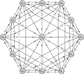
Figure 4: Graph of the transitions caused by the strong arbitrages.

Figure 4 plots the corresponding graph. Figure 5 plots a similar graph, where the numbers of the arbitrages from Table 1 are included, instead of the numbers of strong arbitrages.

Proof.

By inspection follows from Proposition 16. ∎

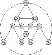
Figure 6: The polyhedral representation of the principal graph.

Ignoring the zero vertex $\mathscr{D}_{0}$, the edges that lead to this vertex and directions of the edges, another, polyhedral, representation of the graph plotted in Fig. 4 is given in Fig. 6. The corresponding polyhedron is a distorted triangular orthobicupola, shown in Fig. 1. The incidence matrix $I$ of the graph plotted in Fig. 6 is as follows:

$$I=\left(\hbox{}\,\vbox{\Let@\restore@math@cr\default@tag\halign{\hfill$\m@th\scriptstyle#$\hfil&&\space\hfill$\m@th\scriptstyle#$\hfil\cr 1& \hfill$\scriptstyle 1& \hfill$\scriptstyle 0& \hfill$\scriptstyle 0& \hfill$\scriptstyle 1& \hfill$\scriptstyle 0& \hfill$\scriptstyle 0& \hfill$\scriptstyle 0& \hfill$\scriptstyle 1& \hfill$\scriptstyle 0& \hfill$\scriptstyle 0& \hfill$\scriptstyle 1\\ 1& \hfill$\scriptstyle 1& \hfill$\scriptstyle 1& \hfill$\scriptstyle 1& \hfill$\scriptstyle 0& \hfill$\scriptstyle 0& \hfill$\scriptstyle 0& \hfill$\scriptstyle 0& \hfill$\scriptstyle 0& \hfill$\scriptstyle 0& \hfill$\scriptstyle 0& \hfill$\scriptstyle 1\\ 0& \hfill$\scriptstyle 1& \hfill$\scriptstyle 1& \hfill$\scriptstyle 1& \hfill$\scriptstyle 0& \hfill$\scriptstyle 0& \hfill$\scriptstyle 1& \hfill$\scriptstyle 0& \hfill$\scriptstyle 0& \hfill$\scriptstyle 0& \hfill$\scriptstyle 1& \hfill$\scriptstyle 0\\ 0& \hfill$\scriptstyle 1& \hfill$\scriptstyle 1& \hfill$\scriptstyle 1& \hfill$\scriptstyle 1& \hfill$\scriptstyle 1& \hfill$\scriptstyle 0& \hfill$\scriptstyle 0& \hfill$\scriptstyle 0& \hfill$\scriptstyle 0& \hfill$\scriptstyle 0& \hfill$\scriptstyle 0\\ 1& \hfill$\scriptstyle 0& \hfill$\scriptstyle 0& \hfill$\scriptstyle 1& \hfill$\scriptstyle 1& \hfill$\scriptstyle 1& \hfill$\scriptstyle 0& \hfill$\scriptstyle 0& \hfill$\scriptstyle 1& \hfill$\scriptstyle 0& \hfill$\scriptstyle 0& \hfill$\scriptstyle 0\\ 0& \hfill$\scriptstyle 0& \hfill$\scriptstyle 0& \hfill$\scriptstyle 1& \hfill$\scriptstyle 1& \hfill$\scriptstyle 1& \hfill$\scriptstyle 1& \hfill$\scriptstyle 1& \hfill$\scriptstyle 0& \hfill$\scriptstyle 0& \hfill$\scriptstyle 0& \hfill$\scriptstyle 0\\ 0& \hfill$\scriptstyle 0& \hfill$\scriptstyle 1& \hfill$\scriptstyle 0& \hfill$\scriptstyle 0& \hfill$\scriptstyle 1& \hfill$\scriptstyle 1& \hfill$\scriptstyle 1& \hfill$\scriptstyle 0& \hfill$\scriptstyle 0& \hfill$\scriptstyle 1& \hfill$\scriptstyle 0\\ 0& \hfill$\scriptstyle 0& \hfill$\scriptstyle 0& \hfill$\scriptstyle 0& \hfill$\scriptstyle 0& \hfill$\scriptstyle 1& \hfill$\scriptstyle 1& \hfill$\scriptstyle 1& \hfill$\scriptstyle 1& \hfill$\scriptstyle 1& \hfill$\scriptstyle 0& \hfill$\scriptstyle 0\\ 1& \hfill$\scriptstyle 0& \hfill$\scriptstyle 0& \hfill$\scriptstyle 0& \hfill$\scriptstyle 1& \hfill$\scriptstyle 0& \hfill$\scriptstyle 0& \hfill$\scriptstyle 1& \hfill$\scriptstyle 1& \hfill$\scriptstyle 1& \hfill$\scriptstyle 0& \hfill$\scriptstyle 0\\ 0& \hfill$\scriptstyle 0& \hfill$\scriptstyle 0& \hfill$\scriptstyle 0& \hfill$\scriptstyle 0& \hfill$\scriptstyle 0& \hfill$\scriptstyle 0& \hfill$\scriptstyle 1& \hfill$\scriptstyle 1& \hfill$\scriptstyle 1& \hfill$\scriptstyle 1& \hfill$\scriptstyle 1\\ 0& \hfill$\scriptstyle 0& \hfill$\scriptstyle 1& \hfill$\scriptstyle 0& \hfill$\scriptstyle 0& \hfill$\scriptstyle 0& \hfill$\scriptstyle 1& \hfill$\scriptstyle 0& \hfill$\scriptstyle 0& \hfill$\scriptstyle 1& \hfill$\scriptstyle 1& \hfill$\scriptstyle 1\\ 1& \hfill$\scriptstyle 1& \hfill$\scriptstyle 0& \hfill$\scriptstyle 0& \hfill$\scriptstyle 0& \hfill$\scriptstyle 0& \hfill$\scriptstyle 0& \hfill$\scriptstyle 0& \hfill$\scriptstyle 0& \hfill$\scriptstyle 1& \hfill$\scriptstyle 1& \hfill$\scriptstyle 1\crcr}}\,\right).$$

Table 3: Transition, caused by strong arbitrages from Table 1

	$\mathscr{D}_{1}$	$\mathscr{D}_{2}$	$\mathscr{D}_{3}$	$\mathscr{D}_{4}$	$\mathscr{D}_{5}$	$\mathscr{D}_{6}$	$\mathscr{D}_{7}$	$\mathscr{D}_{8}$	$\mathscr{D}_{9}$	$\mathscr{D}_{10}$	$\mathscr{D}_{11}$	$\mathscr{D}_{12}$
$\hat{\mathscr{A}}^{(1)}$	$\mathscr{D}_{1}$	$\mathscr{D}_{12}$	$\mathscr{D}_{11}$	$\mathscr{D}_{0}$	$\mathscr{D}_{5}$	$\mathscr{D}_{6}$	$\mathscr{D}_{7}$	$\mathscr{D}_{6}$	$\mathscr{D}_{5}$	$\mathscr{D}_{0}$	$\mathscr{D}_{11}$	$\mathscr{D}_{12}$
$\hat{\mathscr{A}}^{(2)}$	$\mathscr{D}_{1}$	$\mathscr{D}_{2}$	$\mathscr{D}_{3}$	$\mathscr{D}_{0}$	$\mathscr{D}_{9}$	$\mathscr{D}_{8}$	$\mathscr{D}_{7}$	$\mathscr{D}_{8}$	$\mathscr{D}_{9}$	$\mathscr{D}_{0}$	$\mathscr{D}_{3}$	$\mathscr{D}_{2}$
$\hat{\mathscr{A}}^{(3)}$	$\mathscr{D}_{1}$	$\mathscr{D}_{0}$	$\mathscr{D}_{7}$	$\mathscr{D}_{6}$	$\mathscr{D}_{5}$	$\mathscr{D}_{6}$	$\mathscr{D}_{7}$	$\mathscr{D}_{0}$	$\mathscr{D}_{1}$	$\mathscr{D}_{12}$	$\mathscr{D}_{11}$	$\mathscr{D}_{12}$
$\hat{\mathscr{A}}^{(4)}$	$\mathscr{D}_{1}$	$\mathscr{D}_{0}$	$\mathscr{D}_{3}$	$\mathscr{D}_{4}$	$\mathscr{D}_{5}$	$\mathscr{D}_{4}$	$\mathscr{D}_{3}$	$\mathscr{D}_{0}$	$\mathscr{D}_{9}$	$\mathscr{D}_{10}$	$\mathscr{D}_{11}$	$\mathscr{D}_{10}$
$\hat{\mathscr{A}}^{(5)}$	$\mathscr{D}_{1}$	$\mathscr{D}_{2}$	$\mathscr{D}_{3}$	$\mathscr{D}_{2}$	$\mathscr{D}_{1}$	$\mathscr{D}_{0}$	$\mathscr{D}_{7}$	$\mathscr{D}_{8}$	$\mathscr{D}_{9}$	$\mathscr{D}_{8}$	$\mathscr{D}_{7}$	$\mathscr{D}_{0}$
$\hat{\mathscr{A}}^{(6)}$	$\mathscr{D}_{5}$	$\mathscr{D}_{4}$	$\mathscr{D}_{3}$	$\mathscr{D}_{4}$	$\mathscr{D}_{5}$	$\mathscr{D}_{0}$	$\mathscr{D}_{11}$	$\mathscr{D}_{10}$	$\mathscr{D}_{9}$	$\mathscr{D}_{10}$	$\mathscr{D}_{11}$	$\mathscr{D}_{0}$
$\hat{\mathscr{A}}^{(7)}$	$\mathscr{D}_{1}$	$\mathscr{D}_{1}$	$\mathscr{D}_{0}$	$\mathscr{D}_{5}$	$\mathscr{D}_{5}$	$\mathscr{D}_{6}$	$\mathscr{D}_{7}$	$\mathscr{D}_{7}$	$\mathscr{D}_{0}$	$\mathscr{D}_{11}$	$\mathscr{D}_{11}$	$\mathscr{D}_{12}$
$\hat{\mathscr{A}}^{(8)}$	$\mathscr{D}_{2}$	$\mathscr{D}_{2}$	$\mathscr{D}_{0}$	$\mathscr{D}_{4}$	$\mathscr{D}_{4}$	$\mathscr{D}_{6}$	$\mathscr{D}_{8}$	$\mathscr{D}_{8}$	$\mathscr{D}_{0}$	$\mathscr{D}_{10}$	$\mathscr{D}_{10}$	$\mathscr{D}_{12}$
$\hat{\mathscr{A}}^{(9)}$	$\mathscr{D}_{1}$	$\mathscr{D}_{2}$	$\mathscr{D}_{3}$	$\mathscr{D}_{3}$	$\mathscr{D}_{0}$	$\mathscr{D}_{7}$	$\mathscr{D}_{7}$	$\mathscr{D}_{8}$	$\mathscr{D}_{9}$	$\mathscr{D}_{9}$	$\mathscr{D}_{0}$	$\mathscr{D}_{1}$
$\hat{\mathscr{A}}^{(10)}$	$\mathscr{D}_{12}$	$\mathscr{D}_{2}$	$\mathscr{D}_{3}$	$\mathscr{D}_{3}$	$\mathscr{D}_{0}$	$\mathscr{D}_{6}$	$\mathscr{D}_{6}$	$\mathscr{D}_{8}$	$\mathscr{D}_{9}$	$\mathscr{D}_{10}$	$\mathscr{D}_{0}$	$\mathscr{D}_{12}$
$\hat{\mathscr{A}}^{(11)}$	$\mathscr{D}_{0}$	$\mathscr{D}_{3}$	$\mathscr{D}_{3}$	$\mathscr{D}_{4}$	$\mathscr{D}_{5}$	$\mathscr{D}_{5}$	$\mathscr{D}_{0}$	$\mathscr{D}_{9}$	$\mathscr{D}_{9}$	$\mathscr{D}_{10}$	$\mathscr{D}_{11}$	$\mathscr{D}_{10}$
$\hat{\mathscr{A}}^{(12)}$	$\mathscr{D}_{0}$	$\mathscr{D}_{2}$	$\mathscr{D}_{2}$	$\mathscr{D}_{4}$	$\mathscr{D}_{6}$	$\mathscr{D}_{6}$	$\mathscr{D}_{0}$	$\mathscr{D}_{8}$	$\mathscr{D}_{8}$	$\mathscr{D}_{10}$	$\mathscr{D}_{12}$	$\mathscr{D}_{12}$

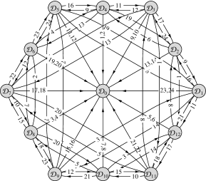
Figure 5: The previous graph with the arbitrage numbers, instead of the strong arbitrage numbers.

Now let us deal with the coupled discrepancies and the incremental dynamics.

Corollary 8.

For any arbitrage chain the corresponding sequence of increments includes only the zero triplet $\mathscr{I}_{0}=(0,0,0)$ or one of the following six triplets:

$$\mathscr{I}_{1} =a(1,\hphantom{-}0,\hphantom{-}0),\quad \mathscr{I}_{2} =a({-}1,\hphantom{-}0,\hphantom{-}0),\quad \mathscr{I}_{3} =a(0,\hphantom{-}1,\hphantom{-}0),$$

$$\mathscr{I}_{4} =a(0,{-}1,\hphantom{-}0),\quad \mathscr{I}_{5} =a(\hphantom{-}0,\hphantom{-}0,\hphantom{-}1),\quad \mathscr{I}_{6} =a(0,\hphantom{-}0,{-}1).$$

The dynamics of the increments $\mathscr{I}$ is conveniently visualised in Fig. 7.

Figure 7: The increment dynamics graph

The correctness of this description of the dynamics of the increments follows immediately from Corollary 7 and Proposition 18. The legitimacy of the algorithms relevant to Theorem 1 and, therefore, proof of Theorem 1 and Proposition 8 follows from Figs. 5 and 7.

We note also that the 24-periodic chain of arbitrage from Proposition 6 was also found looking at Fig. 5 and 7. The corresponding route is quite natural from this perspective, and is given by

$$\mathscr{D}_{10} \to ~{}\mathscr{D}_{11} \to ~{}\mathscr{D}_{10} \to ~{}\mathscr{D}_{12} \to ~{}\mathscr{D}_{1} \to ~{}\mathscr{D}_{12} \to ~{}\mathscr{D}_{2} \to ~{}\mathscr{D}_{3} \to$$ (31)

$$\mathscr{D}_{2} \to \mathscr{D}_{4} \to \mathscr{D}_{5} \to \mathscr{D}_{4} \to \mathscr{D}_{6} \to \mathscr{D}_{7} \to \mathscr{D}_{6} \to \mathscr{D}_{8} \to$$

$$\mathscr{D}_{9} \to \mathscr{D}_{8} \to \mathscr{D}_{10} \to \mathscr{D}_{8} \to \mathscr{D}_{6} \to \mathscr{D}_{4} \to \mathscr{D}_{2} \to ~{}\mathscr{D}_{12} \to ~{}\mathscr{D}_{10}.$$

9.7 Commuters, Terminals and Knots

Now we move to a proof of Theorem 2 and Proposition 11. The case $d_{\textrm{€}\textrm{\pounds}}=d_{\textrm{€}\textrm{\yen}}$ has been considered in Section 8.1. Thus we can assume that $d_{\textrm{€}\textrm{\pounds}}\not=d_{\textrm{€}\textrm{\yen}}$.

The focus is again on the dynamics of the exchange rate discrepancies. The set of all discrepancies that may be achievable from $\mathscr{D}=(a,b,0)$ contains altogether 61 different elements, see Corollary 7. The corresponding connected component ${\boldsymbol{D}}(a,b)$, which contains $\mathscr{D}=(a,b,0)$, see (29), contains 24 elements listed in (29). To describe the detailed structure of this set we will introduce a new notation. The set ${\boldsymbol{D}}(a,b)$, contains six elements that have all three components that are non-zero, and we re-denote these elements by

$$C_{1} =\left(a,b,-a+b\right), C_{2} =\left(-a+b,b,a\right), C_{3} =\left(a,a-b,-b\right),$$

$$C_{4} =\left(-a+b,-a,-b\right),\quad C_{5} =\left(-b,a-b,a\right),\quad C_{6} =\left(-b,-a,-a+b\right).$$

We call these ensembles commuters by way of analogy with passenger travel.

We call an element with two non-zero components a terminal, if $d_{1}\not=\pm d_{2}$. There are altogether 18 terminals in ${\boldsymbol{D}}(a,b)$. To each commuter $C_{i}$, $i=1,\ldots,6$, we relate three terminals $T^{j}_{i}$, $j=1,2,3$, as follows:

$$T^{1}_{1} =\left(0,b,-a+b\right), T^{2}_{1} =\left(a,0,-a+b\right), T^{3}_{1} =\left(a,b,0\right);$$

$$T^{1}_{2} =\left(0,b,a\right), T^{2}_{2} =\left(-a+b,0,a\right), T^{3}_{2} =\left(-a+b,b,0\right);$$

$$T^{1}_{3} =\left(0,-a,-b\right), T^{2}_{3} =\left(-a+b,0,-b\right), T^{3}_{3} =\left(-a+b,-a,0\right);$$

$$T^{1}_{4} =\left(0,a-b,-b\right), T^{2}_{4} =\left(a,0,-b\right), T^{3}_{4} =\left(a,a-b,0\right);$$

$$T^{1}_{5} =\left(0,a-b,a\right), T^{2}_{5} =\left(-b,0,a\right), T^{3}_{5} =\left(-b,a-b,0\right);$$

$$T^{1}_{6} =\left(0,-a,-a+b\right),\quad T^{2}_{6} =\left(-b,0,-a+b\right),\quad T^{3}_{6} =\left(-b,-a,0\right).$$

Lemma 8.

The equalities

$$C_{i}G^{(7)} =T^{1}_{i}, \quad C_{i}H^{(7)} =(0,0,0),$$

$$C_{i}G^{(9)} =T^{2}_{i}, \quad C_{i}H^{(9)} =(0,0,0),$$

$$C_{i}G^{(11)} =T^{3}_{i}, \quad C_{i}H^{(11)} =(0,0,0)$$

hold for $i=1,\ldots,6$. Also the following equalities hold: $T^{j}_{i}G^{(k)}=C_{i}$, for $i=1,\ldots,6$, $j=1,2,3$, $k=8,10,12$.

We group the commuters and terminals in six knots, $K_{1},\ldots,K_{6}$ as follows:

$$K_{i}=\left\{C_{i},T^{1}_{i},T^{2}_{i},T^{3}_{i}\right\},\quad i=1,\ldots,6.$$

Figure 8 illustrates behaviour at a knot.

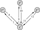
Figure 8: The “commuter–terminals” graph of a knot

9.8 Travel Between Knots

Departing from a particular terminal, and applying some arbitrages with numbers $k=7,\ldots,12$, one can travel to another terminal belonging to a different knot, simultaneously “loading some cargo” upon the corresponded triplet $\mathscr{R}^{\prime}$. Details are given in the following proposition.

Proposition 19.

The following groups of equalities hold:

$$\left\{\begin{aligned} T^{1}_{1}G^{(3)}&=T^{1}_{2},\quad&T^{1}_{1}H^{(3)}&=(0,a,0),\quad&T^{1}_{1}G^{(5)}&=T^{2}_{4},\quad&T^{1}_{1}H^{(5)}&=(0,0,b);\\ T^{2}_{1}G^{(1)}&=T^{1}_{6},\quad&T^{2}_{1}H^{(1)}&=(-a,0,0),\quad&T^{2}_{1}G^{(6)}&=T^{3}_{3},\quad&T^{2}_{1}H^{(6)}&=(0,0,-a);\\ T^{3}_{1}G^{(2)}&=T^{2}_{6},\quad&T^{3}_{1}H^{(2)}&=(-b,0,0),\quad&T^{3}_{1}G^{(4)}&=T^{3}_{2},\quad&T^{3}_{1}H^{(4)}&=(0,a-b,0);\end{aligned}\right.\\$$

$$\left\{\begin{aligned} T^{1}_{2}G^{(2)}&=T^{2}_{5},\quad&T^{1}_{2}H^{(2)}&=(-b,0,0),\quad&T^{1}_{2}G^{(4)}&=T^{3}_{1},\quad&T^{1}_{2}H^{(4)}&=(0,-a,0);\\ T^{3}_{2}G^{(1)}&=T^{2}_{2},\quad&T^{3}_{2}H^{(1)}&=(a-b,0,0),\quad&T^{3}_{2}G^{(6)}&=T^{3}_{3},\quad&T^{3}_{2}H^{(6)}&=(0,0,-a);\end{aligned}\right.\\$$

$$\left\{\begin{aligned} T^{1}_{3}G^{(2)}&=T^{2}_{4},\quad&T^{1}_{3}H^{(2)}=(a,0,0),\quad&T^{1}_{3}G^{(4)}&=T^{3}_{6},\quad&T^{2}_{3}H^{(4)}=(0,b,0);\end{aligned}\right.\\$$

$$\left\{\begin{aligned} T^{1}_{4}G^{(2)}&=T^{2}_{3},\quad&T^{1}_{4}H^{(2)}&=(-a+b,0,0),\quad&T^{1}_{4}G^{(4)}&=T^{3}_{5},\quad&T^{1}_{4}H^{(4)}&=(0,b,0);\\ T^{3}_{4}G^{(1)}&=T^{1}_{3},\quad&T^{3}_{4}H^{(1)}&=(-a,0,0),\quad&T^{3}_{4}G^{(6)}&=T^{3}_{1},\quad&T^{3}_{4}H^{(6)}&=(0,0,-b);\end{aligned}\right.\\$$

$$\left\{\begin{aligned} T^{1}_{5}G^{(2)}&=T^{2}_{2},\quad&T^{1}_{5}H^{(2)}&=(-a+b,0,0),\quad&T^{1}_{5}G^{(4)}&=T^{3}_{4},\quad&T^{1}_{5}H^{(4)}&=(0,-a,0);\\ T^{3}_{5}G^{(1)}&=T^{1}_{2},\quad&T^{3}_{5}H^{(1)}&=(b,0,0),\quad&T^{3}_{5}G^{(6)}&=T^{3}_{6},\quad&T^{3}_{5}H^{(6)}&=(0,0,a);\end{aligned}\right.\\$$

$$\left\{\begin{aligned} T^{1}_{6}G^{(2)}&=T^{2}_{1},\quad&T^{1}_{6}H^{(2)}&=(a,0,0),\quad&T^{1}_{6}G^{(4)}&=T^{3}_{3},\quad&T^{1}_{6}H^{(4)}&=(0,a-b,0).\end{aligned}\right.$$

We introduce the “travel between knots” directed graph $\Gamma$, shown in Fig. 9, as follows. This graph has $6$ vertices that correspond to the knots $K_{1},\ldots,K_{6}$. A knot $K_{i}$ is connected by an arrow with another knot $K_{j}$ if one of terminals belonging to $K^{j}$ figures in the rows belonging to the $i$-th subset of equalities from Proposition 19. For instance, the knot $K_{1}$ is connected with $K_{2},K_{3},K_{4},K_{6}$. Moreover each arrow corresponds to the three dimensional “cargo vector(s)”: these vectors are related in a natural way to the increment vectors in the equalities above. For instance, we attach the cargo-vectors $(0,a-b,0)$ and $(0,a,0)$ to the $K_{1}\to K_{2}$ arrow. The incidence matrix of this graph is written below.

$$I(\Gamma)=\left(\begin{array}[]{cccccc}0&1&0&1&0&1\\ 1&0&1&0&1&0\\ 0&0&0&1&0&1\\ 1&0&1&0&1&0\\ 0&1&0&1&0&1\\ 0&1&0&0&0&0\end{array}\right)$$

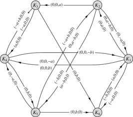
Figure 9: The “travel between knots” graph $\Gamma$

9.9 Finalising the proof of Theorem 2 and Proposition 11

If the single transition $K_{i}\to K_{j}$ is possible we use $W^{i\to j}$ for the corresponding cargo; we will use $W^{i\to j}_{1},W^{i\to j}_{2}$ if two transitions are possible. In the latter case $W^{i\to j}_{1}$ refers to the upper vector indicated at graph $\Gamma$. For instance, $W^{1\to 2}_{1}=(0,a-b,0)$, $W^{1\to 2}_{2}=(0,a,0)$, $W^{2\to 1}=(0,-a,0)$, etc.

Lemma 9.

For any positive integers $N_{1},N_{2},N_{3}$ there exists a chain ${\boldsymbol{\hat{A}}}$ of strong arbitrages such that $\mathscr{R}{\boldsymbol{\hat{A}}}$ has the form

$$(r_{\textrm{\$}\textrm{€}}+m_{1}a-N_{1}b,r_{\textrm{\$}\textrm{\pounds}}+m_{2}a+N_{2}b,r_{\textrm{\$}\textrm{\yen}}+m_{3}a-N_{3}b)$$

where $m_{1},m_{2},m_{3}$ are some positive integer numbers,

Proof.

Since the moves from one terminal to another, within a particular knot, are always possible and do not change $\mathscr{R}^{\prime}$ (see Lemma 8), any route allowed by the graph $\Gamma$ can be performed, and any combination of corresponding cargo can be loaded. For the cycle $K_{1}\to K_{2}\to K_{5}\to K_{6}\to K_{1}$ we have

$$W^{1\to 2}_{1}+W^{2\to 5}_{1}+W^{5\to 6}+W^{6\to 1}=(a-b,a,0).$$

For the cycle $K_{1}\to K_{2}\to K_{3}\to K_{6}\to K_{1}$ we have

$$W^{1\to 2}_{2}+W^{2\to 3}+W^{3\to 6}+W^{6\to 1}=(a,a+b,a).$$

For the cycle $K_{1}\to K_{2}\to K_{3}\to K_{4}\to K_{1}$ we have

$$W^{1\to 2}_{2}+W^{2\to 3}+W^{3\to 4}+W^{4\to 1}=(a,a,a-b).$$

∎

Corollary 9.

For any non-negative integers $N_{1},N_{2},N_{3}$ and $M_{1},M_{2},M_{3}$ there exists a chain ${\boldsymbol{\hat{A}}}$ of strong arbitrages such that $\mathscr{R}{\boldsymbol{\hat{A}}}$ has the form $(r_{\textrm{\$}\textrm{€}}+M_{1}a-N_{1}b,r_{\textrm{\$}\textrm{\pounds}}+M_{2}a+N_{2}b,r_{\textrm{\$}\textrm{\yen}}+M_{3}a-N_{3}b)$.

Proof.

From the lemma above it follows that we can achieve the state

$$(r_{\textrm{\$}\textrm{€}}+m_{1}a-(N_{1}-1)b,r_{\textrm{\$}\textrm{\pounds}}+m_{2}a+(N_{2})b,r_{\textrm{\$}\textrm{\yen}}+m_{3}a-(N_{3}+1)b,a,b,-a+b).$$

Then moving to the terminal $T^{3}_{1}$ and applying arbitrage $\hat{\mathscr{A}}^{(6)}$ we arrive at

$$(r_{\textrm{\$}\textrm{€}}+(m_{1}-1)a-(N_{1})b,r_{\textrm{\$}\textrm{\pounds}}+m_{2}a+(N_{2})b,r_{\textrm{\$}\textrm{\yen}}+m_{3}a-N_{3}b,0,a,0).$$

However, from this state we can, by Proposition 1, adjust the numbers $m_{1},m_{2},m_{3}$ to the targets $M_{1},M_{2},M_{3}$. ∎

Theorem 2 and Proposition 11 follow immediately from this last corollary.

10 Concluding Remarks

The key contribution of this paper is to ask what happens to arbitrage sequences when the number of goods or assets under consideration is four, rather than the two, or occasionally three, usually considered. The model is illustrated with regard to a foreign exchange market with four currencies and traders, so there are $C_{4}^{2}=6$ principal exchange rates. Despite abstracting from various complications – such as transaction costs, capital requirements and risk – that are often invoked to explain the limits to arbitrage, we find that the arbitrage operations conducted by the FX traders can generate periodicity or more complicated behaviour in the ensemble of exchange rates, rather than smooth convergence to a “balanced” ensemble where the law of one price holds.

We use the fiction of an Arbiter, who knows all the actual exchange rates and what a balanced ensemble would be, to bring out the information problem. FX traders tend to specialise in particular currencies, so the assumption that the FX traders are initially aware only of the exchange rates for their own “domestic” currencies is not entirely implausible. We show that the order in which the Arbiter reveals information to individual traders regarding discrepancies in exchange rate ensembles makes a key difference to the arbitrage sequences that will be pursued. The sequences are periodic in nature, and show no clear signs of convergence on a balanced ensemble of exchange rates. The Arbiter might know the law of one price exchange rate ensemble, but the traders have little chance of stumbling onto such an ensemble by way of their arbitrage operations.

The analysis in the present paper raises several issues to pursue in future research. An obvious extension is to allow for a larger number of currencies and ask what happens to the arbitrage sequences as this number becomes large. One interesting modification of the analysis would allow the FX traders to learn that arbitrage sequences tend to be periodic and modify their arbitrage strategies to take the periodicity into account. Another modification would allow some arbitrage operations to be pursued simultaneously, and ask what happens as the limiting case where all arbitrage operations are exploited simultaneously is approached. An alternative reformulation of the analysis would be as a Markov process where the states are sextuples of exchange rates between the four currencies and the passages between the states reflect the effects of arbitrage operations pursued. It would be interesting to see if this could be done without compromising the relative simplicity of the present formulation. Finally, but by no means exhaustively, it would be interesting to work with high frequency data sets to test for the existence of the types of arbitrage sequences postulated in the present paper.

References

- Applegate et al. (2006) Applegate, D. L., Bixby, R. E., Chvátal, V., Cook, W. J., 2006. The traveling salesman problem: A computational study. Princeton Series in Applied Mathematics. Princeton University Press, Princeton, NJ.
- Arrow (1951) Arrow, K. J., 1951. Social Choice and Individual Values. University Press, Yale.
- Asarin et al. (1992) Asarin, E. A., Kozyakin, V. S., Krasnosel′skiĭ, M. A., Kuznetsov, N. A., 1992. Analiz ustoichivosti rassinkhronizovannykh diskretnykh sistem. Nauka, Moscow, in Russian.
- Baddeley (2004) Baddeley, A. D., 2004. Your Memory: a User’s Guide, IVth Edition. Carlton Books, London, UK.
- Bertsekas and Tsitsiklis (1989) Bertsekas, D. P., Tsitsiklis, J. N., 1989. Parallel and Distributed Computation. Numerical Methods. Prentice Hall, Englewood Cliffs. NJ.
- BIS (2010) BIS, 2010. Triennial Central Bank Survey of Foreign Exchange and Derivatives Market Activity in 2010 — Final results. Bank of International Settlement, Basel, Switzerland.
-
Blondel and Tsitsiklis (1997)
Blondel, V. D.,
Tsitsiklis, J. N., 1997. When is a pair of matrices mortal?
Inform. Process. Lett. 63 (5), 283–286.
URL http://dx.doi.org/10.1016/S0020-0190(97)00123-3 -
Blondel and Tsitsiklis (2000a)
Blondel, V. D., Tsitsiklis, J. N., 2000a. The
boundedness of all
products of a pair of matrices is undecidable. Systems Control Lett. 41 (2),
135–140.
URL http://dx.doi.org/10.1016/S0167-6911(00)00049-9 - Blondel and Tsitsiklis (2000b) Blondel, V. D., Tsitsiklis, J. N., 2000b. A survey of computational complexity results in systems and control. Automatica 36 (9), 1249–1274.
- Cassel (1916) Cassel, G., 1916. The present situation of the foreign exchanges. I. Economic Journal 26 (1), 62–65.
-
Covrig and Melvin (2002)
Covrig, V., Melvin, M.,
August 2002. Asymmetric information and price discovery
in the FX market: Does Tokyo know more about the yen? Journal of
Empirical Finance 9 (3), 271–285.
URL http://ideas.repec.org/a/eee/empfin/v9y2002i3p271-285.html - Deardorff (1979) Deardorff, A. V., 1979. One way arbitrage and its implications for the foreign exchange markets. Journal of Political Economy 87 (2), 351–364.
-
D’Souza (2008)
D’Souza, C., 2008. Price discovery
across geographic locations in the foreign
exchange market. Bank of Canada Review Spring 2008, 19–27.
URL http://ideas.repec.org/a/bca/bcarev/v2008y2008ispring08p19-27.html - Dybvig and Ross (2008) Dybvig, P. H., Ross, S. A., 2008. Arbitrage. In: Durlauf, S. N., Blume, L. E. (Eds.), The New Palgrave Dictionary of Economics. Palgrave Macmillan, Basingstoke.
- Engel (1999) Engel, C., 1999. Accounting for us real exchange rate changes. Journal of Political Economy 107 (2), 507–538.
-
Engel and West (2005)
Engel, C., West, K. D., June
2005. Exchange rates and fundamentals. Journal of
Political Economy 113 (3), 485–517.
URL http://ideas.repec.org/a/ucp/jpolec/v113y2005i3p485-517.html -
Evans and Lyons (2008)
Evans, M. D., Lyons, R. K.,
April 2008. How is macro news transmitted to
exchange rates? Journal of Financial Economics 88 (1), 26–50.
URL http://ideas.repec.org/a/eee/jfinec/v88y2008i1p26-50.html - Evans (2011) Evans, M. D. D., 2011. Exchange-Rate Dynamics. Princeton University Press, Princeton, NJ.
-
Evans and Lyons (2002)
Evans, M. D. D., Lyons,
R. K., February 2002. Order flow and exchange rate
dynamics. Journal of Political Economy 110 (1), 170–180.
URL http://ideas.repec.org/a/ucp/jpolec/v110y2002i1p170-180.html -
Evans and Lyons (2005)
Evans, M. D. D., Lyons,
R. K., May 2005. Meese-Rogoff redux: Micro-based
exchange-rate forecasting. American Economic Review 95 (2), 405–414.
URL http://ideas.repec.org/a/aea/aecrev/v95y2005i2p405-414.html -
Fisher (1989)
Fisher, F. M., 1989.
Disequilibrium Foundations of Equilibrium Economics.
Econometric Society Monographs. Cambridge University Press.
URL http://econpapers.repec.org/RePEc:cup:cbooks:9780521378567 -
Froot et al. (2001)
Froot, K. A., Kim, M., Rogoff, K., Nov. 2001. The law of one
price over 700
years. IMF Working Paper WP/01/174, International Monetary Fund, Washington
DC.
URL http://www.imf.org/external/pubs/ft/wp/2001/wp01174.pdf - Galliardo and Heats (2009) Galliardo, P., Heats, A., March 2009. Execution methods in foreigh exchange markets. BIS Quaterly Review, 83–91.
- Garey and Johnson (1979) Garey, M. R., Johnson, D. S., 1979. Computers and intractability: A guide to the theory of NP-completeness. Series of Books in the Mathematical Sciences. W. H. Freeman and Co., San Francisco, Calif.
- Haskel and Wolf (2001) Haskel, J., Wolf, H., 2001. The law of one price: a case study. Scandinavian Journal of Economics 103, 545–558.
- Kaszkurewicz and Bhaya (2000) Kaszkurewicz, E., Bhaya, A., 2000. Matrix diagonal stability in systems and computation. Birkhäuser Boston Inc., Boston, MA.
- Keynes (1923) Keynes, J. M., 1923. A Tract on Monetary Reform. Macmilan, London UK.
- Kozyakin (2004) Kozyakin, V., 2004. A short introduction to asynchronous systems. In: Aulbach, B., Elaydi, S., Ladas, G. (Eds.), Proceedings of the Sixth International Conference on Difference Equations. CRC, Boca Raton, FL, pp. 153–165.
- Kozyakin et al. (2010) Kozyakin, V., O’Callaghan, B., Pokrovskii, A., April 2010. Sequences of arbitrages. ArXiv.org e-Print archive.
- Kozyakin (1990) Kozyakin, V. S., 1990. Algebraic unsolvability of a problem on the absolute stability of desynchronized systems. Avtomat. i Telemekh. (6), 41–47, in Russian, translation in Automat. Remote Control 51 (1990), no. 6, part 1, 754–759.
- Kozyakin (2003) Kozyakin, V. S., 2003. Indefinability in o-minimal structures of finite sets of matrices whose infinite products converge and are bounded or unbounded. Avtomat. i Telemekh. (9), 24–41, in Russian, translation in Autom. Remote Control 64 (2003), no. 9, 1386–1400.
- Kozyakin (2003) Kozyakin, V. S., May 2003. Asynchronous systems: A short survey and problems. Preprint 13/2003, Boole Centre for Research in Informatics, University College Cork — National University of Ireland, Cork.
- Lamont and Thaler (2003) Lamont, O. A., Thaler, R. H., 2003. The law of one price in financial markets. Journal of Economic Perspectives 17 (4), 191–202.
- Lowenstein (2000) Lowenstein, R., 2000. When Genius Failed: the Rise and Fail of Long-Term Capital Management. Random House, New York.
- Lyons (2001) Lyons, R. K., 2001. The Microstructure Approach to Exchange Rates. MIT Press, Cambridge, MA.
-
Marshall et al. (2007)
Marshall, B. R., Treepongkaruna, S., Young, M.,
2007. Exploitable arbitrage
opportunities exist in the foreign exchange market. Discussion Paper, 10
September, Massey University, Palmerston North, New Zealand.
URL http://wwwdocs.fce.unsw.edu.au/banking/seminar/2007/exploitablearbitrage_Marshall_Sept13.pdf -
Meese and Rogoff (1983)
Meese, R. A., Rogoff, K.,
February 1983. Empirical exchange rate models of the
seventies: Do they fit out of sample? Journal of International Economics
14 (1-2), 3–24.
URL http://ideas.repec.org/a/eee/inecon/v14y1983i1-2p3-24.html - Obstfeld and Rogoff (2001) Obstfeld, M., Rogoff, K., 2001. The Six Major Puzzles in International Financies: Is there a Common Cause? MIT Press, Cambridge MA, pp. 339–390.
-
Osler (2005)
Osler, C. L., March 2005. Stop-loss
orders and price cascades in currency
markets. Journal of International Money and Finance 24 (2), 219–241.
URL http://ideas.repec.org/a/eee/jimfin/v24y2005i2p219-241.html -
Rahi and Zigrand (2008)
Rahi, R., Zigrand, J.-P.,
2008. Arbitrage networks. London School of Economics
and Political Science, London, UK.
URL http://vishnu.lse.ac.uk/Rohit_Rahi/Homepage_files/nwtworks.pdf - Rogers (2001) Rogers, J., 2001. Price Level Convergence, Relative Prices and Inflation in Europe. No. 699 in International Finance Discussion Paper. Princeton, New Jersey.
- Rogoff (1996) Rogoff, K., 1996. The purchasing power parity puzzle. Journal of Economic Literature 34 (2), 647–668.
- Ross (1978) Ross, S. A., 1978. A simple approach to the valuation of risky streams. Journal of Business 51, 453–475.
- Sarno and Taylor (2001) Sarno, L., Taylor, M. P., 2001. Microstructure of the Foreign-Exchange Market: a Selective Survey of the Literature. No. 89 in Princeton Studies in International Economics. Princeton University.
- Shleifer and Vishny (1997) Shleifer, A., Vishny, R. W., 1997. The limits of arbitrage. Journal of Finance 52 (1), 35–55.
- Taylor (2002) Taylor, A., 2002. A century of purchasing power parity. Review of Economics and Statistics 84, 139–150.
-
Tsitsiklis and Blondel (1997)
Tsitsiklis,
J. N., Blondel, V. D., 1997. Lyapunov exponents of pairs of
matrices. A correction: “The Lyapunov exponent and joint spectral
radius of pairs of matrices are hard—when not impossible—to compute and
to approximate”. Math. Control Signals Systems 10 (4), 381.
URL http://dx.doi.org/10.1007/BF01211553 - Wolf (2003) Wolf, H., 2003. Annex D: International Relative Prices: Facts and Interpretation. H.M. Treasury, London, UK, pp. 53–73.