Different types of the dimensional crossover in the quasi-one-dimensional spinless fermion systems

Abstract

It is known that many-body correlations qualitatively modify the properties of a one-dimensional metal. However, for a quasi-one-dimensional metal these correlations are suppressed, at least partially. We study conditions under which the one-dimensional effects significantly influence the dimensional crossover of a quasi-one-dimensional metal. It is proved (i) that even a system with very high anisotropy of the single-particle hopping might behave on both sides of the crossover as an ordinary weakly non-ideal Fermi gas. Further, (ii) to demonstrate well-developed signatures of one-dimensional correlations the system must have extremely (exponentially) high anisotropy. Between cases (i) and (ii) an intermediate regime lies: (iii) the one-dimensional phenomena affect the two-particle susceptibilities, but do not reveal themselves in single-particle quantities. Unlike the normal state properties, (iv) the ordering transition is always very sensitive to the anisotropy: the mean field theory quickly becomes invalid as the anisotropy increases. An expression for the transition temperature is derived. The attributes (i-iv) are used to classify the weakly interacting quasi-one-dimensional fermion systems.

I Introduction

Several physical systems may be viewed as quasi-one-dimensional (Q1D) fermionic liquids. These include materials with the Q1D anisotropy of the electron hopping(e.g., Bechgaard salts, blue bronzes Grüner (2000)), cold atoms in an anisotropic trap Moritz et al. (2005), and the artificially created atomic lattices Crain and Himpsel (2006).

The most universal feature of the Q1D systems is the dimensional crossover (DC): at the temperatures exceeding some characteristic scale $T_{x}$ a system behaves as an array of almost independent one-dimensional (1D) units, while below $T_{x}$ a genuine 3D behavior is recovered. The description of this crossover is of fundamental importance for the theory of the systems in question.

Theoretically, the Q1D systems are frequently pictured as a lattice of 1D chains, each chain is represented by a 1D Tomonaga-Luttinger model Gogolin et al. (1998), and closely located chains are coupled by the weak transverse single-electron hopping, or the weak interchain interaction, or both. It is often assumed that the DC occurs between the Tomonaga-Luttinger liquid at high energy and the three-dimensional (3D) Fermi liquid at low energy. Since the Tomonaga-Luttinger excitations are usually represented in terms of the bosonic quantum numbers (however, see Refs. Mattis and Lieb (1965); Rozhkov (2005, 2006, 2008); Imambekov and Glazman (2009)), one has to describe how the 1D bosons cross over to the 3D fermions. This is, of course, a difficult task.

A diverse set of the many-body tools has been used to study the DC. Analytical renormalization group (RG) is applied in Refs. Prigodin and Firsov (1979); Bourbonnais and Caron (1986); Bourbonnais and Caron (1988). Numerical RG is employed in Refs. Duprat and Bourbonnais (2001); Nickel et al. (2005); Fuseya and Ogata (2007); Fuseya et al. (2007). Modification of the dynamical mean field theory to the Q1D fermions is used in Ref. Biermann et al. (2001). Variational technique which explicitly construct both high-energy boson excitations and low-energy fermion excitations is proposed in Refs. Rozhkov (2003, 2009a). Different versions of the random phase approximations (RPA) are also used, Refs. Aizawa et al. (2009); Tanaka and Kuroki (2004).

However, the Tomonaga-Luttinger-liquid-based approaches to the crossover may, in some situations, overcomplicate the theory. It is important to realize that the DC, by itself, is not a many-body phenomenon. Instead, its origin is purely kinematic: it occurs when the temperature becomes comparable to the transverse electron hopping. As such, it occurs even for systems with no interaction Bourbonnais et al. (2003, 2002). Thus, the presence of the crossover does not immediately imply that the the high-energy phase is fundamentally different from the low-energy phase.

The free Q1D system is, of course, a trivial example. However, it may be generalized to a less obvious case of the weakly interacting system. Specifically, we will prove in this paper that in a broad parameter region the Q1D fermions on both sides of the DC are closer to the weakly non-ideal Fermi gas than to a collection of the Tomonaga-Luttinger liquids. Further, we demonstrate that, as parameters are varied, the DC itself experiences several crossovers. It evolves from Fermi-liquid-to-Fermi-liquid type at low anisotropy and interaction to Tomonaga-Luttinger-liquid-to-Fermi-liquid at high anisotropy and interaction, with a more exotic possibility in between.

These different types of the DC may be characterized in terms of the applicability of the low-order perturbation theory. The crossover between the Tomonaga-Luttinger and the Fermi liquid may not be described by the perturbation theory. One can deduce that from the fact that the Tomonaga-Luttinger state is non-perturbative. As the anisotropy or interaction decreases, the applicability of the perturbation theory improves: below certain limit, the perturbation theory can be used for the single-particle properties, but not for the two-particle properties. When even the two-particle properties are within the range of the perturbation theory, the Q1D fermions behave as a Fermi liquid both at high and low energies. Note that such conductor may have very high anisotropy.

Finally, we investigate the applicability of the mean field theory for the Q1D fermions. Apparently, if the anisotropy is large an ordering transition is not of the mean field character. However, one expects that below a certain point the mean field theory becomes accurate. It is surprising to discover that even for a system whose normal state is well-described by the perturbation theory the mean field theory may fail. We will prove that the mean field theory works only if the hopping anisotropy is of the order of unity Rozhkov (2009b).

The paper is organized as follows. In Sec. II the model under study is described. We derive the condition which guarantees the validity of the perturbation theory for the single-particle properties in Sec. III. In Sec. IV similar condition for the two-particle properties is established. In Sec. V the applicability of the mean field theory is discussed. The results of these sections are used in Sec. VI to introduce a classification of the anisotropic Fermi liquids. The results are discussed in Sec. VII. Sec. VIII is reserved for the conclusions.

II Model

We study the following system of the interacting spinless fermions:

$$H=\sum_{i}\int_{0}^{L}dx{\cal H}_{i}^{\rm 1d}+\sum_{i,j}\int_{0}^{L}dx{\cal H}_{ij}^{\perp},$$ (4)

$${\cal H}_{i}^{\rm 1d}={\rm i}v_{\rm F}\left(\colon\psi^{\dagger}_{{\rm L}i}\nabla\psi^{\vphantom{\dagger}}_{{\rm L}i}\colon-\colon\psi^{\dagger}_{{\rm R}i}\nabla\psi^{\vphantom{\dagger}}_{{\rm R}i}\colon\right)+g\rho_{\rm R}\rho_{\rm L},$$

$${\cal H}_{ij}^{\perp}=-t(i-j)\sum_{p={\rm L,R}}\psi^{\dagger}_{pi}\psi^{\vphantom{\dagger}}_{pj}+{\rm h.c.},$$

$$\rho_{pi}=\colon\psi^{\dagger}_{pi}\psi^{\vphantom{\dagger}}_{pi}\colon,$$

where the fermionic field $\psi_{pi}^{\dagger}$ creates a physical fermion with the chirality $p={\rm L}$ or $p={\rm R}$ on chain $i$. The chains are parallel to each other and form a 1D or 2D square lattice in the directions transverse to the chains. Colons stand for the normal ordering. The microscopic cutoff of the model is denoted by $\Lambda$. The transverse tunneling amplitudes $t(i-j)$ depend on the distance $|i-j|$ between the chains. If $t=0$ our Hamiltonian corresponds to a number of decoupled Tomonaga-Luttinger systems. Below we will assume that $t(i-j)$ is non-zero for the nearest neighbors only. Generalization beyond this assumption does not bring new features to the discussion.

The dimensionless interaction parameter is required to be small:

$$\tilde{g}=\frac{g}{2\pi v_{\rm F}}\ll 1.$$ (5)

Here $g$ is the bare interaction strength, and $v_{\rm F}$ is the Fermi velocity.

In principle, the transverse interactions can be also considered. Sufficiently strong transverse interactions may trigger symmetry-breaking phase transition at the temperature exceeding the single-particle DC. We do not want to study this regime, and assume that the transverse interactions are zero.

III Perturbation theory for single-particle properties

III.1 General remarks on the perturbation theory for the Q1D systems

For a generic Fermi system the smallness of the interaction constant is a sufficient condition for the applicability of the perturbation theory. While the perturbative expansion contains divergent terms (e.g., the Cooper diagram grows logarithmically for $T\rightarrow 0$), these divergences are well-understood, and the recipes for the perturbative calculations of the physically relevant quantities are known.

Unfortunately, this program cannot be directly adopted for a Q1D Fermi system: some perturbation theory terms, while small for a generic Fermi liquid, in a Q1D case may be finite, but parametrically large. This phenomenon occurs because the pure 1D fermion system has additional divergent diagrams which are finite for the higher-dimensional Fermi liquid. In Q1D system, the latter divergences are capped by arbitrary weak transverse hopping, yet, the diagram values are affected by the proximity to the divergences. Applying blindly the usual schemes in such a situation may lead to significant qualitative errors in the estimation of the effective parameters of the system. We will study below what limitations should be placed on the microscopic constants of our model to guarantee that these diagrams remain small, and the generic perturbation theory procedures may be implemented.

In addition to the purely mathematical, formal side, the perturbation theory applicability criteria carry important physical information about the DC. When the system experience the crossover from the Tomonaga-Luttinger liquid at high energy to the Fermi liquid at low energy, the perturbation theory is useless due to non-perturbative nature of the Tomonaga-Luttinger liquid. On the other hand, if the perturbation theory is applicable, the system behaves as a Fermi liquid even above the crossover. An accurate analysis reveals that a more exotic possibility is also possible. With this considerations in mind we start our study of the perturbation theory for the Q1D fermions.

III.2 Diagram evaluation approach

If we were to use the perturbation theory in order of $\tilde{g}$ to study Hamiltonian (4), we would discover that, if $t=0$, then several irreducible diagrams are divergent. Three of them are shown in Fig. 1. Others can be constructed from these by inverting the chirality labels or directions of the arrows on the fermion lines.

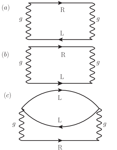
Figure 1: Three divergent diagrams of the 1D metal. Solid lines with arrow and ‘R/L’ chirality labels are fermion propagators. Wiggly lines represent interaction $g$. Panel (a): the “bubble” diagram corresponds to the scattering in the charge-density-wave channel; panel (b): the Cooper diagram describes the scattering in the superconducting channel; panel (c): the single-particle self-energy diagram. Other divergent diagrams can be obtained from (a-c) by inverting the chirality labels or directions of the arrows on the fermion lines.

For example, at $T=0$ the self-energy correction [diagram (c) of Fig. 1] for the electrons of chirality $p$ is equal to

$$\Sigma_{p} = \frac{g^{2}}{16\pi^{2}v_{\rm F}^{2}}(\omega-pv_{\rm F}k+i0)$$

$$\times\ln\left[\frac{v_{\rm F}^{2}k^{2}-(\omega+i0)^{2}}{4v_{\rm F}^{2}\Lambda^{2}}\right]+\ldots,$$

where the ellipsis stands for the non-singular terms, $k$ is the momentum parallel to the chains.

This self-energy contributes to the renormalization of the quasiparticle residue $Z_{p}=1-\delta Z_{p}$:

$$\delta Z_{p}=\frac{g^{2}}{16\pi^{2}v_{\rm F}^{2}}\ln\left|\frac{4v_{\rm F}^{2}\Lambda^{2}}{v_{\rm F}^{2}k^{2}-\omega^{2}}\right|+\ldots$$ (7)

The logarithmic divergence of $\delta Z_{p}$ on the mass surface implies the breakdown of the Landau theory of the Fermi liquid for 1D Fermi systems.

For Q1D system Eq. (7) is not applicable near the mass surface. Indeed, the divergence of the self-energy is purely 1D effect Maslov (2005). Therefore, the growth of $\delta Z_{p}$ at small energy and momenta is cut off at the scale $\sim t$:

$$\delta Z_{p}(\omega,k,{\bf k}_{\perp})<\delta Z_{p}^{\rm max}\approx\frac{g^{2}}{8\pi^{2}v_{\rm F}^{2}}\ln\left(\frac{v_{\rm F}\Lambda}{t}\right).$$ (8)

A detailed derivation of this result is given in Ref. Rozhkov, 2003.

Equation (8) can be used to determine the applicability limits of the perturbation theory: the expansion in orders of $\tilde{g}$ is valid if

$$\delta Z_{p}^{\rm max}\ll 1\Leftrightarrow t\gg t^{\rm 1P},$$ (9)

$$t^{\rm 1P}=v_{\rm F}\Lambda\exp\left(-\frac{2}{\tilde{g}^{2}}\right).$$ (10)

Thus, if the transverse tunneling exceeds the exponentially small value $t^{\rm 1P}$, the self-energy diagram is not only finite, but also small. Smallness of $\delta Z_{p}$ implies that the perturbatively defined fermionic quasiparticles are “good” excitations of our system both above and below the crossover.

Our calculations, however, do not evaluate higher-order contributions to $Z$. They can be easily found with the help of a different approach, which will be presented in the next subsection.

III.3 Renormalization group argument

The applicability of the perturbation theory may be discussed using different type of reasoning. Specifically, consider the renormalization-group (RG) flow near the Tomonaga-Luttinger fixed point. When the cutoff is reduced from $\Lambda$ to $\tilde{\Lambda}$, the effective value of $t$ becomes

$$\tilde{t}_{\tilde{\Lambda}}=t\left(\frac{\tilde{\Lambda}}{\Lambda}\right)^{\theta},$$ (11)

where $\theta\approx\tilde{g}^{2}/2$ is the anomalous dimension of the hopping operator. This RG scaling is applicable until $v_{\rm F}\tilde{\Lambda}\propto\tilde{t}_{\tilde{\Lambda}}$, at which point

$$\tilde{t}=t\left(\frac{t}{v_{\rm F}\Lambda}\right)^{\frac{\theta}{1-\theta}}=t\exp\left[{\frac{\theta}{1-\theta}}\log\left(\frac{t}{v_{\rm F}\Lambda}\right)\right].$$ (12)

This formula may be used to evaluate the DC scale: $T_{x}\propto\tilde{t}$. At energies below $T_{x}$ one cannot view the system as 1D even approximately. Rather, it behaves as the anisotropic multidimensional (2D or 3D) Fermi liquid with the effective hopping $\tilde{t}$ and cutoff $\tilde{\Lambda}$.

At small $\theta$ one can attempt to expand the exponent in Eq. (12):

$$\tilde{t}=t\left[1+\left({\frac{\theta}{1-\theta}}\right)\ln\left(\frac{t}{v_{\rm F}\Lambda}\right)+\ldots\right].$$ (13)

When condition Eq. (9) is satisfied, this expansion is valid, and the renormalization of the transverse hopping is small. Otherwise, $t$ experiences strong renormalization which cannot be captured by Eq. (13), and full Eq. (12) must be used.

To establish the connection with the discussion of the previous subsection, observe that the effective hopping may be written as

$$\tilde{t}=tZ_{p}=t+\delta Z_{p}t.$$ (14)

Therefore, the expression in the square brackets in Eq. (13) is nothing but the expansion of $Z_{p}$ in orders of $\theta=O(\tilde{g}^{2})$ whose lowest order term is given by Eq. (8).

The main advantage of the presented argument is that it automatically accounts for the higher-order contributions: one can keep as many terms in the expansion Eq. (13) as needed. Furthermore, this approach makes the statement of this section almost arithmetical: in order to measure reliably the exponent $\alpha$ of a power-law function $f(x)=x^{\alpha}$ one must sample the function $f$ over an exponentially large range of $x$. For example, the transverse conductivity $\sigma_{y}$ at $v_{\rm F}\Lambda>T>T_{x}$ demonstrates the non-universal power-law behavior Lopatin et al. (2001):

$$\sigma_{y}\propto\left(\frac{T}{v_{\rm F}\Lambda}\right)^{-1+2\theta}.$$ (15)

However, this non-universality may be detected only if the ratio $(T_{x}/v_{\rm F}\Lambda)$ is exponentially large. Otherwise, Eq. (15) is indistinguishable from (see Eq. (71) of Ref. Lopatin et al. (2001))

$$\sigma_{y}\propto 1/(g^{2}T)$$ (16)

with weak corrections. Equation (16) contains only universal exponents. Thus, on experiment the universal transverse transport indicates the validity of Eq. (9) and the applicability of the perturbation theory for the single-particle propagator.

IV Perturbation theory for two-particle properties

IV.1 Diagram evaluation approach

The one-dimensional effects affect the two-particle properties as well. Consider the diagrams (a) and (b) in Fig. 1. They contribute to the renormalization of the effective interaction. Diagram (a) represents the scattering of a particle-hole pair, while diagram (b) corresponds to the Cooper pair scattering.

In a generic Fermi liquid diagram (b) has logarithmic divergence when the total momentum of the Cooper pair is zero. For attractive interaction this divergence leads to the Cooper instability. As for diagram (a), it diverges at the nesting vector, provided that the Fermi surface nests well. This diagram is responsible for the density wave instability. For a generic Fermi liquid the channels are said to be decoupled in the sense that the Cooper pair diagram is finite and small in the particle-hole channel, while the particle-hole diagram is finite and small for the Cooper pair scattering.

In 1D systems, however, the channels are coupled: the particle-hole contribution to the Cooper pair scattering is divergent; moreover, the strength of this divergence is equal in magnitude and opposite in sign to the divergence of the Cooper diagram (see Eqs. (1.45) of Ref. Giamarchi (2004)). The same is true about the contribution of the Cooper diagram to the particle-hole channel. This cancellation is a unique 1D feature responsible for the coupling $g$ being exactly marginal.

In Q1D system the contribution of the Cooper diagram to the particle-hole channel and vice versa are finite, but not necessarily small. Let us, for definiteness, consider the particle-hole channel. For the sake of simplicity, assume that the Q1D Fermi surface nests perfectly at the nesting vector ${\bf Q}$. The formal expression for the effective coupling at ${\bf Q}$, to the first order in $\tilde{g}$, is:

$$g_{\rm eff}\approx g\left[1+\frac{g}{2\pi v_{\rm F}}\ln\left(\frac{v_{\rm F}\Lambda}{T}\right)-\frac{g}{2\pi v_{\rm F}}\ln\left(\frac{v_{\rm F}\Lambda}{t}\right)\right].$$ (17)

The first term here is the bare coupling, the second term corresponds to the “bubble” diagram correction, and the third term is the contribution of the Cooper diagram for $T\ll t$. Both corrections are small provided that

$$t\gg t^{\rm 2P},$$ (18)

$$T\gg t^{\rm 2P},$$ (19)

$$t^{\rm 2P}=v_{\rm F}\Lambda\exp\left(-\frac{2\pi v_{\rm F}}{g}\right)=v_{\rm F}\Lambda\exp\left(-\frac{1}{\tilde{g}}\right).$$ (20)

If we were to consider the effective interaction in the Cooper channel, we would, going through the same steps, obtain the same result.

Eqs. (18) and (19) define the parameter region in which the susceptibility may be calculated perturbatively. Equation (18) ensures the destruction of the non-perturbative 1D effects. Equation (19) must be enforced for a reason which has nothing to do with 1D phenomena: below $t^{\rm 2P}$ the non-perturbative physics of the approaching phase transition starts to affect the susceptibility.

IV.2 Renormalization group argument

It is instructive to rederive Eq. (18) in a fashion similar to the one presented in subsection III.3. To this end, consider the charge-density wave (CDW) susceptibility $\chi_{\rm CDW}$ for $T>T_{x}$ (see, e.g., Eq. (1.68) of Ref. Giamarchi (2004)):

$$\chi_{\rm CDW}(T)=\frac{1}{2\pi v_{\rm F}\tilde{g}}\left[1-\left(\frac{v_{\rm F}\Lambda}{T}\right)^{2\tilde{g}}\right]+\ldots,$$ (21)

where the ellipsis stands for non-singular contributions to the susceptibility. Thus, the expansion in powers of $g$

$$\chi_{\rm CDW}=-\frac{1}{\pi v_{\rm F}}\ln\left(\frac{v_{\rm F}\Lambda}{T}\right)-\frac{g}{2\pi^{2}v_{\rm F}^{2}}\log^{2}\left(\frac{v_{\rm F}\Lambda}{T}\right)+\ldots,$$ (22)

is valid at $T>T_{x}\sim t$, provided that Eq. (18) is fulfilled.

Therefore, we conclude that, if Eq. (18) holds, the perturbation theory for two-particle quantities is applicable to any order in $g$, and the crossover between the Tomonaga-Luttinger liquid scaling Eq. (21) above $T_{x}$ and the Fermi liquid behavior below $T_{x}$ cannot be observed. To detect the high-energy scaling we must work with with a sufficiently anisotropic, or sufficiently non-ideal system for which Eq. (18) is violated.

V Applicability of the mean field theory

The mean field theory is a valuable tool to study the phase diagrams of interacting systems. Both the mean field theory (e.g., Refs. Parish et al., 2007; Maki et al., 2008; Lebed, 2011, chapter 4.4 of Ref. Ishiguro et al., 1998, chapter 3 of Ref. Grüner, 2000) and the closely-related RPA (e.g., Ref. Tanaka and Kuroki, 2004) have been used in the context of the Q1D fermions. Thus, applicability of the mean field theory is an important issue for a theory of the Q1D Fermi systems.

As we have seen above, the perturbation theory may work well for the Fermi liquids with high anisotropy. The mean field theory, however, is more fragile: we will show that it can be applied only to a system with the anisotropy of the order of unity. In addition, we will derive an expression for the transition temperature which is valid if Eq. (18) is true.

To notice the difficulty facing the mean field theory let us make the following heuristic observation. For an anisotropic system two different formulas for the transition scale can be constructed. The first one is $t^{\rm 2P}$ (for example, the expression of this type is given by Eq. (4.41) of Ref. Ishiguro et al. (1998)) and the second one is

$$T_{\rm CDW}=t\exp\left(-\frac{2\pi v_{\rm F}}{g}\right)=\left(\frac{t}{v_{\rm F}\Lambda}\right)t^{\rm 2P}.$$ (23)

When $t/v_{\rm F}\Lambda\sim 1$ the two answers coincide up to a factor of the order of unity, which is a typical accuracy of the mean field theory (see, e.g., Ref. Kos et al. (2004)). However, if $t/v_{\rm F}\Lambda\ll 1$, then $T_{\rm CDW}\ll t^{\rm 2P}$, and one has to decide which of the two is valid. As it turns out, Eq. (23) is the right answer.

The discussion of the previous paragraph may be cast in a more formal fashion. When inequality (18) holds the third term in Eq. (17) is much smaller than unity and, superficially, can be neglected.

Once it is neglected the geometrical progression of the divergent “bubble” diagrams contributing to $g_{\rm eff}$ must be summed. If $g>0$ the coupling $g_{\rm eff}$ found in such a manner diverges at $T=t^{\rm 2P}$, signaling the transition into the CDW state.

This argumentation is invalid, however. The omission of the third term of Eq. (17) on the grounds of its smallness is the offending step. Since the mean field transition temperature is a non-analytical function of the interaction, even a small correction to the latter may lead to large variation of the former.

This property is not unique to the Q1D metallic system. The transition temperature of the Kohn-Luttinger superconductor shows similar sensitivity to the higher-order corrections to the coupling constant (see, e.g., Eq. (31) of Ref. Baranov et al. (2000)).

The correct way to address this issue for a Q1D metal is discussed in Ref. Rozhkov (2009b). Namely, one must perform the RG transformation until the crossover scale $T_{x}$ is reached. No abnormality pertinent to 1D physics is present below $T_{x}$. When the effective Hamiltonian at the crossover scale is found, the mean field calculations can be safely applied to it, and Eq. (23) is recovered.

Alternatively, one can resort to the approach used in the theory of the Kohn-Luttinger superconductivity Kohn and Luttinger (1965); Kagan and Chubukov (1988): before summing the infinite series of divergent diagrams (Cooper diagram in the case of the superconductivity, the “bubble” diagram in our case), one must account for renormalization of the coupling constant, which is perturbatively dressed by a set of non-divergent diagrams. Thus, the effective CDW coupling, which includes the Cooper diagram contribution, is

$$g_{\rm eff}^{\rm CDW}\approx g\left[1-\frac{g}{2\pi v_{\rm F}}\ln\left(\frac{v_{\rm F}\Lambda}{t}\right)\right].$$ (24)

Performing the summation of the “bubble” series we obtain for the transition temperature:

$$T_{\rm CDW}=v_{\rm F}\Lambda\exp\left(-\frac{2\pi v_{\rm F}}{g_{\rm eff}^{\rm CDW}}\right),{\rm\ where}$$ (25)

$$\frac{1}{g_{\rm eff}^{\rm CDW}}\approx\frac{1}{g}+\frac{1}{2\pi v_{\rm F}}\ln\left(\frac{v_{\rm F}\Lambda}{t}\right),$$ (26)

from which $T_{\rm CDW}$ is recovered.

Our discussion demonstrates that the anisotropy strongly affects the transition temperature renormalizing it down from the prediction of the mean field theory. We also learned that, when studying the phase diagram of a Q1D Fermi system, a careful analysis of the theory’s “diagrammatic content” is necessary. An indiscriminate use of a technique, performing well for a generic Fermi liquid, can lead to a qualitative error for the Q1D system.

VI Four types of the anisotropic Fermi systems

In the previous section we defined two energy scales, $t^{\rm 1P}$ and $t^{\rm 2P}$. It is trivial to prove that $t^{\rm 1P}\ll t^{\rm 2P}\ll v_{\rm F}\Lambda.$ Depending on how $t$ compares against these scales we may define four types of the weakly-interacting anisotropic Fermi systems, see Table 1.

Type	Hopping $t$	Properties
I	$t\ll t^{\rm 1P}\ll t^{\rm 2P}$	crossover: Tomonaga-Luttinger
		to Fermi liquid;
		small quasiparticle residue $Z_{p}\ll 1$;
		mean field theory is not applicable
II	$t^{\rm 1P}\ll t\ll t^{\rm 2P}$	crossover: shows 1D correlations
		in the susceptibilities only;
		quasiparticle residue $Z_{p}\sim 1$;
		mean field theory is not applicable
III	$t^{\rm 2P}\ll t\ll v_{\rm F}\Lambda$	crossover: Fermi to Fermi liquid;
		quasiparticle residue $Z_{p}\sim 1$;
		mean field theory is not applicable
IV	$t\propto v_{\rm F}\Lambda$	crossover: poorly developed;
		quasiparticle residue $Z_{p}\sim 1$;
		mean field theory is applicable

Table 1: Four types of the anisotropic Fermi liquids. For extremely anisotropic type I Fermi liquid both single-particle and two-particle quantities experience strong renormalization due to 1D many-body effects (quasiparticle residue is small; at high energies both the transverse conductivity and the susceptibilities show power-law behavior with non-universal exponents). Less anisotropic type II system shows no 1D effects in its single-particle properties. Consequently, its quasiparticle residue is close to unity. However, the corrections to the susceptibilities introduced by 1D effects are substantial, and cannot be accounted for by the perturbation theory. Type III Fermi liquid may be accurately described by the finite-order perturbation theory. Yet, the mean field theory fails. Finally, both the perturbation theory and the mean field theory works for a type IV system, whose anisotropy is of the order of unity. Due to poor separation of $t$ and $v_{\rm F}\Lambda$ the dimensional crossover is not well-defined.

When the system parameters are such that Eq. (9) is violated, we have the Fermi liquid of type I. For such a system both single-particle and two-particle quantities experience strong renormalization due to 1D many-body effects. As follows from Eq. (9), the quasiparticle residue is small. The DC occurs between the high energy phase of the Tomonaga-Luttinger liquid and the low energy phase of the 3D anisotropic Fermi liquid. The mean field theory is not applicable.

The less anisotropic type II system [Eq. (9) is valid, Eq. (18) is not] is very peculiar. It shows no 1D effects in its single-particle properties. Consequently, its quasiparticle residue is close to unity. At the same time, the susceptibilities demonstrate power-law scaling with a non-universal exponent above the DC. Thus, the high-energy phase does not show full phenomenology of the Tomonaga-Luttinger liquid. The mean field theory is not applicable.

A type III Fermi liquid [Eq. (18) is valid, but $t\ll v_{\rm F}\Lambda$] may be accurately described by the finite-order perturbation theory. Note that such Fermi liquid is strongly anisotropic, that is, the strong anisotropy alone is not sufficient for the system to show the 1D many-body effects. However, for type III system, the mean field theory is not applicable.

Finally, type IV Fermi liquid ($t\lesssim v_{\rm F}\Lambda$) can be described by both the perturbation theory and the mean field theory. However, due to poor separation of the transverse and longitudinal kinetic energy scales the DC is not well-defined for this class of systems.

VII Discussion

Of the four types of the Q1D systems type I is the most difficult to observe in the weak coupling regime. For example, if $\tilde{g}=0.3$ the anisotropy ratio must be very high:

$$\frac{v_{\rm F}\Lambda}{t}>2\cdot 10^{10}.$$ (27)

At smaller $\tilde{g}$ it must be even higher.

The latter conclusion does not contradict the fact that the Bechgaard salts, whose anisotropy ratio is 10, demonstrate the type I phenomenology (the transverse resistivity shows power-law behavior with a non-universal exponent Dressel et al. (2005)). One must remember that these compounds are in the intermediate, not weak, coupling range, that is, inequality (5) is violated. In the intermediate coupling regime the transverse transport is non-universal if [see Eq. (13)]

$$\left({\frac{\theta}{1-\theta}}\right)\ln\left(\frac{v_{\rm F}\Lambda}{t}\right)>1.$$ (28)

Here, instead of expanding $\theta$ in powers of $\tilde{g}$ which would lead us to Eq. (9), we kept the full functional dependence as it appears in Eq. (13). When $\tilde{g}=O(1)$ Eq. (28) is more accurate than Eq. (9). For the anisotropy of 10, Eq. (28) is valid if $\tilde{g}$ exceeds 0.64, or, equivalently, the Tomonaga-Luttinger parameter ${\cal K}$ is smaller than 0.47. This conclusion is consistent with the estimate ${\cal K}\approx 0.23$ for (TMTSF)₂PF₆ Dressel et al. (2005).

The requirement for type II is far less stringent than Eq. (27): anisotropy must exceed the following values

$$\frac{v_{\rm F}\Lambda}{t^{\rm 2P}}\approx 30{\rm\ for\ \ }\tilde{g}=0.3,$$ (29)

$$\frac{v_{\rm F}\Lambda}{t^{\rm 2P}}\approx 150{\rm\ for\ \ }\tilde{g}=0.2.$$ (30)

Thus, it is likely that the crossovers between type II, III, and IV systems may be realized experimentally.

To observe this sequence of the crossovers the Bechgaard salts are not suitable. Indeed, for a Q1D conductor with the interaction of intermediate strength

$$t\sim t^{\rm 1P}\sim t^{\rm 2P}.$$ (31)

Consequently, it is difficult to resolve the different liquid types.

More promising for our purposes are the cold atoms in the Q1D optical trap. The experimental implementation of this system has been reported in Ref. Moritz et al. (2005). The advantage of the cold atoms setup is its tunability: for example, the interaction between the atoms can be smoothly changed from attraction to repulsion. This makes the trapped atoms an appealing alternative to the solid state implementations of the Q1D fermions.

The artificially created atomic lattices Crain and Himpsel (2006) is yet another interesting Q1D Fermi system. However, this research is at the beginning stage yet.

VIII Conclusions

We demonstrated that in the weakly non-ideal Q1D Fermi liquids, depending on the interaction and the anisotropy, the dimensional crossover occurs in one of the four types. When the anisotropy is extremely strong, the system shows clear crossover from the Tomonaga-Luttinger to the higher-dimensional Fermi liquid behavior. At smaller anisotropy the Tomonaga-Luttinger physics may be observed only in the two-particle properties (e.g., susceptibilities). When the anisotropy decreases even further the Tomonaga-Luttinger features cannot be noticed. In the latter case the crossover is similar to the crossover in the anisotropic free fermion system. It was also proved that the anisotropy must be exponentially large in order to observe at least some of the Tomonaga-Luttinger many-body effects.

It is shown that for the mean field theory to be valid low anisotropy is required. More broadly, our discussion demonstrated the need for careful analysis of the diagrammatic structure of a theoretical technique used for study of the phase transition: we have seen that even small diagrammatic contributions to the susceptibility may drastically affect the calculated value of the transition temperature.

The cold atoms in the Q1D optical trap is the likely candidate where the different types of the crossover may be observed.

IX Acknowledgements

The author is partially supported by RFBR grants 11-02-00708-a, 10-02-92600-KO-a, and 09-02-00248-a.

References

- Grüner (2000) G. Grüner, Density Waves in Solids (Perseus Publishing, Cambridge, Massachusetts, 2000).
- Moritz et al. (2005) H. Moritz, T. Stöferle, K. Günter, M. Köhl, and T. Esslinger, Phys. Rev. Lett. 94, 210401 (2005).
- Crain and Himpsel (2006) J. Crain and F. Himpsel, Appl. Phys. A: Mater. Sci. Process. 82, 431 (2006).
- Gogolin et al. (1998) A. O. Gogolin, A. A. Nersesyan, and A. M. Tsvelik, Bosonization and Strongly Correlated Systems (Cambridge University Press, Cambridge, UK, 1998).
- Mattis and Lieb (1965) D. Mattis and E. Lieb, J. Math. Phys. 6, 304 (1965).
- Rozhkov (2005) A. V. Rozhkov, EPJB 47, 193 (2005).
- Rozhkov (2006) A. V. Rozhkov, Phys. Rev. B 74, 245123 (2006).
- Rozhkov (2008) A. V. Rozhkov, Phys. Rev. B 77, 125109 (2008), Erratum: Phys. Rev. B 79, 249903(E) (2009).
- Imambekov and Glazman (2009) A. Imambekov and L. I. Glazman, Science 323, 228 (2009).
- Prigodin and Firsov (1979) V. Prigodin and Y. Firsov, Sov. Phys. JETP 49, 369 (1979).
- Bourbonnais and Caron (1986) C. Bourbonnais and L. Caron, Physica B+C 143, 450 (1986).
- Bourbonnais and Caron (1988) C. Bourbonnais and L. Caron, Europhys. Lett. 5, 209 (1988).
- Duprat and Bourbonnais (2001) R. Duprat and C. Bourbonnais, EPJB 21, 219 (2001).
- Nickel et al. (2005) J. C. Nickel, R. Duprat, C. Bourbonnais, and N. Dupuis, Phys. Rev. Lett. 95, 247001 (2005).
- Fuseya and Ogata (2007) Y. Fuseya and M. Ogata, J. Phys. Soc. Jpn. 76, 093701 (2007).
- Fuseya et al. (2007) Y. Fuseya, M. Tsuchiizu, Y. Suzumura, and C. Bourbonnais, J. Phys. Soc. Jpn. 76, 014709 (2007).
- Biermann et al. (2001) S. Biermann, A. Georges, A. Lichtenstein, and T. Giamarchi, Phys. Rev. Lett. 87, 276405 (2001).
- Rozhkov (2003) A. V. Rozhkov, Phys. Rev. B 68, 115108 (2003).
- Rozhkov (2009a) A. V. Rozhkov, Phys. Rev. B 79, 224520 (2009a).
- Aizawa et al. (2009) H. Aizawa, K. Kuroki, and Y. Tanaka, J. Phys. Soc. Jpn. 78, 124711 (2009).
- Tanaka and Kuroki (2004) Y. Tanaka and K. Kuroki, Phys. Rev. B 70, 060502 (2004).
- Bourbonnais et al. (2003) C. Bourbonnais, B. Guay, and R. Wortis, Theoretical Methods for Strongly Correlated Electrons (Springer, New York, 2003), chap. 3.
- Bourbonnais et al. (2002) C. Bourbonnais, B. Guay, and R. Wortis, arXiv:cond-mat/0204163 (2002).
- Rozhkov (2009b) A. V. Rozhkov, Solid State Phenomena 152-153, 591 (2009b).
- Maslov (2005) D. L. Maslov, in Proceedings of LXXXI Les Houches Summer School, edited by H. Bouchiat, Y. Gefen, S. Gueron, G. Montambaux, and J. Dalibard (Elsevier, North Holland, 2005), pp. 1–108.
- Lopatin et al. (2001) A. Lopatin, A. Georges, and T. Giamarchi, Phys. Rev. B 63, 075109 (2001).
- Giamarchi (2004) T. Giamarchi, Quantum Physics in One Dimension (Oxford University Press, Oxford, 2004).
- Parish et al. (2007) M. M. Parish, S. K. Baur, E. J. Mueller, and D. A. Huse, Phys. Rev. Lett. 99, 250403 (2007).
- Maki et al. (2008) K. Maki, B. Dóra, and A. Virosztek, in The Physics of Organic Superconductors and Conductors, edited by A. Lebed, Z. M. Wang, C. Jagadish, R. Hull, R. M. Osgood, and J. Parisi (Springer Berlin Heidelberg, 2008), pp. 569–587.
- Lebed (2011) A. G. Lebed, Phys. Rev. Lett. 107, 087004 (2011).
- Ishiguro et al. (1998) T. Ishiguro, K. Yamaji, and G. Saito, Organic Superconductors (Springer, Heidelberg, 1998).
- Kos et al. (2004) Š. Kos, A. J. Millis, and A. I. Larkin, Phys. Rev. B 70, 214531 (2004).
- Baranov et al. (2000) M. Baranov, D. Efremov, M. Mar’enko, and M. Kagan, JETP 90, 861 (2000).
- Kohn and Luttinger (1965) W. Kohn and J. M. Luttinger, Phys. Rev. Lett. 15, 524 (1965).
- Kagan and Chubukov (1988) M. Y. Kagan and A. Chubukov, JETP Letters 47, 614 (1988).
- Dressel et al. (2005) M. Dressel, K. Petukhov, B. Salameh, P. Zornoza, and T. Giamarchi, Phys. Rev. B 71, 075104 (2005).