Competitive Comparison of Optimal Designs
of Experiments for Sampling-based Sensitivity Analysis

Abstract

Nowadays, the numerical models of real-world structures are more precise, more complex and, of course, more time-consuming. Despite the growth of a computational performance, the exploration of model behaviour remains a complex task. The sensitivity analysis is a basic tool for investigating the sensitivity of the model to its inputs. One widely used strategy to assess the sensitivity is based on a finite set of simulations for a given sets of input parameters, i.e. points in the design space. An estimate of the sensitivity can be then obtained by computing correlations between the input parameters and the chosen response of the model. The accuracy of the sensitivity prediction depends on the choice of design points called the design of experiments. The aim of the presented paper is to review and compare available criteria for the assessment of design of experiments suitable for sampling-based sensitivity analysis.

1 Introduction

Sensitivity analysis (SA) is an important tool for investigating properties of complex systems. It represents an essential part of inverse analysis procedures [1], response surface modelling [2] or uncertainty analysis [3]. To be more specific, SA provides some information about the contributions of individual system parameters/model inputs to the system response/model outputs. A number of approaches to SA has been developed, see e.g. [4] for an extensive review. The presented contribution is focused on widely used sampling-based approaches [2], particularly aimed at an evaluation of Spearman’s rank correlation coefficient (SRCC), which is able to reveal a nonlinear monotonic relationship between the inputs and the corresponding outputs.

When computing the SA in a case of some real system using expensive experimental measurements or some computationally exhaustive numerical model, the number of samples to be performed within some reasonable time is rather limited. Randomly chosen sets of input parameters do not ensure appropriate estimation of related sensitivities. Therefore the sets must be chosen carefully. In this contribution we would like to present a review and comparison of several criteria, which can govern the stratified generation of input sets – the so called design of experiments (DoE).

Generation of optimal DoEs is a very broad topic and all pertinent aspects cannot be discussed within this paper. Hence, we focus especially on DoEs in discrete domains. The presented methods can be of course applied also to discretised continuous domain. Nevertheless, other possibilities for generation DoEs in continuous domains are, however, beyond the scope of this paper.

The following section reviews the criteria for optimisation of DoE, which are available in literature. Section 3 includes some comments on widely used methods for stratified generation of DoE and Section 4 presents the discussion on difficulties arising from optimisation of particular criteria. Section 5 is devoted to the comparison of mutual qualities of particular optimal DoEs and Section 6 compares their quality in terms of projective properties which are important in a screening phase of model analysis. Sequential improvement of the existing DoE is discussed in Section 7. Finally, Sections 8 and 9 present the assessment of the optimal designs quality for usage in sampling-based SA for theoretical analytical functions and structural models, respectively. Concluding remarks are summarised in Section 10.

2 Criteria for assessing optimal designs

A number of different criteria for assessing the quality of particular DoE can be found in literature. In general, they can be organised into groups w.r.t. the preferred DoE property. The most widely preferred features are

• space-filling property, which is needed to allow for the evaluation of sensitivities valid for the whole given domain of admissible input values, the so called design space;

• orthogonality, which is necessary to assess the impact of individual input parameters.

Other main objectives may be preferable in particular applications of DoE. In response surface methodology, reduction of noise and bias error can become more important than the orthogonality [5]. Nevertheless, no special objectives were formulated for the case of sampling-based SA, so we employ the common ones.

2.1 Space-filling criteria

Let us recall four widely used space-filling criteria.

Audze-Eglais objective function (AE) proposed by Audze and Eglais [6] is based on a potential energy among the design points. The points are distributed as uniformly as possible when the potential energy $E^{\mathrm{AE}}$ proportional to the inverse of the squared distances among points is minimised, i.e.

$$E^{\mathrm{AE}}=\sum_{i=1}^{n}\sum_{j=i+1}^{n}\frac{1}{L^{2}_{ij}}\,,$$ (1)

where $n$ is the number of the design points and $L_{ij}$ is the Euclidean distance between points $i$ and $j$.

Euclidean maximin (EMM) distance is probably the best-known space-filling measure [7, 8]. It states that the minimal distance $L_{\min,ij}$ between any two points $i$ and $j$ should be maximal. In order to apply the minimisation procedure to all presented criteria, we minimise the negative value of a minimal distance $E^{\mathrm{EMM}}$, i.e.

$$E^{\mathrm{EMM}}=-\min\{...,L_{ij},...\},\quad i=1...n,\quad j=(i+1)\,...\,n\,.$$ (2)

Modified $L_{2}$ discrepancy (ML₂) is a computationally cheaper variant of a discrepancy measure, which is widely used to assess precision for multivariate quadrature rules [9]. Here, the designs are normalised in each dimension to the interval $\left[0,1\right]$ and then, the value of ML₂ is computed according to

$$E^{\mathrm{ML}_{2}} = \left(\frac{4}{3}\right)^{k}-\frac{2^{(1-k)}}{n}\sum_{d=1}^{n}\prod_{i=1}^{k}(3-x_{di}^{2})+$$ (3)

$$+ \frac{1}{n^{2}}\sum_{d=1}^{n}\sum_{j=1}^{n}\prod_{i=1}^{k}[2-\max(x_{di},x_{ji})]\,,$$

where $k$ is the number of input parameters, i.e. the dimension of the design space and $x_{di}$ and $x_{ji}$ are the $i$-th coordinates of the $d$-th and $j$-th points, respectively. Since the evaluation of discrepancy for a large design can be time-consuming, some efficient algorithms are proposed e.g. in [10]. To achieve the best space-filling property of DoE, the value of ML₂ should be minimised.

D-optimality criterion (Dopt) was proposed by Kirsten Smith in 1918 [11] as a pioneering work in the field of DoE for regression analysis. This criterion minimises the variance associated with estimates of regression model coefficients by minimizing the determinant of the so called dispersion matrix $(\bf{Z}^{T}\bf{Z})^{-1}$ or equivalently, by maximizing the determinant of the so called information matrix $(\bf{Z}^{T}\bf{Z})$ [12]. Again, in order to apply a minimisation procedure, but to avoid the inversion of the information matrix, we can minimise negative value of the determinant of the information matrix, i.e.

$$E^{\mathrm{Dopt}}=-\det(\bf{Z}^{T}\bf{Z})\,,$$ (4)

where $\bf{Z}$ is a matrix with evaluated regression terms in the design points. In the case of second order polynomial regression and two-dimensional design space, the matrix becomes

$$\bf{Z}=\left[\begin{array}[]{cccccc}1&x_{11}&x_{12}&x_{11}^{2}&x_{12}^{2}&x_{11}x_{12}\\ 1&x_{21}&x_{22}&x_{21}^{2}&x_{22}^{2}&x_{21}x_{22}\\ \vdots&\vdots&\vdots&\vdots&\vdots&\vdots\\ 1&x_{n1}&x_{n2}&x_{n1}^{2}&x_{n2}^{2}&x_{n1}x_{n2}\end{array}\right]\,.$$ (5)

It is known that under certain conditions, D-optimality criterion leads to the designs with duplicated points. For illustration, having five points in two-dimensional space, one can construct only linear regression having well defined information matrix, i.e. only three columns in matrix $\bf{Z}$. By fixing the position of four points into the corners of the squared domain, we can plot the value of $E^{\mathrm{Dopt}}$ as a function of the fifth point’s coordinates. Figure 1a shows that in this situation, the optimal position is located in one of the occupied corners and the optimisation will lead to the DoE with duplicates.

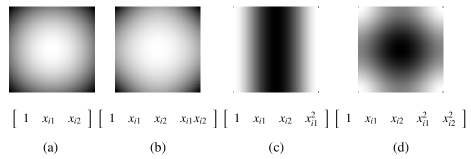
Figure 1: Value of D-optimality criterion as a function of fifth point’s coordinates for different structure of matrix $\bf{Z}$; optimal value is represented by black colour.

To overcome this problem, different approaches have been developed. For instance, the authors in [13] start with a larger Latin Hypercube (LH) design optimised w.r.t. EMM criterion. Then, the final smaller DoE is selected as a combination of points from the previously obtained LH design. In this way, no duplicates are presented, however the optimisation w.r.t. D-optimal criterion is quite perfunctory. Another approach based on a Bayesian modification of an information matrix is proposed in [14]. The idea is to add higher order terms in the response surface approximation and subsequently to add corresponding columns into the matrix ${\bf Z}$. Then, the information matrix $(\bf{Z}^{T}\bf{Z})$ becomes singular, but according to [15], some constant $\tau\in]0,1]$ can be added to diagonal elements of $(\bf{Z}^{T}\bf{Z})$ corresponding to added columns to overcome this problem. The constant $\tau$ is a parameter of the proposed procedure defining the influence of the Bayesian modification, smaller values imply smaller influence. It is not obvious which terms should be added into the matrix ${\bf Z}$, for instance, Figure 1b shows that one term needs not be sufficient, and thus this question should be the subject to additional research. One should keep in mind to add terms equally to all coordinates so as to preserve the isotropy of the resulting DoE, see Figure 1c for an example of anisotropic criterion. In the case of five points in two-dimensional domain, two quadratic terms are sufficient to define DoE without the duplicates, see Figure 1d. The D-optimal designs presented further in this paper are obtained by the described manual Bayesian extension of the information matrix.

2.2 Orthogonality-based criteria

There are two well-know approaches to evaluate the orthogonality of a DoE. The most popular one is based on correlation among the samples’ coordinates, the other one is a condition number.

Condition number (CN) is commonly used in numerical linear algebra to examine the sensitivities of a linear system [16]. Here, we use condition number of ${\bf X}^{T}{\bf X}$, where ${\bf X}$ is a matrix of the design points’ coordinates, so called design matrix

$$\bf{X}=\left[\begin{array}[]{cccc}x_{11}&x_{12}&\cdots&x_{1k}\\ x_{21}&x_{22}&\cdots&x_{2k}\\ \vdots&\vdots&&\vdots\\ x_{n1}&x_{n2}&\cdots&x_{nk}\\ \end{array}\right]\,,$$ (6)

where $n$ is the number of the design points and $k$ is the dimension of the design space and the columns are centered to sum to $0$ and scaled to the range $\left[-1,1\right]$. The condition number is then defined as

$$E^{\mathrm{CN}}=\mbox{cond}(\bf{X}^{T}\bf{X})=\frac{\lambda_{1}}{\lambda_{n}}\,,$$ (7)

where $\lambda_{1}$ and $\lambda_{n}$ are the largest and smallest eigenvalues of ${\bf X}^{T}{\bf X}$, respectively, therefore the $E^{\mathrm{CN}}$ is greater or equal to $1$. Values closer to $1$ correspond to more orthogonal DoE, therefore the condition number should be minimised.

Pearson product-moment correlation coefficient (PMCC) is a standard measure of a linear dependence between two variables. Having two variables $x_{i}$ and $x_{j}$, the PMCC is defined as

$$c_{ij}=\frac{\mathrm{Cov}\left(x_{i},x_{j}\right)}{\sigma_{x_{i}}\sigma_{x_{j}}}=\frac{\sum_{a=1}^{n}(x_{ai}-\overline{x_{i}})(x_{aj}-\overline{x_{j}})}{\sqrt{\sum_{a=1}^{n}(x_{ai}-\overline{x_{i}})^{2}\sum_{a=1}^{n}(x_{aj}-\overline{x_{j}})^{2}}}\,,$$ (8)

where

$$\overline{x_{i}}=\frac{1}{n}\sum_{a=1}^{n}x_{ai}\quad\mbox{ and }\quad\overline{x_{j}}=\frac{1}{n}\sum_{a=1}^{n}x_{aj}\,.$$ (9)

The PMCC takes a value between $-1$ and $1$ and positive values indicate that the value of $x_{i}$ tends to increase together with increasing value of $x_{j}$, while negative values indicate decreasing value of $x_{i}$ with increasing value of $x_{j}$. Zero value stands for no linear relationship between $x_{i}$ and $x_{j}$. In order to obtain orthogonal DoE in a multi-dimensional design space, the PMCC needs to be evaluated for each pair of columns in the design matrix (6). As a result, one obtains a $k\times k$ symmetric correlation matrix

$$\bf{C}=\left[\begin{array}[]{cccc}c_{11}&c_{12}&\cdots&c_{1k}\\ c_{21}&c_{22}&\cdots&c_{2k}\\ \vdots&\vdots&&\vdots\\ c_{k1}&c_{k2}&\cdots&c_{kk}\\ \end{array}\right]\,.$$ (10)

In the case of an orthogonal DoE, the correlation matrix ${\bf C}$ is equal to the identity matrix. To achieve an orthogonal DoE, one can, for instance, minimise the maximum $|c_{ij}|$ as in [16] or the sum of squares of the elements above the main diagonal of ${\bf C}$ as it is done in engineering softwares [17, 18] as well as in presented results, i.e.

$$E^{\mathrm{PMCC}}=\sqrt{\sum_{i=1}^{k}\sum_{j=i+1}^{k}c_{ij}^{2}}\,.$$ (11)

Spearman’s rank correlation coefficient (SRCC) can be used to capture a nonlinear but monotonic relationship between two variables and therefore, it can be efficiently applied for estimation of correlations in sampling-based SA [2]. The idea is to replace the values of $x_{ai}$ and $x_{aj}$ by their corresponding ranks $r(x_{ai})$ and $r(x_{aj})$ and then the SRCC can be computed as

$$\rho_{ij}=1-\frac{6\sum_{a=1}^{n}\left(r(x_{ai})-r(x_{aj})\right)^{2}}{n(n^{2}-1)}\,.$$ (12)

In case of a multi-dimensional design space, the orthogonality of the DoE can be similarly to (11) achieved by minimizing

$$E^{\mathrm{SRCC}}=\sqrt{\sum_{i=1}^{k}\sum_{j=i+1}^{k}\rho_{ij}^{2}}\,.$$ (13)

Kendall tau rank correlation coefficient (KRCC) is an alternative measure of a nonlinear dependence between two variables. In particular, it is based on the number of concordant ($T_{c,ij}$) and discordant ($T_{d,ij}$) pairs of samples according to

$$\tau_{ij}=\frac{T_{c,ij}-T_{d,ij}}{n(n-1)/2}\,,$$ (14)

and again, the orthogonal DoE can be obtained by minimizing

$$E^{\mathrm{KRCC}}=\sqrt{\sum_{i=1}^{k}\sum_{j=i+1}^{k}\tau_{ij}^{2}}\,.$$ (15)

3 Latin Hypercube Sampling

Since the optimisation of DoE defined on real domains becomes computationally exhaustive even at moderate number of dimensions or design points, practical applications are usually restricted to the optimisation of the so called Latin Hypercube (LH) designs [19]. LH sampling provides a possibility to represent prescribed probabilistic distribution of particular variables and hence, it can be efficiently applied in uncertainty analysis [3]. The idea is to divide the range of each variable $x_{j}$ into $n$ disjoint intervals of equal probability and one value $x_{ij}$ is selected from each interval. This selection can be either random or commonly prescribed to the centre of the interval. Then, the $n$ values for each variable are randomly selected without replacement and coupled with $n$ values of other variables resulting in $n$ vectors of variables where each discrete value of each variable is used only once.

The discretisation itself is quite useful for simplification of the optimisation process. Therefore, we focus our attention mainly to the optimisation of DoE in discrete domains assuming that continuous domains are usually also discretised so as to make the optimisation process manageable. Of course, the LH restriction simplifies the optimisation even more, since the search space is significantly reduced. However, it is not obvious whether such restriction excludes the best solutions regarding the objective of SA. Moreover, the LH restriction is not applicable to originally discrete problems, where design variables are defined in different number of discrete values/levels and the so called mixed design is needed. In such a case, the LH restriction has to be somehow modified. When the numbers of levels are equal to multiples of each other, one can easily prescribe the number of points appearing in each level in order to preserve the homogeneity of resulting designs. In other cases, one can prescribe only the minimal number of points appearing in each level [20, 21]. Alternatively, the authors in [22] optimise the mixed design by mixed integer programming method. In our numerical experiments, we generate the LH designs, where the number of points equals the number of levels of one chosen variable and before the evaluation of a criterion, the coordinates of points with different number of levels are simply rounded into the appropriate values. By this way we compare the LH or the mixed LH (mLH) designs with the free (unrestricted) designs in order to investigate the impact of the LH restriction to results of SA.

4 Optimisation of DoE

Efficient generation of optimal DoE is nowadays a subject of an intensive scientific effort. The main reason is that all of the presented criteria are multi-modal functions of optimised variables, hence, gradient-based algorithms cannot be efficiently applied and a robust stochastic algorithm needs to be developed. Let us recall several recent works on this topic: the usage of AE criterion for generating uniform LH designs was recently proposed in [23] and further developed in [21] applying a permutation-based genetic algorithm for optimisation; bounds for maximin LH designs were established in [24] and comparison of suitable generators for the case of EMM criterion are presented in [25]; threshold accepting heuristic is applied in [26] for minimizing the ML₂ discrepancy on LH designs; a review of existing methods for generating space-filling optimal LH designs together with presentation of another heuristic strategy can be found in [27] and simulated annealing was employed for generating LH designs with prescribed correlation matrix in [28]. An important aspect concerns the sequential generation of DoEs which is briefly discussed in Section 7.

Although it is not the aim of the present paper, the efficiency of a particular criterion is, indeed, closely related to the possibility of its optimisation. To sketch the difficulty of generating particular optimal DoE, we present a simple comparison of the presented criteria as functions to be optimised. For the sake of clarity, we present two examples of two-dimensional DoEs with four and five points, where three and four points, respectively, are fixed in the corners of the squared design space and each criterion is evaluated as a function of the last point’s coordinates.

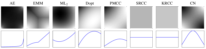
Figure 2: Shape of different criteria for varying position of the 4th point.

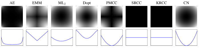
Figure 3: Shape of different criteria for varying position of the 5th point.

Figures 2 and 3 show the shape of the resulting functions in two ways: (i) on the whole domain (the first row) by intensity of grey colour (black colour represents the minimum) corresponding to the value of each criterion at the given position of the last point, and (ii) in more detailed cut of the functional surface according to the diagonal of the domain (the second row). The presented results imply several following conclusions concerning an ease of a corresponding optimisation process.

• SRCC and KRCC as optimisation criteria are by definition discrete functions. When applied to situations with a continuous design space, these functions can have constant value on large subdomains and this phenomenon can make the optimisation process significantly more difficult. Moreover, Figure 3 shows the situation where the optimal value corresponds to a large subdomain of the original space, although the most of randomly chosen solutions from this subdomain cannot be intuitively considered as suitable for SA. Therefore, w.r.t. the presented example, these two criteria can be considered as the most difficult ones to be optimised as well as the criteria poorly defining desired DoE.

• We assume that creation of an excessive number of local extremes can be considered as another negative aspect of optimised criterion. Figure 2 demonstrates that criteria PMCC, CN and Dopt have undesirable local extreme in one of the occupied corner of the design space pointing at the inconvenient character of these criteria. Moreover, the CN criterion evaluates the design with duplicated points in the bottom-right corner to be as good as the design with single point in each corner. That is definitely undesirable, because the design with duplicates is neither orthogonal nor space-filling.

• Other, but less inconvenient, feature of optimised functions is non-smoothness appearing in the case of EMM criterion in both Figures 2 and 3. It was already mentioned that in optimisation of the whole DoE, the all presented criteria become multi-modal and gradient-based methods cannot be efficiently applied. Therefore, it is questionable, how much is the smoothness important when stochastic optimisation methods such as simulated annealing or evolutionary algorithms are employed to solve this problem.

• The last feature arising from the presented examples concerns the ML₂ criterion. From Figure 2 it is clearly visible that the optimal position of the fourth point w.r.t. this criterion is not in the free corner but rather inside the free quadrant of the domain. Such an optimal design is slightly worse in terms of space-filling as well as orthogonality, but it remains the subject of other tests to evaluate the quality of ML₂ criterion w.r.t. usage in SA.

To conclude this section, we would like to point out that the AE criterion seems to have best properties regarding the subsequent optimisation process.

Following sections presents comparisons of DoEs optimised w.r.t. described criteria. Since the designs are not excessively complex, the Simulated Annealing method [29, 30] was applied to optimise each criterion. The procedure slightly differs for the free and for the LH designs. In the first case a single loop of the algorithm involves a sequential selection of a design point and its random movement to any unoccupied position. In the latter case the algorithm randomly chooses two points and then switches one of their randomly chosen coordinates, see [28] for more detailed description of the algorithm implementation for correlation control in small-sample LH designs. The acceptance of a new solution is driven by the Metropolis criterion

$$\exp\left(\frac{f_{\mathrm{old}}-f_{\mathrm{new}}}{T}\right)\geq U\,,$$ (16)

where $f_{\mathrm{old}}$ and $f_{\mathrm{new}}$ stand for values of a criterion for an actual and for a new solution, respectively. $T$ denotes the algorithmic temperature initially set to $T_{\mathrm{max}}=10^{-3}$ and gradually reduced by a multiplicative constant $T_{\mathrm{mlt}}=(\nicefrac{{T_{\mathrm{max}}}}{{10^{-6}}})^{\nicefrac{{1}}{{100}}}$ after each $\nicefrac{{n_{\mathrm{max}}}}{{10}}$ iterations or sooner if the number of accepted movements reaches the value $\nicefrac{{n_{\mathrm{max}}}}{{100}}$. The entire algorithm terminates after $n_{\mathrm{max}}=10^{6}$ objective function evaluations.

Of course, there is no guarantee that the global optimum is achieved, nevertheless, more frequent convergence to local extremes also reflect the shortcoming of a particular criterion. Hence, we decided to present the obtained results without any deeper search for more robust and reliable optimisation method.

5 Comparison of mutual qualities of optimal DoEs

While the presented criteria were originally developed to achieve good space-filling property or orthogonality of the final DoE, it does not mean that the resulting optimal DoE must have bad quality w.r.t. other properties. In order to estimate the mutual quality of individual criteria, we have performed a set of tournament comparisons with small designs having $7$, $10$ and $13$ points in two-dimensional discrete domain. The first variable can only attain $10$ discrete values, while the second variable has possible $7$, $10$ or $13$ values according to the number of design points.

In order to reduce the effect of randomness of the optimisation algorithm, the optimisation process was performed $100$ times for each criterion and the obtained designs were stored and subsequently evaluated by all other criteria. Figures 4 and 5 show statistics over the obtained results in terms of box plots. In Figure 4, each rectangle is devoted to one particular criterion, which is used to evaluate the DoEs obtained by optimizing itself and all other criteria, while in Figure 5, each rectangle contains results of DoEs optimised w.r.t. one criterion and then evaluated by all the other criteria. Repeating the results in Figures 4 and 5 in different arrangement gives us the possibility to more easily formulate distinct conclusions. While the Figure 4 demonstrates the ease of satisfaction of each criterion, the Figure 5 shows the quality of particular optimal DoEs when evaluated by other criteria. Just recall that all the criteria are minimised and smaller values represent better designs.

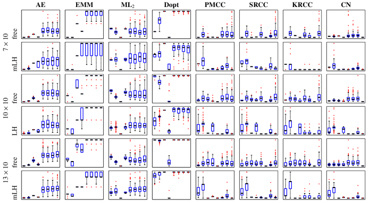
Figure 4: Statistics on results of criteria mutual comparison. Each rectangle contains eight box plots representing the distribution of the values of a criterion associated with the corresponding column. Therefore the scale of each rectangle changes according to the evaluated criterion. Individual box plots correspond to results obtained by optimizing particular criteria. They are ordered in the same way as columns: AE, EMM, ML₂, Dopt, PMCC, SRCC, KRCC and CN. The rows correspond to the size of the design space and the type of a restriction applied on the designs.

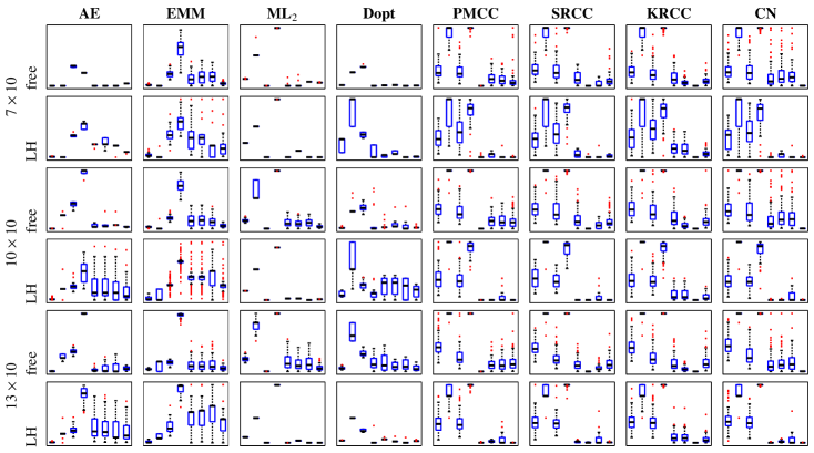
Figure 5: Statistics on results of criteria mutual comparison organised in different way than in Figure 4. Each rectangle contains eight box plots, all corresponding to an optimised criterion associated with the corresponding column. Values in individual box plots are obtained by evaluating particular criteria, ordered in the same way as columns: AE, EMM, ML₂, Dopt, PMCC, SRCC, KRCC and CN. The scale of each box plot is retained the same as in Figure 4. The rows correspond again to the size of the design space and the type of a restriction applied on the designs.

Regarding the results plotted in Figures 4 and 5, the conclusions can be stated as follows:

• The optimal values obtained by optimisation of particular criterion in all of the $100$ runs have very small scatter, which indicates that the global optimum was probably found in most of the cases. It means that Simulated Annealing method is robust enough to solve these optimisation problems in a given time. Thus the results should remain the same even if some other sufficiently robust algorithm is applied.

• The nonorthogonality is easier to be minimised, which is a conclusion consistent with the results derived in [31]. The overall results show that the designs optimised in terms of space-filling property are often nearly orthogonal. On the other hand, the designs optimised w.r.t. the orthogonality display usually bad space-filling and the improvement achieved by LH restriction is negligible. What is more surprising is that the resulting designs are not so well evaluated even by other orthogonality-based criteria.

• The AE and EMM optimal designs exhibit similar properties and good qualities w.r.t. each other. However their quality is not very good in terms of ML₂ and Dopt criteria. The AE optimal designs are slightly more non-orthogonal. The orthogonality of both is deteriorated by applying LH restrictions.

• Dopt criterion is a unique criterion in the sense that all designs optimised w.r.t. all other criteria are very far from being D-optimal. On the other hand, the D-optimal designs are very good regarding the AE criterion and moderate in EMM and ML₂ criteria. These qualities are slightly deteriorated by applying LH restrictions. Regarding the orthogonality of the D-optimal designs, LH restrictions have unclear effect. In general, the D-optimal designs have good or very good level of orthogonality. In the case of 10 design points, LH restriction leads to worsening of the orthogonality, but it leads to an improvement in the case of 13 design points.

• ML₂ optimal designs are slightly worse in terms of AE and EMM criteria then D-optimal designs, but they have good level of orthogonality which is even improved in combination with the LH restriction.

To appreciate the space-filling properties more visually, the resulting optimal DoEs are plotted in Figure 6 together with the corresponding bar charts visualising the distance of each point to its nearest neighbour. The plotted examples are chosen among the other designs for their worst result in the sum of the minimal distances to other points. The aim is to show the worst results one can get by optimizing particular criteria.

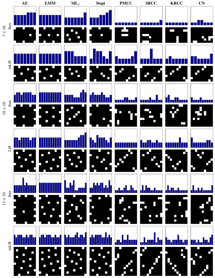
Figure 6: Optimal designs and corresponding bar charts of minimum distances.

6 Projective properties of optimal DoEs

Besides the space-filling and non-orthogonality property, the quality in terms the projective properties is the most crucial in sensitivity analysis. A DoE has good projective properties if each coordinate of each design point is strictly unique [32, 33]. A SA – in the so called screening phase – can often reveal model parameters with a negligible impact on model response. These parameters are then omitted in the following analysis and further application of the created DoE such as in response surface construction. Omitting of some parameters originally involved in constructed DoE implies its projection from $k$-dimensinal space onto $(k-u)$-dimensional space, where $k$ stands for the original number of parameters and $u$ is the number of unimportant parameters to be further neglected. If none of the design points is projected onto another point, the DoE has good projective properties which are alternatively called as non-collapsing property [34]. In an opposite situation, the projection results in smaller DoE with duplicate points and the corresponding simulations are wasted.

An important advantage of Latin Hypercube Sampling (LHS) is that the resulting DoEs have good projective properties given by definition of the LHS itself. Hence, we were interested in a projective properties of free designs optimised w.r.t. the particular criteria. For measuring the quality in terms of projective properties, the authors in [32] use the so called minimum projected distance, which is suitable for DoEs defined in continuous domains. For case of discrete domains, we use simply the number of redundant points. To that purpose, we have projected all the optimal designs presented in the previous section onto the dimension discretised into $10$ values. The obtained results are plotted in Figure 7 in terms of histograms representing the number of DoEs with the given number of redundant points.

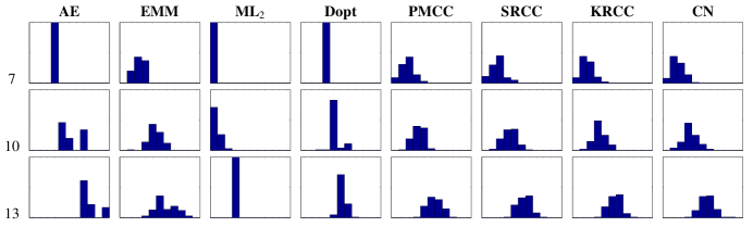
Figure 7: Histograms of redundant points in projected DoEs. The horizontal axis corresponds to the number of redundant points from $0$ to $10$, while the vertical axis represents the number of DoEs with the given number of redundant points from $0$ to $100$. Rows correspond to the number of levels of the variable left out. Columns correspond again to particular criteria.

For an easier interpretation of the results, the average number of redundant points are listed in Table 1.

	AE	EMM	ML2	Dopt	PMCC	SRCC	KRCC	CN
$7$	3,00	2,17	0,00	3,00	1,71	1,67	1,52	1,56
$10$	5,22	4,37	0,32	4,23	3,22	3,33	3,24	3,29
$13$	7,73	5,81	3,00	5,20	5,42	5,32	5,35	5,57
celkem	5,32	4,12	1,11	4,14	3,45	3,44	3,37	3,47

Table 1: Average number of redundant simulations.

The results show the superiority of ML₂ designs containing minimal number of redundant points in projected designs. Worst results were obtained for other space-filling designs.

7 Sequential generation of DoEs

Before generation of a desired DoE, one has to make a decision about the number of design points. In case of a discrete problem, the decision usually follows the number of variable levels, while in continuous problems, the only clue is usually the available time for running the simulations. The authors in [33] consider so called granularity as an important property of a DoE generation strategy. A fine-grained sequential strategy adds just a few points in each iteration, while the coarse-grained adds new points in large batches. Methods allowing only one iteration produce so called one-shot DoEs. The principal advantage of fine-grained sequential strategy is the possibility to avoid the generation of too many samples which are not necessary (i.e. oversampling) or too few samples which are not sufficient to achieve the desired accuracy (i.e. undersampling). On the other hand, the advantage of one-shot DoEs is generally their better quality in terms of space-filling or non-orthogonality and of course in terms of any chosen criterion. However, the optimisation of a large design can be more complex and the obtained locally optimal design may display worse properties then coarse-grained sequentially produced design.

The authors in [33] present a review of a different procedures for one by one generated sequential designs and compare their qualities with one-shot DoEs in terms of space-filling and non-orthogonality property. The presented methods are searching new points position in continuous domain or in a sequentially refined grid in order to provide a Latin Hypercube-like designs. The latter idea is elaborated and tested in more detail e.g. in [35]. All these methods are stochastic and in each iteration, some sort of optimisation process is applied in order to increase the space-filling or non-orthogonality of the DoE.

Another type of methods are purely deterministic, such as factorial designs [36] or methods used for numerical integration such as sparse grids, see e.g. [37, 38]. The advantage of these pre-optimised sequential designs is very fast generation free of any optimisation at every iteration. The cost is of course generally worse space-filling or non-orthogonality.

Last group of methods we should mention consists of strategies employed in response surface modelling, where the new sample points are placed where the response surface is supposed to have large error, see e.g. [39] or [40]. However, in sensitivity analysis we cannot use any such additional information. Moreover, in sensitivity analysis it is also much harder to estimate the accuracy of the sensitivity predictions and decide whether the DoE is large enough. One way is to compute the bootstrap confidence intervals, see e.g. [41].

In this paper, we do not presume to discuss this broad topic in more details and we focus only on sequential designs in discrete domains, where the grid is fixed. Therefore, we employed two strategies, where the number of new points is equal to the number of levels in discrete domain and remains the same in all iterations. At each iteration, the positions of new points are optimised w.r.t. the chosen criterion, which is always evaluated for the whole design. The designs presented in Section 4 are used as a starting DoEs and the sequential strategy is applied to each of $100$ DoEs in order to limit again the randomness of the optimisation algorithm.

The first strategy is based on free selection of new points according to the optimized criterion and the free DoEs were employed as initial ones, see Figures 8. The plotted examples are chosen among the other designs for their worst result in the sum of the minimal distances to other points. The aim is to show the worst results one can obtain by optimizing particular criteria.

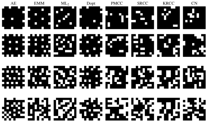
Figure 8: Sequential free designs.

The second strategy starts from the LH designs and preserves the LH constrains also for the added points and thus, the equal number of points are located in each column or row. The resulting DoEs obtained by this method are presented in Fig. 9.

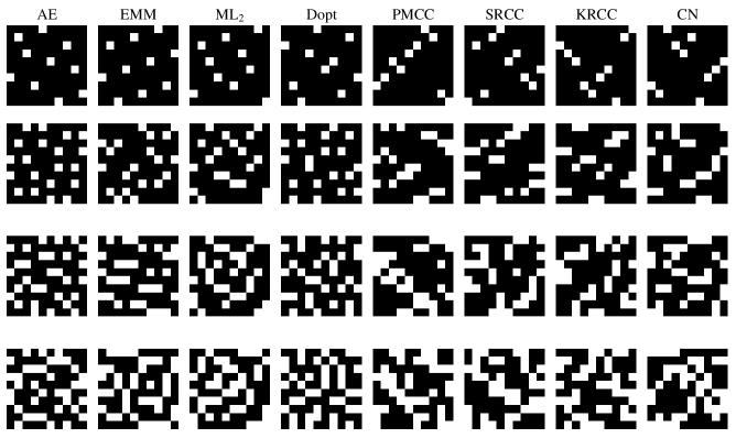
Figure 9: Sequential LH designs.

The quality of the presented designs is examined directly within the sensitivity analysis presented in the following section.

8 Sensitivity analysis on a set of analytical functions

Although the SRCC criterion achieved bad results for generating optimal DoE, it has been shown that it can significantly improve the results in estimating the importance of model parameters in sensitivity analysis for the case of nonlinear monotonic models [2].

Having the numerical model given as

$$z=f(x_{1},x_{2},\dots,x_{k})$$ (17)

relating the model response $z$ and the model parameters $x_{i}$, the impact of the parameter $x_{i}$ to the model response $z$ can be estimated by evaluating their Spearman’s rank correlation $\rho_{x_{i},z}$ according to

$$\rho_{x_{i},z}=1-\frac{6\sum_{a=1}^{n}\left(r(x_{ai})-r(z_{a})\right)^{2}}{n(n^{2}-1)}\,,$$ (18)

where $x_{ai}$ are values of particular model parameter corresponding to points in DoE and $z_{a}$ are values of model responses corresponding to these points.

In engineering practice, the majority of the numerical models fulfil the condition of a monotonic relationship between the model parameters and the model response. Therefore, to support the study of optimal DoE quality in sampling-based SA, we performed the same comparison for a list of nonlinear but monotonic models. In particular, we consider the two-parametric models with discrete parameters, one with $10$ feasible discrete values and the second attaining $7$, $10$ or $13$ feasible discrete values according to the employed DoE. The shapes of the chosen models plotted for the case of square $10\times 10$ domain are shown in Figure 10 together with corresponding parameter-response correlations obtained for the Full design consisting of all feasible design points (here $100$ points).

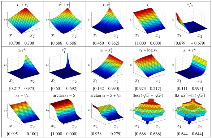
Figure 10: Shapes of 15 functions for sensitivity analysis with the corresponding values of parameter-response correlations.

Then, the parameter-response correlations were estimated using the all optimal designs involved in the mutual comparison in the previous section and the differences among correlations $\tilde{\rho}$ obtained by the optimal designs and correlations $\rho$ obtained by the full designs are stored. The error measure $\epsilon$ in the parameter-response correlations evaluated for a given function is considered as an average difference between each parameter and model response correlation obtained by an optimal and a full design, i.e.

$$\epsilon=\frac{1}{k}\sum_{i=1}^{k}|\tilde{\rho}_{x_{i},z}-\rho_{x_{i},z}|\,.$$ (19)

The statistics over the obtained values of errors $\epsilon$ is presented in Figures 11 and 12 again using the box plots.

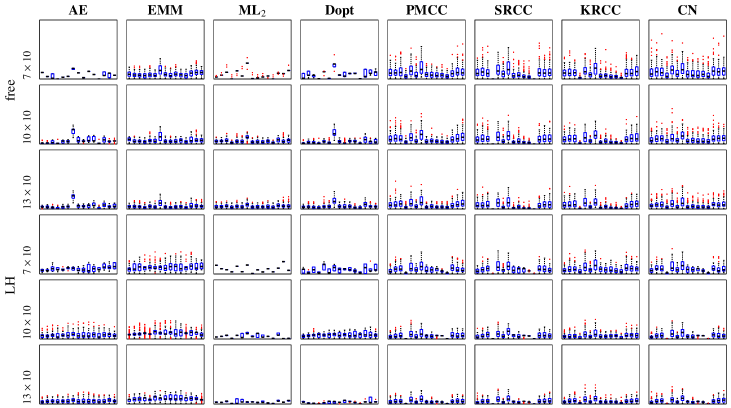
Figure 11: Statistics on results of criteria in estimating parameter-response correlations for analytical models. Each rectangle contains $15$ box plots representing the distribution of errors in correlation prediction for particular models depicted in Figure 10. The scale is $0$ at the bottom and $1$ at the top per rectangle. Furthermore, each rectangle refers to the optimal designs according to one criterion associated with the corresponding column and to the chosen size of the design space and the type of restriction applied associated with the corresponding row.

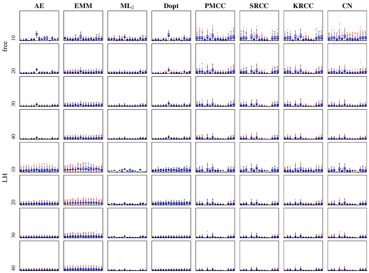
Figure 12: Statistics on sequential DoEs in estimating parameter-response correlations for analytical models. Each rectangle contains $15$ box plots representing the distribution of errors in correlation prediction for particular models depicted in Figure 10. The scale is $0$ at the bottom and $1$ at the top per rectangle. Furthermore, each rectangle refers to the optimal designs according to one criterion associated with the corresponding column and to the chosen number of the design points and the type of restriction applied associated with the corresponding row.

For an easier evaluation of particular criteria, the mean and maximal errors over all models multiplied by $100$ are listed in Tables 2 and 3.

		AE		EMM		ML2		Dopt		PMCC		SRCC		KRCC		CN
		mean	max	mean	max	mean	max	mean	max	mean	max	mean	max	mean	max	mean	max
free	$7\times 10$	6.7	18.0	8.5	34.5	8.4	36.3	7.8	41.2	10.5	59.3	9.7	60.8	9.4	51.8	12.2	76.6
	$10\times 10$	5.9	32.0	6.2	29.4	5.1	20.5	4.5	33.6	8.4	51.4	7.3	48.5	7.5	46.5	8.6	59.9
	$13\times 10$	5.3	30.8	4.7	24.9	4.6	20.8	4.8	29.7	6.8	47.1	5.6	37.0	6.1	39.9	6.9	39.6
	overall	6.0	32.0	6.5	34.5	6.0	36.3	5.7	41.2	8.6	59.3	7.5	60.8	7.7	51.8	9.2	76.6
LH	$7\times 10$	9.0	20.6	11.9	37.3	8.5	20.8	7.0	21.9	7.6	37.3	7.4	39.1	8.8	40.5	7.9	42.9
	$10\times 10$	6.7	28.9	9.8	31.1	4.5	11.2	6.8	20.3	5.5	31.4	5.8	28.4	5.6	33.0	5.3	30.7
	$13\times 10$	5.2	20.0	8.7	22.5	3.3	8.9	2.8	11.6	4.4	22.7	4.3	24.9	4.9	32.2	4.6	29.1
	overall	7.0	28.9	10.1	37.3	5.4	20.8	5.5	21.9	5.8	37.3	5.8	39.1	6.4	40.5	5.9	42.9

Table 2: Mean and maximal errors of one-shot DoEs in correlation predictions for analytical models.

		AE		EMM		ML2		Dopt		PMCC		SRCC		KRCC		CN
	points	mean	max	mean	max	mean	max	mean	max	mean	max	mean	max	mean	max	mean	max
free	10	5.9	32.0	6.2	29.4	5.1	20.5	4.5	33.6	8.4	51.4	7.3	48.5	7.5	46.5	8.6	59.9
	20	3.3	16.5	4.6	19.7	3.1	14.3	2.9	20.7	5.1	34.2	4.4	32.4	4.4	29.9	4.4	37.4
	30	2.1	12.0	4.3	17.1	2.2	10.6	3.0	17.4	3.6	25.2	3.3	22.7	3.2	26.1	2.9	22.0
	40	1.5	10.0	4.1	16.0	1.7	8.5	2.5	13.0	2.6	19.0	2.4	23.4	2.5	19.6	2.2	17.0
	overall	3.2	17.6	4.8	20.6	3.0	13.5	3.2	21.2	4.9	32.5	4.4	31.8	4.4	30.5	4.5	34.1
LH	10	6.7	28.9	9.8	31.1	4.5	11.2	6.8	20.3	5.5	31.4	5.8	28.4	5.6	33.0	5.3	30.7
	20	4.8	15.4	7.1	25.3	2.8	10.2	6.0	19.3	3.1	20.8	3.1	18.5	3.0	18.6	3.0	25.2
	30	2.6	11.3	5.3	22.9	2.3	8.7	2.5	9.6	2.1	21.8	2.2	18.2	2.3	17.5	2.2	20.5
	40	2.5	9.0	4.9	19.2	1.6	5.9	2.3	8.8	1.6	11.3	1.6	12.6	1.8	15.5	1.7	15.1
	overall	4.2	16.2	6.8	24.6	2.8	9.0	4.4	14.5	3.1	21.3	3.2	19.4	3.2	21.2	3.1	22.9

Table 3: Mean and maximal errors of sequential DoEs in correlation predictions for analytical models.

The results on the sampling-based SA for analytical models can be summarised as follows:

• The overall best results were achieved by the ML₂ optimal LH designs in terms of the average achieved errors as well as in their small variance. The results of the ML₂ optimal free designs were slightly worse and comparable to D-optimal designs. Free variant of both designs suffer from larger variance.

• The AE and EMM criteria provided in average much better free designs comparing the their LH variant. However the variance is high for both of them. The quality of AE optimal free design can be classified as very good and comparable to results obtained by ML₂ and Dopt criteria. On the other hand EMM criterion provided relatively bad designs, which were only very slowly improved by their sequential extension.

• On the contrary, the orthogonality-based criteria achieved much better results for LH designs comparing to their free variant. All of these criteria provided comparable LH designs and can be evaluated as very good. However, their predictions suffer from very large variance.

9 Sensitivity analysis on truss structures

The sensitivity analysis study presented in the previous section is aimed on two-dimensional analytical problems. Therefore, this section is devoted to illustrative engineering problems with higher dimensions. We have chosen two models of truss structures commonly used as benchmarks for sizing optimisation.

The first one represents a ten-bar truss structure [42] shown in Figure 13. The design variables are the cross-sectional areas of the bars. This benchmark is defined with two types of variables: continuous and discrete one. Here we focus on a discrete formulation with discrete values of cross-sectional areas together with values of material properties and loading taken from [43]. All ten cross-sectional areas have the same $42$ feasible discrete values (in²): 1.62, 1.80, 1.99, 2.13, 2.38, 2.62, 2.63, 2.88, 2.83, 3.09, 3.13, 3.38, 3.47, 3.55, 3.63, 3.84, 3.87, 3.88, 4.18, 4.22, 4.49, 4.59, 4.80, 4.97, 5.12, 5.74, 7.22, 7.97, 11.50, 13.50, 13.90, 14.20, 15.50, 16.00, 16.90, 18.80, 19.90, 22.00, 22.90, 26.50, 30.00, 33.50.

Material:	Aluminum
Specific weight:	0.1 lb/in3
Young’s modulus:	$10^{7}$ psi
Loading P:	100 kips

Figure 13: Scheme of a ten-bar truss structure together with material parameters and values of applied loading.

The second model concerns a 25-bar truss structure with a geometry, material properties and loading given in Figure 14. Thanks to the symmetry of the structure, the bars can be organised into eight groups. The bars in one group have the same cross-sectional areas and hence, there are only eight design variables. These variables are again discrete with $30$ feasible values (in²): 0.1, 0.2, 0.3, 0.4, 0.5, 0.6, 0.7, 0.8, 0.9, 1.0, 1.1, 1.2, 1.3, 1.4, 1.5, 1.6, 1.7, 1.8, 1.9, 2.0, 2.1, 2.2, 2.3, 2.4, 2.5, 2.6, 2.8, 3.0, 3.2, 3.4, see [44].

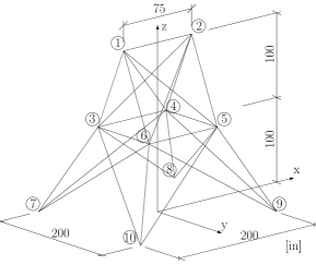
Material:	Aluminum
Specific weight:	0,1 lb/in3
Young’s modulus:	$10^{7}$ psi

Nodal loads
Node	Fx	Fy	Fz
1	1.0	-10.0	-10.0
2	0.0	-10.0	-10.0
3	0.5	0.0	0.0
6	0.6	0.0	0.0

Figure 14: Scheme of a 25-bar truss structure together with material parameters and values of applied loading.

The response of these models consists of three components: total weight of the structure $w$, maximal deflection $d$ and maximal stress $s$. Because of higher dimensions of these problems, we have generated the optimal DoEs only with LH restriction, since they can be optimised more easily. This restriction automatically specifies the number of corresponding design points, which has to be equal to the number of feasible values ($42$ for the ten-bar truss and $30$ for the 25-bar truss) or their multiples in case of sequential designs.

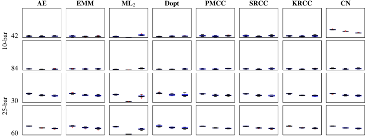
Figure 15: Statistics on results in estimation of parameter-response correlations for structural models. Each rectangle contains three box plots representing the distribution of the errors in correlation prediction for particular model responses: the total weight $w$, the maximal deflection $d$ and the maximal stress $s$. The scale is $0$ at the bottom and $1$ at the top per rectangle. Each rectangle refers to optimal designs according to one criterion associated with the corresponding column and to the chosen structure and number of design points associated with the corresponding row.

A simulated annealing method with the same parameters as described in Section 5 but with a maximum of $10^{7}$ iterations was employed to generate $20$ optimal DoEs using each criterion under the study. The parameter-response correlations were then estimated using the obtained optimal DoEs and compared with the correlations computed using the Large DoEs consisting of $2\cdot 10^{7}$ samples generated by the Monte Carlo method. The statistics on the errors $\epsilon$ in estimation of parameter-response correlations is demonstrated again in terms of box plots independently for each criterion and each model response component, see Figure 15.

For a clearer summary of the obtained results, the mean and maximal errors in correlation predictions multiplied again by $100$ are listed in Table 4.

Model			AE		EMM		ML2		Dopt		PMCC		SRCC		KRCC		CN
			mean	max	mean	max	mean	max	mean	max	mean	max	mean	max	mean	max	mean	max
10-bar	42	$w$	5.1	7.5	4.9	7.5	4.1	5.5	4.3	5.4	6.2	10.3	5.9	9.2	5.8	7.5	27.0	29.7
		$d$	4.5	6.7	4.4	5.6	0.7	1.1	4.6	6.5	4.5	7.3	4.3	6.2	4.7	7.1	21.7	23.0
		$s$	5.1	7.3	4.7	7.7	8.9	13.9	5.1	8.0	6.5	9.2	6.8	11.0	6.6	10.7	15.7	17.7
		overall	4.9	7.5	4.7	7.7	4.6	13.9	4.7	8.0	5.7	10.3	5.7	11.0	5.7	10.7	21.5	29.7
	84	$w$	3.9	5.1	4.1	6.1	2.3	3.6	3.0	4.2	3.7	6.3	3.9	6.1	4.1	5.8	5.4	7.7
		$d$	2.7	3.6	3.6	6.7	0.4	0.7	2.9	4.0	3.1	5.0	2.7	4.6	2.9	4.4	3.4	5.5
		$s$	3.3	5.7	3.9	6.0	5.4	7.7	3.7	5.8	5.0	6.7	4.3	7.7	4.4	8.0	4.8	8.0
		overall	3.3	5.7	3.9	6.7	2.7	7.7	3.2	5.8	3.9	6.7	3.6	7.7	3.8	8.0	4.5	8.0
25-bar	30	$w$	30.0	32.3	30.4	33.5	26.8	28.9	31.6	38.3	29.5	30.8	29.6	30.7	29.9	31.4	30.0	31.2
		$d$	24.6	27.2	25.1	27.5	23.6	28.3	26.8	35.7	24.4	28.1	24.1	27.1	24.3	25.8	24.5	27.2
		$s$	22.6	25.9	23.2	27.6	21.2	27.4	25.2	33.4	23.8	27.2	23.0	26.0	22.7	25.8	23.4	26.3
		overall	25.7	32.3	26.2	33.5	23.9	28.9	27.9	38.3	25.9	30.8	25.6	30.7	25.6	31.4	26.0	31.2
	60	$w$	30.0	30.9	30.0	31.9	27.8	29.5	30.2	34.1	29.4	30.4	29.4	30.4	29.9	31.4	29.9	30.9
		$d$	23.9	25.1	24.7	27.7	22.5	25.5	24.9	27.3	23.8	25.3	23.6	25.6	24.2	26.5	23.8	25.1
		$s$	21.6	23.7	22.3	25.8	19.3	22.6	22.6	26.4	22.1	23.9	21.9	23.9	22.5	25.1	22.2	23.8
		overall	25.2	30.9	25.7	31.9	23.2	29.5	25.9	34.1	25.1	30.4	25.0	30.4	25.5	31.4	25.3	30.9

Table 4: Mean and maximal errors in correlation predictions for structural models.

To conclude the obtained results on the sampling-based SA for structural models we can formulate following points:

• Apart from the CN optimal designs, all the other designs achieved very good results in predicting sensitivities for the ten-bar truss structure. The CN designs achieved surprisingly bad results in predicting sensitivities to all three response components. Nevertheless, these results were significantly improved by extension of the design.

• All space-filling criteria achieved better results for the ten-bar truss structure than all orthogonality based criteria. The smallest mean error in prediction was obtained by the ML₂ designs, however it is accompanied by relatively big differences among errors corresponding to particular response components. The AE, EMM and Dopt designs provided more balanced results.

• We are not able to find differences among the studied criteria based on the results for the $25$-bar structure. Obviously, the model is too complex to estimate the parameter-response sensitivities using the design with only $30$ or $60$ points in the eight-dimensional design space and hence, all the criteria led to comparably bad predictions.

10 Conclusions

This paper reviews eight criteria used for optimizing a design of experiments and presents their comparison in terms of ease of their optimisation, their mutual qualities and their suitability for usage in sampling-based SA on $15$ analytical and two structural models. The overall results can be summarised in several following conclusions:

• CN criterion was poorly evaluated in terms of all presented aspects. It may make the optimisation process more complicated by its tendency to the higher number of local extremes. The resulting designs have very poor space-filling properties and the subsequent sensitivity predictions for analytical as well as for structural models contain large errors.

• The correlation-based criteria (PMCC, SRCC and KRCC) may also pose some difficulties during the optimisation process: SRCC and KRCC due to their discrete nature and PMCC due to its stronger tendency to the multi-modality. All these criteria provide the designs with very bad space-filling property and even LH restriction does not improve it significantly. While the free designs achieved also very bad results in SA, the predictions of LH designs can be evaluated as very good, but they suffer from higher variances.

• AE and EMM criteria do not exhibit any explicit difficulties regarding the optimisation process. The advantage of these criteria is that their interpretation is very simple and computation very fast. They provide designs with similar properties: good space-filling and a moderate level of orthogonality. The free designs achieved good results in sensitivity predictions but also with a high variance among the results. The results of EMM criterion are in overall worse then those of AE criterion. Their qualities are generally deteriorated by applying the LH restriction.

• Finally, the best results in sensitivity predictions were obtained using the LH designs optimised w.r.t. the ML₂ criterion. The D-optimal designs were slightly worse and comparable to AE free designs or LH designs optimised w.r.t. the correlation-based criteria. ML₂ and Dopt criteria provide designs with moderate space-filling properties, but they have a good level of orthogonality. The LH restriction slightly improves the results of both. The ML₂ designs achieved less varying results in the SA for analytical functions, while the D-optimal designs provided more balanced results in the SA for the ten-bar truss structure. The ML₂ designs also significantly overcame all the other designs in terms of the projective properties. An important shortcoming of the D-optimal criterion concerns its formulation and optimisation. Besides the fact that the criterion results in an excessive number of local extremes, the principal drawback lies in the necessity of its Bayesian modification for elimination of duplicates or closely neighbouring points. Therefore, the ML₂ criterion, which is not so common in DoE optimisation, can be considered as a winner in the presented competitive comparisons.

References

- [1] A. Kučerová, Identification of nonlinear mechanical model parameters based on softcomputing methods, Ph.D. thesis, Ecole Normale Supérieure de Cachan, Laboratoire de Mécanique et Technologie (2007).
- [2] J. C. Helton, J. D. Johnson, C. J. Sallaberry, C. B. Storlie, Survey of sampling-based methods for uncertainty and sensitivity analysis, Reliability Engineering & System Safety 91 (10-11) (2006) 1175–1209.
- [3] J. C. Helton, J. D. Johnson, W. L. Oberkampf, C. J. Sallaberry, Sensitivity analysis in conjunction of with evidence theory representations epistemic uncertainty, Reliability Engineering & System Safety 91 (10-11) (2006) 1414–1434.
- [4] A. Saltelli, K. Chan, E. M. Scott, Sensitivity analysis, NY:Wiley, New York, 2000.
- [5] T. Goel, R. T. Haftka, W. Shyy, L. T. Watson, Pitfalls of using a single criterion for selecting experimental designs, International Journal for Numerical Methods in Engineering 75 (2) (2008) 127–155.
- [6] P. Audze, V. Eglais, New approach for planning out of experiments, Problems of Dynamics and Strengths 35 (1977) 104–107, Zinatne Publishing House.
- [7] M. Johnson, L. Moore, D. Ylvisaker, Minimax and maximin distance designs, Journal of Statistical Planning and Inference 26 (2) (1990) 131–148.
- [8] M. D. Morris, T. J. Mitchell, Exploratory designs for computer experiments, Journal of Statistical Planning and Inference 43 (3) (1995) 381–402.
- [9] K. T. Fang, Y. Wang, Number-theoretic Methods in Statistics, Chapman & Hall, London, 1994.
- [10] S. Heinrich, Efficient algorithms for computing the -discrepancy, Mathematics of Computation 65 (216) (1996) 1621–1633.
- [11] K. Smith, On the standard deviations and interpolated values of an observed polynomial function and its constants and the guidance they give towards a proper choice of the distribution of observations, Biometrika 1/2 (1918) 1–85.
- [12] P. F. de Aguiar, B. Bourguignon, M. S. Khots, D. L. Massart, R. Phan-Than-Luu, D-optimal designs, Chemometr Intell Lab 30 (2) (1995) 199–210.
- [13] T. Goel, R. T. Haftka, W. Shyy, Comparing error estimation measures for polynomial and kriging approximation of noise-free functions, Structural and Multidisciplinary Optimization 38 (5) (2009) 429–442.
- [14] M. Hofwing, N. Strömberg, D-optimality of non-regular design spaces by using a Bayesian modification and a hybrid method, Structural and Multidisciplinary Optimization 42 (1) (2010) 73–88.
- [15] W. DuMouchel, B. Jones, A simple Bayesian modification of D-optimal designs to reduce dependence on an assumed model, Technometrics 36 (1) (1994) 37–47.
- [16] T. M. Cioppa, T. W. Lucas, Efficient Nearly Orthogonal and Space-Filling Latin Hypercubes, Technometrics 49 (1) (2007) 45–55.
- [17] J. Novák, Generator of optimal LHS designs SPERM v. 2.0., Centre for Integrated Design of Advanced Structures (CIDEAS), Czech Technical University in Prague (2011).
- [18] D. Novák, M. Vořechovský, M. Rusina, FREET v. 1.5 - program documentation, Brno/Červenka consulting, Prague, user’s and theory guides Edition (2011).
- [19] R. L. Iman, W. J. Conover, Small sample sensitivity analysis techniques for computer models, with an application to risk assessment, Communications in Statistics - Theory and Methods A9 (17) (1980) 1749–1842.
- [20] F. M. Alam, K. R. McNaught, T. J. Ringrose, A comparison of experimental designs in the development of a neural network simulation metamodel, Simulation Modelling Practice and Theory 12 (7-8) (2004) 559–578.
- [21] V. V. Toropov, S. J. Bates, O. M. Querin, Generation of Extended Uniform Latin Hypercube Designs of Experiments, in: B. Topping (Ed.), Proceedings of the Ninth International Conference on the Application of Artificial Intelligence to Civil, Structural and Environmental Engineering, Civil-Comp Press, Stirlingshire, Scotland, 2007.
- [22] H. Vieira, S. Sanchez, K. H. Kienitz, M. C. N. Belderrain, Generating and improving orthogonal designs by using mixed integer programming, European Journal of Operational Research 215 (3) (2011) 629–638.
- [23] S. J. Bates, J. Sienz, D. S. Langley, Formulation of the Audze-Eglais Uniform Latin Hypercube design of experiments, Advances in Engineering Software 34 (8) (2003) 493–506.
- [24] E. R. van Dam, G. Rennen, B. Husslage, Bounds for Maximin Latin Hypercube Designs, Operations Research 57 (3) (2009) 595–608.
- [25] E. Myšáková, M. Lepš, Comparison of space-filling design strategies, in: Proc. of Engineering Mechanics 2011.
- [26] K. T. Fang, C.-X. Ma, P. Winker, Centered -discrepancy of Random Sampling and Latin Hypercube Design, and Construction of Uniform Designs, Mathematics of Computation 71 (237) (2002) 275–296.
- [27] F. A. C. Viana, G. Venter, V. Balabanov, An algorithm for fast optimal Latin hypercube design of experiments, International Journal for Numerical Methods in Engineering 82 (2) (2010) 135–156.
- [28] M. Vořechovský, D. Novák, Correlation control in small-sample Monte Carlo type simulations I: A simulated annealing approach, Probabilistic Engineering Mechanics 24 (3) (2009) 452–462.
- [29] S. Kirkpatrick, C. Gelatt, Jr., M. P. Vecchi, Optimization by simulated annealing, Science 220 (1983) 671–680.
- [30] J. Černý, Thermodynamical approach to the traveling salesmanproblem: An efficient simulation algorithm, Journal of Optimization Theory and Applications 45 (1985) 41–51.
- [31] M. Vořechovský, Correlation control in small sample Monte Carlo type simulations II: Analysis of estimation formulas, random correlation and perfect uncorrelatedness, Probabilistic Engineering Mechanics 29 (2012) 105–120.
- [32] D. Bursztyn, D. M. Steinberg, Comparison of designs for computer experiments, Journal of Statistical Planning and Inference 136 (3) (2006) 1103–1119.
- [33] K. Crombecq, E. Laermans, T. Dhaene, Efficient space-filling and non-collapsing sequential design strategies for simulation-based modeling, European Journal of Operational Research 214 (3) (2011) 683–696.
- [34] E. R. van Dam, B. Husslage, D. den Hertog, H. Melissen, Maximin Latin Hypercube Designs in Two Dimensions, Operations Research 55 (1) (2007) 158–169.
- [35] M. Vořechovský, Hierarchical subset latin hypercube sampling for correlated random vectors, in: B. Topping, Y. Tsompanakis (Eds.), Proceedings of the First International Conference on Soft Computing Technology in Civil, Structural and Environmental Engineering, Civil-Comp Press, Stirlingshire, Scotland, 2009.
- [36] D. C. Montgomery, Design and Analysis of Experiments, John Wiley & Sons, New York, 1994.
- [37] S. A. Smolyak, Quadrature and interpolation formulas for tensor products of certain classes of functions, Doklady Akademii Nauk SSSR 4 (1963) 240–243.
- [38] A. Keese, H. G. Matthies, Numerical methods and Smolyak quadrature for nonlinear stochastic partial differential equations, Informatikbericht 2003-5, Institute of Scientific Computing, Department of Mathematics and Computer Science, Technische Universität Braunschweig, Brunswick (2003).
- [39] D. R. Jones, M. Schonlau, W. J. Welch, Efficient global optimization of expensive black box functions, Journal of Global Optimization 13 (1998) 455–492.
- [40] J. S. Lehman, T. J. Santner, W. I. Notz, Designing computer experiments to determine robust control variables, Statistica Sinica 14 (2004) 571–590.
- [41] B. Efron, R. J. Tibshirani, An Introduction to the Bootstrap, Chapman & Hall, New York, 1993.
- [42] V. B. Venkaya, Design of optimum structures, Computers and Structures 1 (1971) 265–309.
- [43] A. C. C. Lemonge, H. J. C. Barbosa, An adaptive penalty scheme for genetic algorithms in structural optimization, International Journal for Numerical Methods in Engineering 59 (2003) 703–736.
- [44] S.-J. Wu, P.-T. Chow, Steady-state genetic algorithms for discrete optimization of trusses, Computers and Structures 56 (6) (1995) 979–991.