On the radial expansion of tubular structures in a quark gluon plasma

Abstract

We study the radial expansion of cylindrical tubes in a hot QGP. These tubes are treated as perturbations in the energy density of the system which is formed in heavy ion collisions at RHIC and LHC. We start from the equations of relativistic hydrodynamics in two spatial dimensions and cylindrical symmetry and perform an expansion of these equations in a small parameter, conserving the nonlinearity of the hydrodynamical formalism. We consider both ideal and viscous fluids and the latter are studied with a relativistic Navier-Stokes equation. We use the equation of state of the MIT bag model. In the case of ideal fluids we obtain a breaking wave equation for the energy density fluctuation, which is then solved numerically. We also show that, under certain assumptions, perturbations in a relativistic viscous fluid are governed by the Burgers equation. We estimate the typical expansion time of the tubes.

I Introduction

The study of the initial stage of relativistic heavy ion collisions has experienced a fast progress in recent years. One of the most interesting findings in this study, supported both by theoretical works and by the analysis of experimental data, is that in the early times of these collisions color flux tubes are formed. Although color flux tubes are familiar objects in hadron physics it is not obvious that they should be formed in high energy heavy ion collisions, where projectile and target can be regarded as bunches of partons without any strong clustering neither in configuration nor in color space. Flux tubes, sometimes called strings, appear in lattice QCD calculations as field configurations between static heavy charges. They appear also in phenomenological models of high energy soft hadronic scattering. In the Lund model, for example, when two high energy protons collide with low momentum transfer, they cross each other and, due to gluon exchange, a color rearrangement takes place with the subsequent formation of strings, which stretch and decay, producing particles.

At high energies, colliding nuclei are dense systems in which the standard linear evolution equations (such as the DGLAP equations) must be replaced by others, which include nonlinear effects in the evolution. The theoretical description of these dense systems evolved into the theory of the Color Glass Condensate (CGC). In this formalism the dense gluonic matter is treated in a semi-classical approximation. In this approach, it has been shown in cgc1 ; cgc2 ; cgc3 ; cgc4 that there are solutions of the classical Yang-Mills equations in which the lines of the chromo-electric and chromo-magnetic fields are all parallel to the collision axis and these fields form color flux tubes in the longitudinal (z) direction.

The interpretation of RHIC and LHC data also suggests that the system reaches thermal equilibrium, forming a thermalized quark-gluon plasma (QGP), very soon after the collision. At first sight this would imply that the flux tubes disappear and the quark-gluon matter becomes reasonably homogeneous when the hydrodynamical expansion starts. However detailed hydrodynamical studies hamatube ; andrade strongly suggest that some experimental features observed at RHIC and LHC can be understood if we assume that these tubes survive the thermalization stage and form “tubular” structures that persist for some time during the hydrodynamical expansion. More specifically, the data show the existence of structures in the two-particle correlations plotted as function of the pseudorapidity difference $\Delta\eta$ and the angular spacing $\Delta\phi$. In hamatube ; andrade it has been argued that these structures may have a common hydrodynamic origin: the combined effect of longitudinal high energy density tubes (leftover from initial particle collisions) and transverse expansion.

The tubular structures described above, which are nearly uniform in the longitudinal direction, may be considered as cylindrical perturbations in the energy density upon a continuous background as depicted in Fig. 1. The propagation of perturbations on the top of a QGP background has been investigated in several works shuryak1 ; shuryak2 ; fn5 ; fn7 . In most of these works shuryak1 ; shuryak2 a linearized version of hydrodynamics is employed. We have tried to keep the nonlinear terms in the equations which describe the evolution of the perturbations fn5 ; fn7 . This extends the validity of our formalism to perturbations which are not so small.

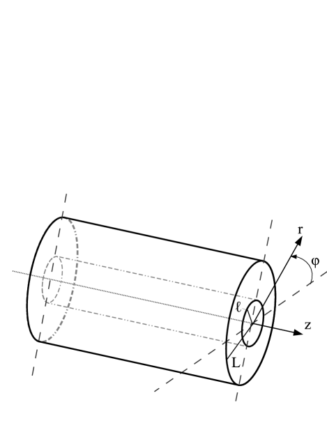
Figure 1: Tubular perturbations on a QGP background. The inner cylinder of radius $l$ represents a tube of energy density higher than the background, shown as a cylindrical fireball of radius $L$. The perturbation expands radially.

In this work we try to answer the question: how fast do the tubes expand in the QGP ? In order to obtain the answer we write the hydrodynamical equations for the propagation of cylindrical perturbations along the radial direction (see Fig. 1), solve them numerically, and estimate what is the time needed for a tube of initial radius of the order of 1 fm to grow and reach the typical radius of the system formed in heavy ion collisions, which is of the order of 7 fm. If the tube expansion time were much shorter than the lifetime of the fireball, then the tube would be very rapidly incorporated in the fireball and it would produce no visible effect in the final state particle correlation measurements.

We also investigate the effects of viscosity on the expansion of the tubes. It is well known that the relativistic version of the Navier-Stokes equation does not constitute a causal theory. We strongly recommend the reading of roma to understand the subject in details. Besides these conceptual issues of stability and causality we perform a Navier-Stokes approach without worrying about microscopic time scales, due to the nonlinear expansion as seen in the appendix. A future and more complete version of this work in relativistic viscous hydrodynamics is in progress with the use of Müller-Israel-Stewart theory, which is a causal theory roma .

Due to dissipation, viscosity damps the perturbations, which are then more easily mixed with the background fluid, loosing their influence on final state particle correlations.

In contrast to other studies of perturbations in fluids, we do not neglect the nonlinear terms in the hydrodynamical equations.

This text is organized as follows. In the next section we review the basic formulas of relativistic hydrodynamics. In section III we review the equation of state (EOS) of the MIT bag model. In section IV we derive the equation which describes the evolution of the tube. In section V we solve this equation numerically and present some conclusions.

II Relativistic Fluid Dynamics

Pedagogical texts on relativistic hydrodynamics can be found in wein ; land . Approximation schemes which conserve nonlinearities can be found in davidson and their application to the study of nonlinear waves in cold and warm nuclear matter can be found in fn1 ; fn2 ; fn3 ; fn4 and references therein. In this section we briefly review the basic equations (throughout this work we use $c=1$, $\hbar=1$ and the Boltzmann constant is taken to be one, i.e., $k_{B}=1$).

For simplicity we start our discussion considering two coaxial cylinders. The inner and narrower cylinder represents the flux tube which is a perturbation in energy density $\varepsilon$. The outer and larger cylinder represents the fireball with a uniform energy density $\varepsilon_{0}$ ($\varepsilon_{0}\leq\varepsilon$). We will study the expansion of the flux tube in the center of mass system of the fireball. It is then natural to chose spatial cylindrical coordinates $(z,r,\phi)$.

The velocity four-vector $u^{\nu}$ is defined as $u^{0}=\gamma$, $\vec{u}=\gamma\vec{v}$, where $\gamma$ is the Lorentz factor $\gamma=(1-v^{2})^{-1/2}$ and thus $u^{\nu}u_{\nu}=1$. The velocity field of matter is given by $\vec{v}=\vec{v}(t,r,z,\phi)$. Because of the azimuthal symmetry we do not have components along the $\phi$ direction and consequently no terms involving $\partial/\partial\phi$ will survive in what follows.

II.1 Ideal fluid

The energy momentum tensor is given by:

$$T_{\mu\nu}=(\varepsilon+p)u_{\mu}u_{\nu}-pg_{\mu\nu}$$ (1)

where $\varepsilon$ is the energy density and $p$ the pressure. Energy-momentum conservation is given by:

$$\partial_{\nu}{T_{\mu}}^{\nu}=0$$ (2)

The projection of (2) on a direction perpendicular to $u^{\mu}$ yields the relativistic version of Euler equation:

$${\frac{\partial{\vec{v}}}{\partial t}}+(\vec{v}\cdot\vec{\nabla})\vec{v}=-{\frac{1}{(\varepsilon+p)\gamma^{2}}}\bigg{(}{\vec{\nabla}p+\vec{v}{\frac{\partial p}{\partial t}}}\bigg{)}$$ (3)

The relativistic version of the continuity equation for the entropy density comes from the projection of (2) on the direction of $u^{\nu}$:

$$(\varepsilon+p)\partial_{\mu}u^{\mu}+u^{\mu}\partial_{\mu}\varepsilon=0$$ (4)

We next recall the Gibbs relation:

$$\varepsilon+p={\mu_{B}}{\rho_{B}}+Ts$$ (5)

and the first law of thermodynamics:

$$d\varepsilon=Tds+{\mu_{B}}d{\rho_{B}}$$ (6)

In the central rapidity region of heavy ion collisions we expect to find hot QGP with zero net baryon number and hence $\rho_{B}=0$ and $T\neq 0$. Using $d\rho_{B}=0$ in (6) and inserting (6) and (5) into (4) we find:

$$Ts(\partial_{\mu}u^{\mu})+Tu^{\mu}(\partial_{\mu}s)=0$$

and finally:

$$\partial_{\nu}(s{u}^{\nu})=0$$ (7)

as expected for a perfect fluid. This expression can be rewritten as:

$${\frac{\partial s}{\partial t}}+\gamma^{2}vs\Bigg{(}{\frac{\partial v}{\partial t}}+\vec{v}\cdot\vec{\nabla}v\Bigg{)}+\vec{\nabla}\cdot(s\vec{v})=0$$ (8)

II.2 Viscous fluid

In order to take the viscosity into account, we add the viscous stress tensor $\Pi^{\mu\nu}$ to the ideal fluid energy-momentum tensor:

$$T^{\mu\nu}=T_{(0)}^{\mu\nu}+\Pi^{\mu\nu}$$ (9)

where $T_{(0)}$ is the ideal fluid energy-momentum tensor wein ; land . With this new definition of the energy-momentum tensor, Eq. (2) remains valid. We will consider roma a system without conserved charges (or at zero chemical potential). As in the case of the ideal fluid, we take the appropriate projections of (2), which are parallel $(u_{\nu}\partial_{\mu}T^{\mu\nu})$ and perpendicular $(\Delta^{\alpha}_{\nu}\partial_{\mu}T^{\mu\nu})$ to the fluid velocity obtaining:

$$u_{\nu}\partial_{\mu}T^{\mu\nu}=D\varepsilon+(\varepsilon+p)\partial_{\mu}u^{\mu}+u_{\nu}\partial_{\mu}\Pi^{\mu\nu}=0$$ (10)

and

$$\Delta^{\alpha}_{\nu}\partial_{\mu}T^{\mu\nu}=(\varepsilon+p)Du^{\alpha}-\nabla^{\alpha}p+\Delta^{\alpha}_{\nu}\partial_{\mu}\Pi^{\mu\nu}=0$$ (11)

where $D\equiv u^{\mu}\partial_{\mu}$   and   $\Delta^{\mu\nu}=g^{\mu\nu}-u^{\mu}u^{\nu}$. The viscous tensor is given by roma :

$$\Pi^{\mu\nu}=\eta\nabla^{\langle\mu}u^{\nu\rangle}+\zeta\Delta^{\mu\nu}\nabla_{\alpha}u^{\alpha}$$ (12)

where roma

$$\nabla_{\langle\mu}u_{\nu\rangle}\equiv 2\nabla_{(\mu}u_{\nu)}-{\frac{2}{3}}\Delta_{\mu\nu}\nabla_{\alpha}u^{\alpha}$$ (13)

with

$$A_{(\mu}B_{\nu)}={\frac{1}{2}}(A_{\mu}B_{\nu}+A_{\nu}B_{\mu})$$ (14)

and

$$\nabla^{\alpha}\equiv\Delta^{\mu\alpha}\partial_{\mu}$$ (15)

Combining Eqs. (10) and (11) we can obtain the relativistic version of the Navier-Stokes equation. In a compact form it may be found in roma . For our purposes it is more convenient to write it in the long form:

$$(\varepsilon+p)\gamma^{2}\bigg{(}{\frac{\partial}{\partial t}}+\vec{v}\cdot\vec{\nabla}\bigg{)}\vec{v}+\vec{v}{\frac{\partial p}{\partial t}}+\vec{\nabla}p$$

$$-\eta\vec{v}\bigg{\{}\partial_{\mu}\partial^{\mu}\gamma+\partial_{\mu}{\frac{\partial u^{\mu}}{\partial t}}-\partial_{\mu}\bigg{[}\gamma\bigg{(}{\frac{\partial}{\partial t}}+\vec{v}\cdot\vec{\nabla}\bigg{)}(\gamma u^{\mu})\bigg{]}\bigg{\}}-\vec{v}\bigg{(}\zeta-{\frac{2}{3}}\eta\bigg{)}{\frac{\partial}{\partial t}}\bigg{[}{\frac{\partial\gamma}{\partial t}}+\vec{\nabla}\cdot(\gamma\vec{v})\bigg{]}$$

$$+\vec{v}\bigg{(}\zeta-{\frac{2}{3}}\eta\bigg{)}\partial_{\mu}\bigg{\{}\gamma u^{\mu}\bigg{[}{\frac{\partial\gamma}{\partial t}}+\vec{\nabla}\cdot(\gamma\vec{\ v})\bigg{]}\bigg{\}}$$

$$+\eta\bigg{\{}\partial_{\mu}\partial^{\mu}(\gamma\vec{v})-\partial_{\mu}\vec{\nabla}u^{\mu}-\partial_{\mu}\bigg{[}\gamma\bigg{(}{\frac{\partial}{\partial t}}+\vec{v}\cdot\vec{\nabla}\bigg{)}(\gamma\vec{v}u^{\mu})\bigg{]}\bigg{\}}-\bigg{(}\zeta-{\frac{2}{3}}\eta\bigg{)}\vec{\nabla}\bigg{[}{\frac{\partial\gamma}{\partial t}}+\vec{\nabla}\cdot(\gamma\vec{v})\bigg{]}$$

$$-\bigg{(}\zeta-{\frac{2}{3}}\eta\bigg{)}\partial_{\mu}\bigg{\{}\gamma\vec{v}u^{\mu}\bigg{[}{\frac{\partial\gamma}{\partial t}}+\vec{\nabla}\cdot(\gamma\vec{v})\bigg{]}\bigg{\}}=0$$ (16)

With the help of Eqs. (10) and (11) and using thermodynamical relations we obtain roma :

$$\partial_{\mu}s^{\mu}={\frac{1}{T}}\Pi^{\mu\nu}\nabla_{(\mu}u_{\nu)}$$ (17)

For our purposes we shall rewrite it as:

$$\gamma{\frac{\partial s}{\partial t}}+\gamma\vec{\nabla}s\cdot\vec{v}+s{\frac{\partial\gamma}{\partial t}}+s\vec{\nabla}\gamma\cdot\vec{v}+\gamma s\vec{\nabla}\cdot\vec{v}=-{\frac{\eta}{T}}\bigg{(}{\frac{\partial\gamma}{\partial t}}\bigg{)}^{2}-2{\frac{\eta}{T}}\bigg{[}\vec{\nabla}\gamma\cdot{\frac{\partial}{\partial t}}(\gamma\vec{v})\bigg{]}$$

$$-{\frac{\eta}{T}}(\partial^{i}u^{j})\partial_{j}u_{i}+{\frac{1}{T}}\bigg{(}{\frac{2}{3}}\eta+\zeta\bigg{)}\,\bigg{[}{\frac{\partial\gamma}{\partial t}}+\gamma\vec{\nabla}\cdot\vec{v}+\vec{\nabla}\gamma\cdot\vec{v}\bigg{]}^{2}$$ (18)

which is the relativistic version of the continuity equation for the entropy density $s$. In the case of an ideal fluid ($\eta=\zeta=0$) we recover the entropy density conservation:

$$\gamma{\frac{\partial s}{\partial t}}+\gamma\vec{\nabla}s\cdot\vec{v}+s{\frac{\partial\gamma}{\partial t}}+s\vec{\nabla}\gamma\cdot\vec{v}+\gamma s\vec{\nabla}\cdot\vec{v}=0$$

III Equation of state

From the thermodynamics of the MIT bag model we have fn5 :

$$3(p+\mathcal{B})=\varepsilon-\mathcal{B}={\frac{8\pi^{2}}{15}}\ T^{4}+{\frac{6}{\pi^{2}}}\int_{0}^{\infty}d{k}\hskip 5.69046ptk^{3}[n_{\vec{k}}+\bar{n}_{\vec{k}}]$$ (19)

and

$$p={\frac{1}{3}}\varepsilon-{\frac{4}{3}}\mathcal{B}$$ (20)

with the speed of sound $c_{s}$, given by:

$${c_{s}}^{2}={\frac{\partial p}{\partial\varepsilon}}={\frac{1}{3}}$$ (21)

Since $\rho_{B}=0$, the chemical potential is zero$(\mu=0)$ and the distribution functions are the same for quarks and anti-quarks: ${n}_{\vec{k}}=\bar{n}_{\vec{k}}={1}/{(1+e^{k/T})}$. Therefore:

$$3(p+\mathcal{B})=\varepsilon-\mathcal{B}={\frac{37}{30}}\pi^{2}T^{4}$$ (22)

Solving the first identity for the pressure and using the relation $s=({{\partial p}/{\partial T}})_{V}$ we arrive at:

$$s={\frac{\partial}{\partial T}}\bigg{(}-\mathcal{B}+{\frac{37}{90}}\pi^{2}T^{4}\bigg{)}=4\\ {\frac{37}{90}}\pi^{2}T^{3}$$ (23)

The bag constant is related to the critical temperature, $T_{c}$, of the quark-hadron phase transition. During the phase transition the pressure remains constant and (22) reduces to:

$$\mathcal{B}={\frac{37}{30}}\pi^{2}{\frac{{T_{c}}^{4}}{3}}-const={\frac{37}{30}}\pi^{2}\bigg{[}{\frac{{T_{c}}^{4}}{3}}-{\frac{30}{37\pi^{2}}}const\bigg{]}$$

and we can define

$${T_{B}}^{4}=\bigg{[}{\frac{{T_{c}}^{4}}{3}}-{\frac{30}{37\pi^{2}}}const\bigg{]}$$

and consequently:

$$\mathcal{B}={\frac{37}{30}}\pi^{2}(T_{B})^{4}$$ (24)

The bag constant, $\mathcal{B}$, is chosen to be $\mathcal{B}^{1/4}=170MeV$ and this corresponds to $T_{B}=91\,MeV$. Inserting (24) into the second identity of (22) we find the following expression for $\varepsilon(T)$:

$$\varepsilon={\frac{37}{30}}\pi^{2}\Bigg{(}T^{4}+{T_{B}}^{4}\Bigg{)}$$ (25)

Solving the second identity in (22) for the temperature, we find:

$$T=\Bigg{[}{\frac{30}{37\pi^{2}}}(\varepsilon-\mathcal{B})\Bigg{]}^{1/4}$$ (26)

which substituted in (23) yields:

$$s=s(\varepsilon)=4\\ {\frac{37}{90}}\pi^{2}\Bigg{[}{\frac{30}{37\pi^{2}}}(\varepsilon-\mathcal{B})\Bigg{]}^{3/4}$$ (27)

From (22) we have:

$$\varepsilon+p={\frac{148}{90}}\pi^{2}T^{4}$$ (28)

and from (21):

$$\vec{\nabla}p={\frac{1}{3}}\vec{\nabla}\varepsilon\hskip 56.9055ptand\hskip 56.9055pt{\frac{\partial p}{\partial t}}={\frac{1}{3}}{\frac{\partial\varepsilon}{\partial t}}$$ (29)

IV The wave equation

In this section we combine the results of the two previous sections and derive the differential equations which govern the evolution of cylindrical perturbations in the energy density. We start writing the energy density and the components of the fluid velocity in a dimensionless form:

$$\hat{\varepsilon}={\frac{\varepsilon}{\varepsilon_{0}}}$$ (30)

$$\hat{v}={\frac{v}{c_{s}}}$$ (31)

and

$$\hat{v}_{r}={\frac{v_{r}}{c_{s}}}\hskip 5.69046pt,\hskip 14.22636pt\hat{v}_{z}={\frac{v_{z}}{c_{s}}}$$ (32)

IV.1 Ideal fluid

After the use of relations (28) to (32) the components of the Euler equation (3) along the $r$ and $z$ directions become:

$$c_{s}{\frac{\partial\hat{v_{r}}}{\partial t}}+{c_{s}}^{2}\hat{v_{r}}{\frac{\partial\hat{v_{r}}}{\partial r}}+{c_{s}}^{2}\hat{v_{z}}{\frac{\partial\hat{v_{r}}}{\partial z}}={\frac{15({c_{s}}^{2}{\hat{v}}^{2}-1)\varepsilon_{0}}{74\pi^{2}T^{4}}}\bigg{(}{\frac{\partial\hat{\varepsilon}}{\partial r}}+{c_{s}}\hat{v_{r}}{\frac{\partial\hat{\varepsilon}}{\partial t}}\bigg{)}$$ (33)

and

$$c_{s}{\frac{\partial\hat{v_{z}}}{\partial t}}+{c_{s}}^{2}\hat{v_{r}}{\frac{\partial\hat{v_{z}}}{\partial r}}+{c_{s}}^{2}\hat{v_{z}}{\frac{\partial\hat{v_{z}}}{\partial z}}={\frac{15({c_{s}}^{2}{\hat{v}}^{2}-1)\varepsilon_{0}}{74\pi^{2}T^{4}}}\bigg{(}{\frac{\partial\hat{\varepsilon}}{\partial z}}+{c_{s}}\hat{v_{z}}{\frac{\partial\hat{\varepsilon}}{\partial t}}\bigg{)}$$ (34)

Now, using (22), (27) and (30) to (32) we rewrite the continuity equation (8) as:

$$(1-{c_{s}}^{2}{\hat{v}}^{2})\Bigg{\{}\Bigg{(}{\frac{45\varepsilon_{0}}{74\pi^{2}T^{4}}}\Bigg{)}\Bigg{[}{\frac{\partial\hat{\varepsilon}}{\partial t}}+{c_{s}}\hat{v_{r}}{\frac{\partial\hat{\varepsilon}}{\partial r}}+{c_{s}}\hat{v_{z}}{\frac{\partial\hat{\varepsilon}}{\partial z}}\Bigg{]}+{\frac{{c_{s}}\hat{v_{r}}}{r}}+{c_{s}}{\frac{\partial\hat{v_{r}}}{\partial r}}+{c_{s}}{\frac{\partial\hat{v_{z}}}{\partial z}}\Bigg{\}}$$

$$+{c_{s}}^{2}\hat{v_{r}}{\frac{\partial\hat{v_{r}}}{\partial t}}+{c_{s}}^{2}\hat{v_{z}}{\frac{\partial\hat{v_{z}}}{\partial t}}+{c_{s}}^{3}{\hat{v_{r}}}^{2}{\frac{\partial\hat{v_{r}}}{\partial r}}$$

$$+{c_{s}}^{3}{\hat{v_{r}}}{\hat{v_{z}}}{\frac{\partial\hat{v_{z}}}{\partial r}}+{c_{s}}^{3}{\hat{v_{z}}}{\hat{v_{r}}}{\frac{\partial\hat{v_{r}}}{\partial z}}+{c_{s}}^{3}{\hat{v_{z}}}^{2}{\frac{\partial\hat{v_{z}}}{\partial z}}=0$$ (35)

Now we combine (33), (34) and (35) to find the wave equation. To this end we perform a change of variables in (33), (34) and (35), going from the $(r,z,t)$ space to the $(R,Z,T)$ space by the reductive perturbation method kp2010 ; rpt1 ; rpt2 , through the introduction of the “stretched” coordinates kp2010 :

$$R={\frac{\sigma^{1/2}}{L}}(r-{c_{s}}t)\hskip 5.69046pt,\hskip 14.22636ptZ={\frac{\sigma}{L}}z\hskip 5.69046pt,\hskip 14.22636ptT={\frac{{\sigma^{3/2}}}{L}}{c_{s}}t$$ (36)

where $L$ is a characteristic length scale of the problem (typically the radius of a heavy ion) and $\sigma$ is a small expansion parameter. We next perform the following expansions kp2010 ; rpt1 ; rpt2 :

$$\hat{\varepsilon}=1+\sigma\varepsilon_{1}+\sigma^{2}\varepsilon_{2}+\sigma^{3}\varepsilon_{3}+\dots$$ (37)

$$\hat{v_{r}}=\sigma v_{{r}_{1}}+\sigma^{2}v_{{r}_{2}}+\sigma^{3}v_{{r}_{3}}+\dots$$ (38)

$$\hat{v_{z}}=\sigma^{3/2}v_{{z}_{1}}+\sigma^{5/2}v_{{z}_{2}}+\sigma^{7/2}v_{{z}_{3}}+\dots$$ (39)

After the use of (36), (37), (38) and (39), the Euler and continuity equations can be written as series in powers of $\sigma$. We will consider terms only up to the order $\sigma^{2}$. It is then possible to reorganize the series in powers of $\sigma$, $\sigma^{3/2}$ and $\sigma^{2}$. After a little algebra we find:

$$\sigma\Bigg{\{}\Bigg{(}{\frac{45\varepsilon_{0}}{74\pi^{2}T^{4}}}\Bigg{)}{\frac{\partial\varepsilon_{1}}{\partial R}}-{\frac{\partial v_{{r}_{1}}}{\partial R}}\Bigg{\}}$$

$$+\sigma^{2}\Bigg{\{}\Bigg{(}{\frac{45\varepsilon_{0}}{74\pi^{2}T^{4}}}\Bigg{)}{\frac{\partial\varepsilon_{2}}{\partial R}}-{\frac{\partial v_{{r}_{2}}}{\partial R}}+{\frac{\partial v_{{r}_{1}}}{\partial T}}+v_{{r}_{1}}{\frac{\partial v_{{r}_{1}}}{\partial R}}-\Bigg{(}{\frac{15\varepsilon_{0}}{74\pi^{2}T^{4}}}\Bigg{)}v_{{r}_{1}}{\frac{\partial\varepsilon_{1}}{\partial R}}\Bigg{\}}=0$$ (40)

$$\sigma^{3/2}\Bigg{\{}\Bigg{(}{\frac{45\varepsilon_{0}}{74\pi^{2}T^{4}}}\Bigg{)}{\frac{\partial\varepsilon_{1}}{\partial Z}}-{\frac{\partial v_{{z}_{1}}}{\partial R}}\Bigg{\}}=0$$ (41)

and

$$\sigma\Bigg{\{}-\Bigg{(}{\frac{45\varepsilon_{0}}{74\pi^{2}T^{4}}}\Bigg{)}{\frac{\partial\varepsilon_{1}}{\partial R}}+{\frac{\partial v_{{r}_{1}}}{\partial R}}\Bigg{\}}$$

$$+\sigma^{2}\Bigg{\{}-\Bigg{(}{\frac{45\varepsilon_{0}}{74\pi^{2}T^{4}}}\Bigg{)}{\frac{\partial\varepsilon_{2}}{\partial R}}+\Bigg{(}{\frac{45\varepsilon_{0}}{74\pi^{2}T^{4}}}\Bigg{)}{\frac{\partial\varepsilon_{1}}{\partial T}}+\Bigg{(}{\frac{45\varepsilon_{0}}{74\pi^{2}T^{4}}}\Bigg{)}v_{{r}_{1}}{\frac{\partial\varepsilon_{1}}{\partial R\ }}$$

$$+{\frac{v_{{r}_{1}}}{T}}+{\frac{\partial v_{{r}_{2}}}{\partial R}}+{\frac{\partial v_{{z}_{1}}}{\partial Z}}-{\frac{v_{{r}_{1}}}{3}}{\frac{\partial v_{{r}_{1}}}{\partial R}}\Bigg{\}}=0$$ (42)

In the above equations each bracket must vanish independently and therefore we obtain a set of relations. From the terms of order $\sigma$ in the last two equations we find:

$$\Bigg{(}{\frac{45\varepsilon_{0}}{74\pi^{2}T^{4}}}\Bigg{)}{\frac{\partial\varepsilon_{1}}{\partial R}}={\frac{\partial v_{{r}_{1}}}{\partial R}}$$ (43)

which, after the integration over $R$ and taking the integration constant equal to zero, yields:

$$v_{{r}_{1}}=\Bigg{(}{\frac{45\varepsilon_{0}}{74\pi^{2}T^{4}}}\Bigg{)}\varepsilon_{1}$$ (44)

From the terms of order $\sigma^{3/2}$ we have:

$$\Bigg{(}{\frac{45\varepsilon_{0}}{74\pi^{2}T^{4}}}\Bigg{)}{\frac{\partial\varepsilon_{1}}{\partial Z}}={\frac{\partial v_{{z}_{1}}}{\partial R}}$$ (45)

which, after the derivation with respect to $Z$, becomes:

$$\Bigg{(}{\frac{45\varepsilon_{0}}{74\pi^{2}T^{4}}}\Bigg{)}{\frac{\partial^{2}\varepsilon_{1}}{\partial Z^{2}}}={\frac{\partial^{2}v_{{z}_{1}}}{\partial Z\partial R}}$$ (46)

From the terms of order $\sigma^{2}$ we obtain:

$${\frac{\partial v_{{r}_{2}}}{\partial R}}-\Bigg{(}{\frac{45\varepsilon_{0}}{74\pi^{2}T^{4}}}\Bigg{)}{\frac{\partial\varepsilon_{2}}{\partial R}}={\frac{\partial v_{{r}_{1}}}{\partial T}}+v_{{r}_{1}}{\frac{\partial v_{{r}_{1}}}{\partial R}}-\Bigg{(}{\frac{15\varepsilon_{0}}{74\pi^{2}T^{4}}}\Bigg{)}v_{{r}_{1}}{\frac{\partial\varepsilon_{1}}{\partial R}}$$ (47)

and

$${\frac{\partial v_{{r}_{2}}}{\partial R}}-\Bigg{(}{\frac{45\varepsilon_{0}}{74\pi^{2}T^{4}}}\Bigg{)}{\frac{\partial\varepsilon_{2}}{\partial R}}=-\Bigg{(}{\frac{45\varepsilon_{0}}{74\pi^{2}T^{4}}}\Bigg{)}{\frac{\partial\varepsilon_{1}}{\partial T}}-\Bigg{(}{\frac{45\varepsilon_{0}}{74\pi^{2}T^{4}}}\Bigg{)}v_{{r}_{1}}{\frac{\partial\varepsilon_{1}}{\partial R}}$$

$$-{\frac{v_{{r}_{1}}}{T}}-{\frac{\partial v_{{z}_{1}}}{\partial Z}}+{\frac{v_{{r}_{1}}}{3}}{\frac{\partial v_{{r}_{1}}}{\partial R}}$$ (48)

Identifying (47) with (48), using (44), derivating the resulting equation with respect to $R$ and using (46), we obtain

$${\frac{\partial}{\partial R}}\Bigg{\{}{\frac{\partial\varepsilon_{1}}{\partial T}}+\Bigg{[}\frac{2}{3}\Bigg{(}{\frac{45\varepsilon_{0}}{74\pi^{2}T^{4}}}\Bigg{)}\Bigg{]}\varepsilon_{1}{\frac{\partial\varepsilon_{1}}{\partial R}}+{\frac{\varepsilon_{1}}{2T}}\Bigg{\}}+{\frac{1}{2}}{\frac{\partial^{2}\varepsilon_{1}}{\partial Z^{2}}}=0$$ (49)

Returning now to the $(r,z,t)$ space we find:

$${\frac{\partial}{\partial r}}\Bigg{\{}{\frac{\partial\hat{\varepsilon}_{1}}{\partial t}}+c_{s}{\frac{\partial\hat{\varepsilon}_{1}}{\partial r}}+\Bigg{[}\frac{2}{3}\Bigg{(}{\frac{45\varepsilon_{0}}{74\pi^{2}T^{4}}}\Bigg{)}\Bigg{]}c_{s}\ \hat{\varepsilon}_{1}{\frac{\partial\hat{\varepsilon}_{1}}{\partial r}}+{\frac{\hat{\varepsilon}_{1}}{2t}}\Bigg{\}}+{\frac{c_{s}}{2}}{\frac{\partial^{2}\hat{\varepsilon}_{1}}{\partial z^{2}}}=0$$ (50)

where $\hat{\varepsilon}_{1}\equiv\sigma\varepsilon_{1}$ is a small perturbation on the background energy density $\varepsilon_{0}$. We can rewrite the above equation with the coefficients depending only on temperatures and on the sound velocity. Using (25) and calling $\varepsilon_{0}=\varepsilon(T=T_{0})$, where $T_{0}$ is the temperature of the background, we then find:

$${\frac{2}{3}}\Bigg{(}{\frac{45\varepsilon_{0}}{74\pi^{2}{T_{0}}^{4}}}\Bigg{)}={\frac{1}{2}}\Bigg{[}1+\Bigg{(}{\frac{T_{B}}{T_{0}}}\Bigg{)}^{4}\Bigg{]}$$ (51)

where $T_{0}>T_{B}$. Substituting (51) into (50) we find the final form of the wave equation:

$${\frac{\partial}{\partial r}}\Bigg{\{}{\frac{\partial\hat{\varepsilon}_{1}}{\partial t}}+c_{s}{\frac{\partial\hat{\varepsilon}_{1}}{\partial r}}+{\frac{c_{s}}{2}}\Bigg{[}1+\Bigg{(}{\frac{T_{B}}{T_{0}}}\Bigg{)}^{4}\Bigg{]}\ \hat{\varepsilon}_{1}{\frac{\partial\hat{\varepsilon}_{1}}{\partial r}}+{\frac{\hat{\varepsilon}_{1}}{2t}}\Bigg{\}}+{\frac{c_{s}}{2}}{\frac{\partial^{2}\hat{\varepsilon}_{1}}{\partial z^{2}}}=0$$ (52)

IV.2 Viscous fluid

Using again the relations (28) to (32) in (16), performing the same change of variables (36), performing the same expansions (37), (38) and (39), organizing the several terms in powers of $\sigma$ and obtaining the corresponding identities and returning to the $(r,z,t)$ we arrive at the analogue of (50) for a viscous fluid:

$${\frac{\partial}{\partial r}}\Bigg{\{}{\frac{\partial\hat{\varepsilon}_{1}}{\partial t}}+c_{s}{\frac{\partial\hat{\varepsilon}_{1}}{\partial r}}+\Bigg{[}\frac{2}{3}\Bigg{(}{\frac{45\varepsilon_{0}}{74\pi^{2}{T_{0}}^{4}}}\Bigg{)}\Bigg{]}c_{s}\ \hat{\varepsilon}_{1}{\frac{\partial\hat{\varepsilon}_{1}}{\partial r}}+{\frac{\hat{\varepsilon}_{1}}{2t}}-\Bigg{(}{\frac{45}{74\pi^{2}{T_{0}}^{4}}}\Bigg{)}\Bigg{(}\zeta+\frac{4}{3}\eta\Bigg{)}\frac{\partial^{2}\hat{\varepsilon}_{1}}{\partial r^{2}}\Bigg{\}}+{\frac{c_{s}}{2}}{\frac{\partial^{2}\hat{\varepsilon}_{1}}{\partial z^{2}}}=0$$ (53)

As expected, the above equation reduces to the corresponding equation for ideal fluids (50) in the limit $\eta=\zeta=0$. Since the derivation of the equation is very similar to the sequence of steps that led to (50), we omitted all the details. However the interested reader can find some more details in the Appendix.

With the help of (23) we can rewrite the viscosity term as a function of the dimensionless ratios $\eta/s$ and $\zeta/s$, which are well studied in the literature chau ; raju12 . So the wave equation (53) becomes, after using (51) and (23):

$${\frac{\partial}{\partial r}}\Bigg{\{}{\frac{\partial\hat{\varepsilon}_{1}}{\partial t}}+c_{s}{\frac{\partial\hat{\varepsilon}_{1}}{\partial r}}+{\frac{c_{s}}{2}}\Bigg{[}1+\Bigg{(}{\frac{T_{B}}{T_{0}}}\Bigg{)}^{4}\Bigg{]}\ \hat{\varepsilon}_{1}{\frac{\partial\hat{\varepsilon}_{1}}{\partial r}}+{\frac{\hat{\varepsilon}_{1}}{2t}}-{\frac{1}{T_{0}}}\Bigg{(}{\frac{\zeta}{s}}+\frac{4}{3}{\frac{\eta}{s}}\Bigg{)}\frac{\partial^{2}\hat{\varepsilon}_{1}}{\partial r^{2}}\Bigg{\}}+{\frac{c_{s}}{2}}{\frac{\partial^{2}\hat{\varepsilon}_{1}}{\partial z^{2}}}=0$$ (54)

IV.3 Effect of the background expansion

So far we have considered the motion of a perturbation on a static background. In order to include the motion of the underlying medium we would need to know the full solution of the three-dimensional hydrodynamical equations describing the QGP expansion and consequently $\varepsilon_{0}(r,\phi,z,t)$. The appearance of a coordinate dependent quantity in the denominator of (30) would make our expansion of the Euler and continuity equations too complicated. A simple way to estimate the effect of the expansion is to represent the cooling of the background by the Bjorken formula bjorken :

$${\frac{T(\tau)}{T(\tau_{0})}}=\Bigg{(}{\frac{\tau_{0}}{\tau}}\Bigg{)}^{1/3}$$ (55)

where the proper time is given by $\tau={\frac{t}{\gamma}}=t\sqrt{1-v^{2}}$. We have only radial flow $v^{2}={v_{r}}^{2}=(r/t)^{2}$ and thus:

$$\tau=\sqrt{t^{2}-r^{2}}$$ (56)

The initial proper time is taken to be $\tau_{0}=1$ fm. With the inclusion of Bjorken cooling the term in parenthesis in (52) will become:

$$\frac{T_{B}}{T_{0}}\rightarrow\frac{T_{B}}{T_{0}(\tau)}=\frac{T_{B}}{T_{0}(\tau_{0})}\Bigg{(}\frac{\tau}{\tau_{0}}\Bigg{)}^{1/3}$$ (57)

Inserting (57) into wave equation (54) we have:

$${\frac{\partial}{\partial r}}\Bigg{\{}{\frac{\partial\hat{\varepsilon}_{1}}{\partial t}}+c_{s}{\frac{\partial\hat{\varepsilon}_{1}}{\partial r}}+{\frac{c_{s}}{2}}\Bigg{[}1+\Bigg{(}\frac{T_{B}}{T_{0}(\tau_{0})}\,\bigg{(}\frac{\tau}{\tau_{0}}\bigg{)}^{1/3}\,\,\Bigg{)}^{4}\Bigg{]}\hat{\varepsilon}_{1}{\frac{\partial\hat{\varepsilon}_{1}}{\partial r}}+{\frac{\hat{\varepsilon}_{1}}{2t}}$$

$$-\frac{1}{T_{0}(\tau_{0})}\Bigg{(}\frac{\tau}{\tau_{0}}\Bigg{)}^{1/3}\Bigg{(}{\frac{\zeta}{s}}+\frac{4}{3}{\frac{\eta}{s}}\Bigg{)}\frac{\partial^{2}\hat{\varepsilon}_{1}}{\partial r^{2}}\Bigg{\}}+{\frac{c_{s}}{2}}{\frac{\partial^{2}\hat{\varepsilon}_{1}}{\partial z^{2}}}=0$$ (58)

for a viscous fluid. Inserting (57) into (52) we have:

$${\frac{\partial}{\partial r}}\Bigg{\{}{\frac{\partial\hat{\varepsilon}_{1}}{\partial t}}+c_{s}{\frac{\partial\hat{\varepsilon}_{1}}{\partial r}}+{\frac{c_{s}}{2}}\Bigg{[}1+\Bigg{(}\frac{T_{B}}{T_{0}(\tau_{0})}\,\bigg{(}\frac{\tau}{\tau_{0}}\bigg{)}^{1/3}\,\,\Bigg{)}^{4}\Bigg{]}\hat{\varepsilon}_{1}{\frac{\partial\hat{\varepsilon}_{1}}{\partial r}}+{\frac{\hat{\varepsilon}_{1}}{2t}}\Bigg{\}}+{\frac{c_{s}}{2}}{\frac{\partial^{2}\hat{\varepsilon}_{1}}{\partial z^{2}}}=0$$ (59)

for an ideal fluid.

V Numerical results and discussion

For simplicity, we assume that when they are formed and also throughout the expansion the tubes are uniform along the longitudinal direction and therefore:

$${\frac{c_{s}}{2}}{\frac{\partial^{2}\hat{\varepsilon}_{1}}{\partial z^{2}}}=0$$

Integrating (52) and (54) with respect to $r$ and setting the integration constant to zero we arrive at the cylindrical breaking wave equation for the ideal fluid:

$${\frac{\partial\hat{\varepsilon}_{1}}{\partial t}}+c_{s}{\frac{\partial\hat{\varepsilon}_{1}}{\partial r}}+{\frac{c_{s}}{2}}\Bigg{[}1+\Bigg{(}{\frac{T_{B}}{T_{0}}}\Bigg{)}^{4}\Bigg{]}\ \hat{\varepsilon}_{1}{\frac{\partial\hat{\varepsilon}_{1}}{\partial r}}+{\frac{\hat{\varepsilon}_{1}}{2t}}=0$$ (60)

and at the famous Burgers equation kp2010 ; rpt1 ; rpt2 for the viscous fluid:

$${\frac{\partial\hat{\varepsilon}_{1}}{\partial t}}+c_{s}{\frac{\partial\hat{\varepsilon}_{1}}{\partial r}}+{\frac{c_{s}}{2}}\Bigg{[}1+\Bigg{(}{\frac{T_{B}}{T_{0}}}\Bigg{)}^{4}\Bigg{]}\ \hat{\varepsilon}_{1}{\frac{\partial\hat{\varepsilon}_{1}}{\partial r}}+{\frac{\hat{\varepsilon}_{1}}{2t}}={\frac{1}{T_{0}}}\Bigg{(}{\frac{\zeta}{s}}+\frac{4}{3}{\frac{\eta}{s}}\Bigg{)}\frac{\partial^{2}\hat{\varepsilon}_{1}}{\partial r^{2}}$$ (61)

which in this case is a cylindrical Burgers equation shukla ; sahucb . Both can be solved numerically for a given choice of $T_{0}$ and $T_{B}$. $c^{2}_{s}=1/3$ for this equation of state. If both equations had only the first two terms, they would describe a traveling wave with velocity $c_{s}$. The third term makes the equations nonlinear in $\hat{\varepsilon}_{1}$. Its effect is to increase the velocity of the wave, which is given by the coefficient of the terms proportional to ${\partial\hat{\varepsilon}_{1}}/{\partial r}$. The velocity becomes therefore proportional to $\hat{\varepsilon}_{1}$ and so the top of the wave travels faster than its bottom. Because of this, an initially gaussian pulse turns into a triangular pulse with a “vertical wall”, as it will be seen in the figures. Finally, the nonlinear term induces rapid oscillations around the region close to the wall. This is called dispersion. The term $\hat{\varepsilon}_{1}/2t$ in both equations comes from the use of cylindrical geometry. It causes the attenuation of the initial perturbation at increasing times. Changes in the equation of state imply changes in the evolution of the tube. A harder EOS will have a bigger velocity of sound and this will make the tube move faster. Moreover the strength of the nonlinear term is directly proportional to $T_{B}$, and consequently (because of (24) ) to the bag constant, which, in its turn, contains information about the nonperturbative components of the EOS. Increasing the bag constant makes the tube move faster! Inversely, increasing the temperature of the background, $T_{0}$, makes the pulse to propagate slower. In spite of the qualitative richness of (60) and (61), for realistic values of $\mathcal{B}$ and $T_{0}$, the nonlinear term has a very limited range of numerical values. Moreover, as we can observe in (60) and in (61), this term is never large. Thus we can conclude a posteriori that the linearization, as performed in shuryak1 ; shuryak2 , may indeed be a good approximation. In the case of the Burgers equation (61) the second order derivative term tames the breaking and dispersion of the wave and at the same time, dissipation reduces its amplitude.

The initial condition is given by a gaussian pulse in $\hat{\varepsilon}_{1}$:

$$\hat{\varepsilon}_{1}=A\,e^{-r^{2}/r^{2}_{0}}$$ (62)

where the amplitude $A$ and the approximate width $r_{0}$ are parameters which depend on the dynamics of flux tube formation. For simplicity we shall refer to $r_{0}$ as the initial ”radius” of the tube. If the tubes are perturbations we expect that $A<1$. According to current estimates raju12 the transverse size of the tubes is of the order of $1$ fm and thus in our calculations $0.1\,fm\leq r_{0}\leq 0.8\,fm$. We consider hot QGP at temperatures $T_{0}=150\,MeV$ and $T_{0}=500\,MeV$ treated as an ideal fluid ($\eta/s=\zeta/s=0$) and as a viscous fluid ($\eta/s=0.08$ and $\zeta/s=0$) chau ; raju12 .

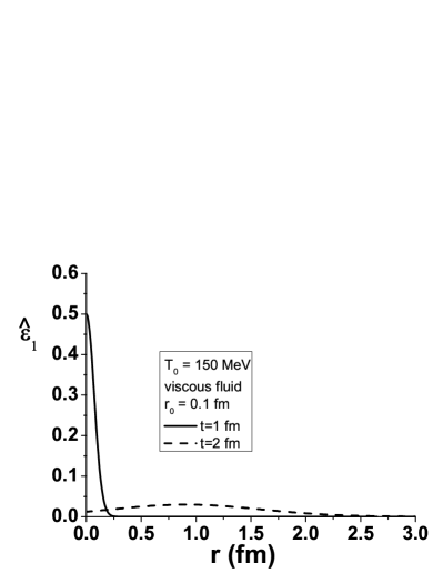
(b)

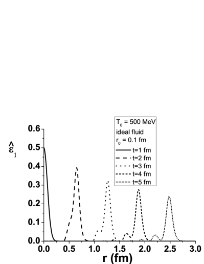
(c)

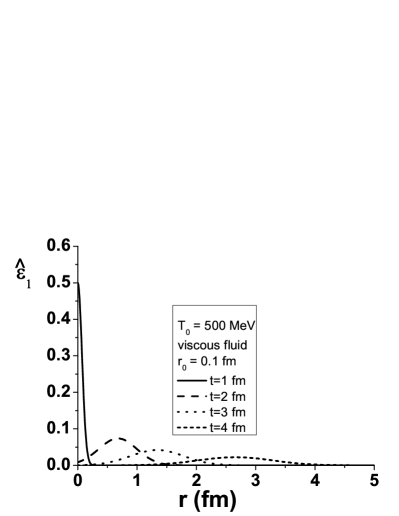
(d)

Figure 2: Numerical solutions of (60) for an ideal fluid (left) and of (61) for a viscous fluid (right). The solutions are for several times and for $T_{0}=150$ MeV (upper panels) and $T_{0}=500$ MeV (lower panels). The initial amplitude is $0.5$ and the width $r_{0}=0.1\,\,fm$.

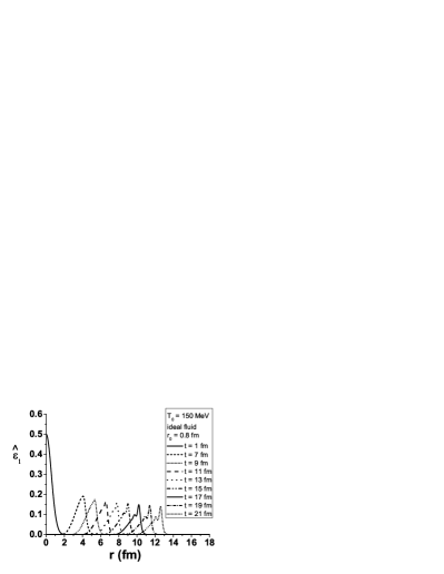
(a)

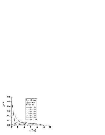
(b)

(c)

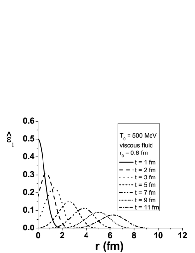
(d)

Figure 3: Numerical solutions of (60) for an ideal fluid (left) and of (61) for a viscous fluid (right). The solutions are for several times and for $T_{0}=150$ MeV (upper panels) and $T_{0}=500$ MeV (lower panels). The initial amplitudes $0.5$ and the width is $r_{0}=0.8\,\,fm$.

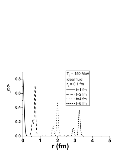
(a)

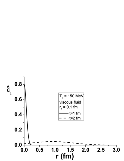
(b)

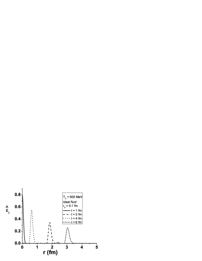
(c)

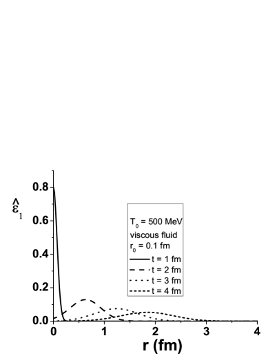
(d)

Figure 4: Numerical solutions of (60) for an ideal fluid (left) and of (61) for a viscous fluid (right). The solutions are for several times and for $T_{0}=150$ MeV (upper panels) and $T_{0}=500$ MeV (lower panels). The initial amplitude is $0.8$ and the width is $r_{0}=0.1\,\,fm$.

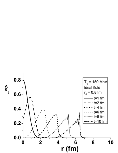
(a)

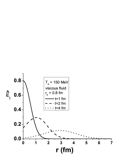
(b)

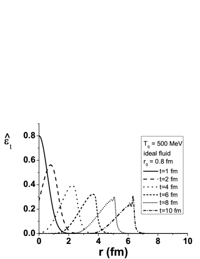
(c)

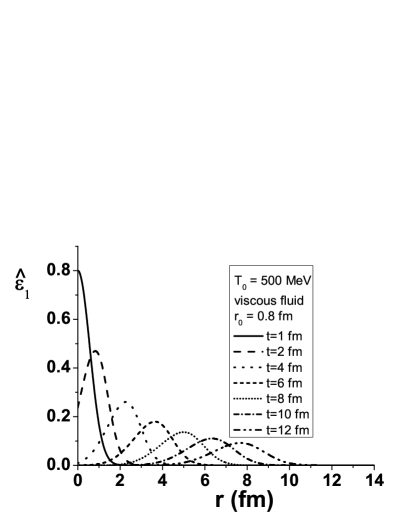
(d)

Figure 5: Numerical solutions of (60) for an ideal fluid (left) and of (61) for a viscous fluid (right). The solutions are for several times and for $T_{0}=150$ MeV (upper panels) and $T_{0}=500$ MeV (lower panels). The initial amplitude is $0.8$ and the width is $r_{0}=0.8\,\,fm$.

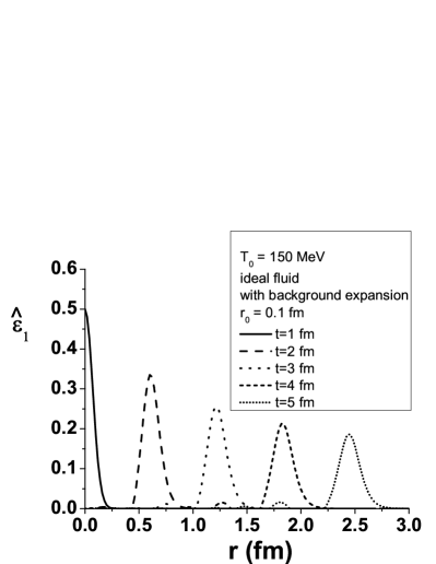
(a)

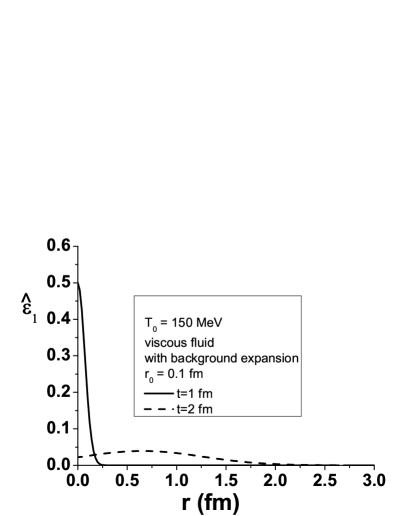
(b)

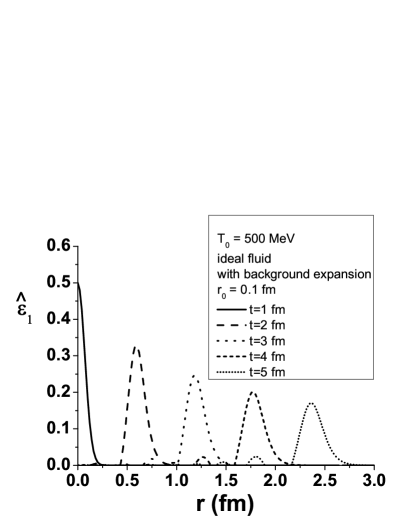
(c)

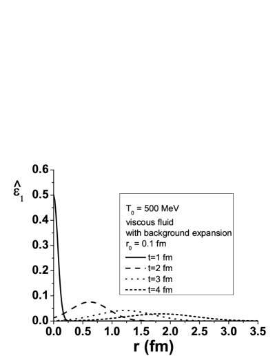
(d)

Figure 6: The same as of Fig. 2 with background fluid expansion. The curves show numerical solutions of (60) and (61) with a changing $T_{0}$, given by Eq. (55).

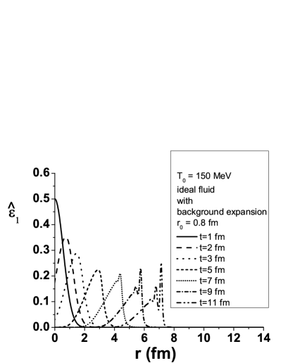
(a)

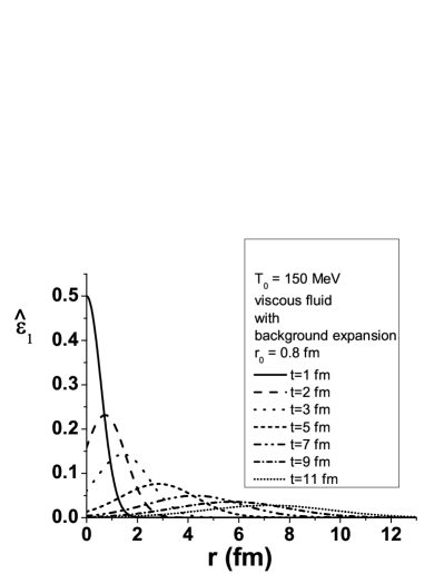
(b)

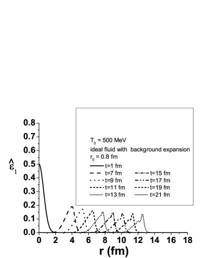
(c)

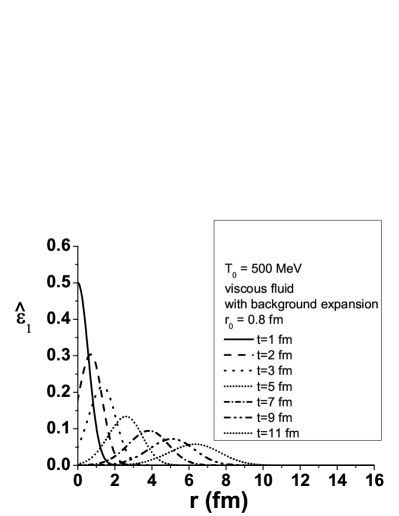
(d)

Figure 7: The same as of Fig. 3 with background fluid expansion. The curves show numerical solutions of (60) and (61) with a changing $T_{0}$, given by Eq. (55).

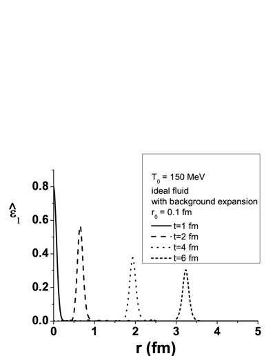
(a)

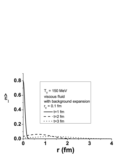
(b)

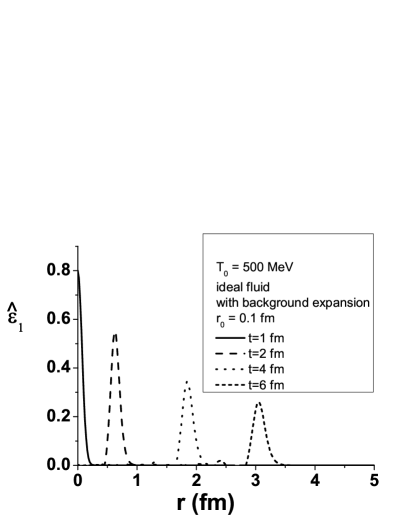
(c)

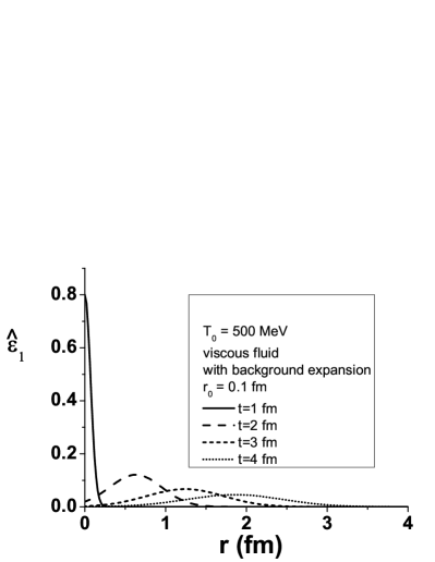
(d)

Figure 8: The same as of Fig. 4 with background fluid expansion. The curves show numerical solutions of (60) and (61) with a changing $T_{0}$, given by Eq. (55).

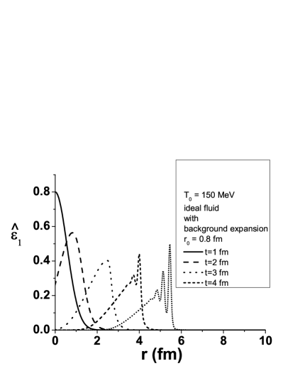
(a)

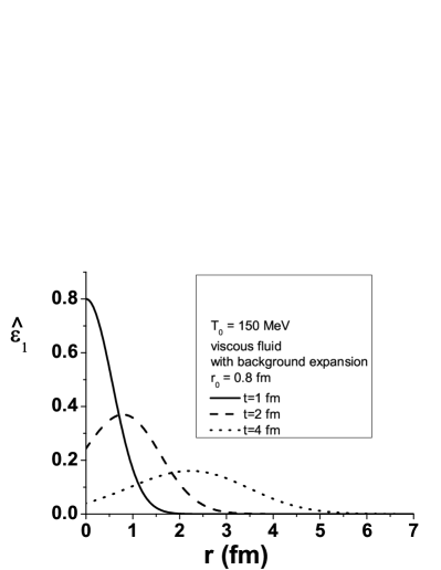
(b)

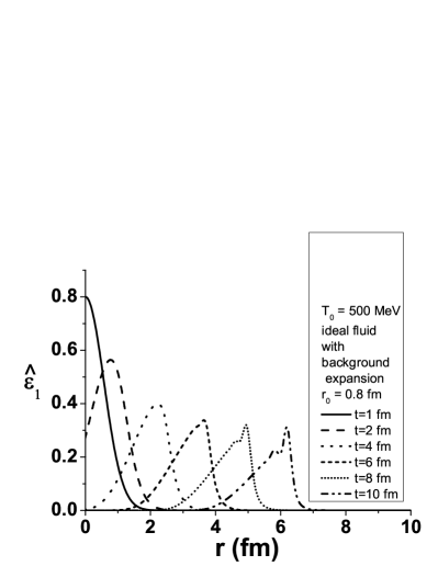
(c)

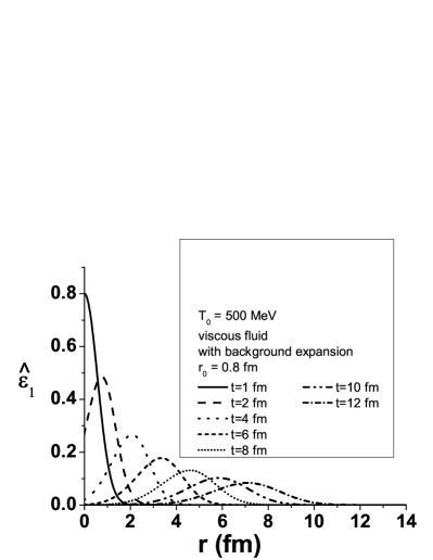
(d)

Figure 9: The same as of Fig. 5 with background fluid expansion. The curves show numerical solutions of (60) and (61) with a changing $T_{0}$, given by Eq. (55).

In the numerical analysis there are many cases to be considered. We present our results in eight figures (Figs. 2 - 9). The first four refer to the static background and the second group of four shows solutions for the same parameters for the case of an expanding background. All figures have four panels. The two upper panels refer to the low temperature ($T_{0}=150$ MeV) and the two lower panels to the high temperature ($T_{0}=500$ MeV). The two panels on the left show results with the ideal fluid and the two panels on the right results with the viscous fluid. From the figures we want to see how sensitive the expansion of the tube is to changes in: i) the initial amplitude, ii) the temperature, iii) the tube radius, iv) the strength of viscosity and v) the expansion of the background fluid. In what follows we discuss the role played by each one of these variables mentioning them by order of relevance.

V.0.1 Viscosity

The most striking finding is the strong influence of viscosity. This can be seen in all figures and most clearly in the comparison between Fig. 2a) and 2b). Viscosity damps the amplitude of the pulse by a factor ten in 1 fm! Increasing the temperature of the medium reduces the effect of viscosity as it can be seen from the factor $1/T_{0}$ in (61). However the comparison between Fig. 2b) and 2d) shows that this reduction is not very strong. The role played by viscosity is also reduced when the initial radius parameter of the tube goes from $r_{0}=0.1$ to $0.8$ fm. This is easy to understand looking at (62) and then at the right hand side of (61). A broader initial distribution generates smaller spatial gradients appearing in the viscosity term of (61), which becomes smaller. Nevertheless the attenuation of the initial pulse remains strong as compared to the ideal fluid case. This situation is illustrated in Fig. 3, which is to be compared with Fig. 2. If we increase the initial amplitude from $A=0.5$ to $A=0.8$, the relevance of viscosity remains the same. This can be checked by comparing Fig. 2 with Fig. 4 and also comparing Fig. 3 with Fig. 5. The introduction of the background cooling preserves the difference between ideal and viscous fluids, as can be inferred from the comparison between Figs. 2, 3, 4, 5 and their analogues with cooling Figs. 6, 7, 8 and 9.

The introduction of viscosity in our calculations is what more strongly changes them. As anticipated in the introduction, due to dissipation, viscosity strongly damps and broadens the tubes during their expansion and they are more easily mixed with the background fluid, loosing their influence on final state particle correlations. This is a robust conclusion of our numerical analysis since it remains valid in all situations considered. Moreover viscosity prevents the perturbation wave from breaking, as can be seen comparing, for example, Fig. 5a) with 5b) or comparing Fig. 7a) with 7b). Looking at the time evolution of the peaks of the pulses, we can have an idea of the velocity with which they propagate. Comparing the left with right side of all figures we can see the velocity of the pulses is only weakly changed by viscosity. This velocity is defined by the sound velocity, which in our approach is the same both for ideal and viscous fluids.

V.0.2 Initial radius of the tube

The solutions of nonlinear differential equations, such as (60) and (61), are expected to depend on the initial condition. We can check this dependence changing the parameters in (62) and solving again both (60) and (61). The comparison between Fig. 2 with Fig. 3 and also the comparison between Fig. 4 with Fig. 5 shows that, after viscosity, changes in the initial tube radius are those which most substantially affect the tube evolution. Essentially thinner tube are more fragile. They break more easily, developing secondary bumps (called “radiation”) and/or forming a wall with rapid oscillations at the edge. These instabilities may lead to loss of localization and absorption of the tube by the medium. Larger tubes, on the other hand, live longer in the plasma. This conclusion may be relevant for the physics of particle correlation studied now at RHIC and LHC. Moreover, the transverse size of the tubes has physical origins. Glasma flux tubes are typically thinner raju12 than the tubes obtained in event generator based on string models (see hamatube and andrade for details).

V.0.3 Initial amplitude of the tube

Figs. 4 and 5 are repetitions of 2 and 3 with a larger amplitude. These cases are very interesting for us because in perturbations with larger amplitudes the nonlinear effects become more important. The reductive perturbation method (RPM) employed here is well suited to preserve the nonlinearities of the original equations and transfer them to the equations which govern the evolution of perturbations. From the figures we can conclude that pulses with larger amplitudes break faster. However the effect is not very pronounced because the range of variation considered here is relatively narrow: $0.5<A<0.8$.

V.0.4 Temperature

Comparing in all figures the upper panels with the lower panels, we conclude that, in the case of ideal fluids, there are only small differences between them. This weak dependence on the temperature might have been anticipated from a closer look at the coefficient of the nonlinear term in (60) and in (61). The temperature dependent term in this coefficient can vary only between zero and one, changing the overall coefficient at most by a factor two (in realistic calculations the range of variation is even narrower because of the limits in the temperature: $150<T_{0}<500$ MeV). This weak sensitivity comes from all the developments which led to (60) and is difficult to say what is more responsible for the final result, whether the equation of state or the approximations adopted. In contrast, the temperature dependence of the viscosity term in Eq. (61) is slightly stronger. Therefore the comparison of upper with lower panels on right side of all figures reveals more pronounced differences. In viscous fluids the increase of temperature decreases the amplitude of the pulse and makes it live longer. The second derivative term in the Burgers equations does not permit the breaking and dispersion of the pulse. However, together with the geometrical term $\hat{\varepsilon}_{1}/2t$, it causes the attenuation of the tube. In our calculations the viscosity coefficients ($\eta$ and $\zeta$) were kept constant but they may be temperature dependent, enhancing the sensitivity of our results to the temperature.

V.0.5 Background expansion

We have repeated all the calculations replacing (52) and (54) by (58) and (59). The numerical solution of the latter equations (neglecting the derivatives with respect to $z$) is presented in Figs. 6 to 9. The effect of the Bjorken cooling is to slightly reduce the amplitude of the pulse, which can be best seen comparing Fig. 2 with Fig. 6 and Fig. 3 with Fig. 7. It is a small effect and this is very interesting. The cooling studied here is a crude representation of the real three dimensional background fluid expansion. If we had found that cooling is important, this would suggest that a realistic treatment of the background expansion would change completely the conclusions obtained so far. This seems not to be the case.

V.1 Final remarks

If, on one hand, the similarity between the figures is somewhat deceptive (because of the weak dependence on the dynamical ingredients), on the other hand they deliver a strong message: the tube expands radially with a supersonic velocity and in less than 4 fm/c it becomes a “ring”, with a hole in the middle. Moreover, by this time the amplitude is already reduced by a factor two and the tube (or ring) looses the strength to “push away” the surrounding matter. This agrees with the results found in andrade , where the evolution of a tube was studied in a different way. In that work the numerical solution of the hydrodynamical equations of the total system (tubular perturbation + background) was obtained, whereas here we have isolated the perturbation from the background and written a differential equation for it. We have provided an independent check of the results found in andrade with the use of a different equation of state.

An important conclusion of our work is that viscosity strongly affects the propagation of perturbations in the quark gluon plasma. This conclusion was obtained with the relativistic Navier-Stokes formalism and it would be interesting to check if it remains valid in other relativistic theories of viscosity.

VI Appendix

The derivation of Eq. (54) is quite similar to derivation of Eq. (52) and here we would like to add some details. The expansion of Eqs. (16) and (18) in powers of $\sigma$ is straightforward. The calculation is faster if we keep terms only up to $\sigma^{2}$ and neglect some higher order terms even before reaching the identities equivalent to (40), (41) and (42). It is useful to remember that:

$$\gamma^{n}\cong 1+(n/2)\times v^{2}\hskip 5.69046pt\propto\hskip 5.69046pt1+\sigma^{2}+\dots$$

$${\frac{\partial\gamma}{\partial t}}=\gamma^{3}v{\frac{\partial v}{\partial t}}\hskip 8.5359pt\propto\hskip 8.5359pt\sigma^{5/2}\hskip 25.6073pt\textrm{and}\hskip 25.6073pt\vec{\nabla}\gamma=\gamma^{3}v\vec{\nabla}v\hskip 8.5359pt\propto\hskip 8.5359pt\sigma^{5/2}$$ (63)

The viscous terms in (16) are of the following order in $\sigma$:

$$\eta\,v^{i}\partial_{\mu}\partial^{\mu}\gamma\hskip 8.5359pt\propto\hskip 8.5359pt\sigma^{4}$$ (64)

$$\eta\,v^{i}\partial_{\mu}{\frac{\partial u^{\mu}}{\partial t}}\hskip 8.5359pt\propto\hskip 8.5359pt\sigma^{3}$$ (65)

$$\eta\,v^{i}\partial_{\mu}\bigg{[}\gamma\bigg{(}{\frac{\partial}{\partial t}}+\vec{v}\cdot\vec{\nabla}\bigg{)}(\gamma u^{\mu})\bigg{]}\bigg{\}}\hskip 8.5359pt\propto\hskip 8.5359pt\sigma^{3}$$ (66)

$$v^{i}\bigg{(}\zeta-{\frac{2}{3}}\eta\bigg{)}{\frac{\partial}{\partial t}}\bigg{[}{\frac{\partial\gamma}{\partial t}}+\vec{\nabla}\cdot(\gamma\vec{v})\bigg{]}\hskip 8.5359pt\propto\hskip 8.5359pt\sigma^{3}$$ (67)

$$+v^{i}\bigg{(}\zeta-{\frac{2}{3}}\eta\bigg{)}\partial_{\mu}\bigg{\{}\gamma u^{\mu}\bigg{[}{\frac{\partial\gamma}{\partial t}}+\vec{\nabla}\cdot(\gamma\vec{v})\bigg{]}\bigg{\}}\hskip 8.5359pt\propto\hskip 8.5359pt\sigma^{3}$$ (68)

$$\eta\,\partial_{\mu}\partial^{\mu}(\gamma v^{i})\hskip 8.5359pt\propto\hskip 8.5359pt\sigma^{2}$$

$$\eta\,\partial_{\mu}\partial^{i}u^{\mu}\hskip 8.5359pt\propto\hskip 8.5359pt\sigma^{2}$$

$$\eta\,\partial_{\mu}\bigg{[}\gamma\bigg{(}{\frac{\partial}{\partial t}}+\vec{v}\cdot\vec{\nabla}\bigg{)}(\gamma v^{i}u^{\mu})\bigg{]}\bigg{\}}\hskip 8.5359pt\propto\hskip 8.5359pt\sigma^{2}$$

$$\bigg{(}\zeta-{\frac{2}{3}}\eta\bigg{)}\partial^{i}\bigg{[}{\frac{\partial\gamma}{\partial t}}+\vec{\nabla}\cdot(\gamma\vec{v})\bigg{]}\hskip 8.5359pt\propto\hskip 8.5359pt\sigma^{2}$$

$$\bigg{(}\zeta-{\frac{2}{3}}\eta\bigg{)}\partial_{\mu}\bigg{\{}\gamma v^{i}u^{\mu}\bigg{[}{\frac{\partial\gamma}{\partial t}}+\vec{\nabla}\cdot(\gamma\vec{v})\bigg{]}\bigg{\}}\hskip 8.5359pt\propto\hskip 8.5359pt\sigma^{3}$$ (69)

Using (64) to (69) in (16) and keeping only terms up to $\mathcal{O}(\sigma^{2})$ we obtain:

$$(\varepsilon+p)\gamma^{2}\bigg{(}{\frac{\partial}{\partial t}}+\vec{v}\cdot\vec{\nabla}\bigg{)}v^{i}+v^{i}{\frac{\partial p}{\partial t}}-\partial^{i}p$$

$$+\eta\,\bigg{[}\gamma\,\bigg{(}{\frac{\partial^{2}v^{i}}{\partial t^{2}}}-\vec{\nabla}^{2}v^{i}\bigg{)}+\gamma\,\partial^{i}(\vec{\nabla}\cdot\vec{v})-\gamma^{3}\,{\frac{\partial^{2}v^{i}}{\partial t^{2}}}\bigg{]}+\bigg{(}\zeta-{\frac{2}{3}}\eta\bigg{)}\gamma\,\partial^{i}(\vec{\nabla}\cdot\vec{v})=0$$ (70)

The $\gamma^{n}$ (with $n=1,2,3$) factors in (70) are also multiplying $v^{i}$ or its derivative, which contributes with at least one power of $\sigma$. Therefore we consider $\gamma^{n}\cong 1$ and (70) becomes:

$${\frac{\partial\vec{v}}{\partial t}}+(\vec{v}\cdot\vec{\nabla})\vec{v}=-{\frac{1}{(\varepsilon+p)}}\bigg{[}\vec{\nabla}p+\vec{v}{\frac{\partial p}{\partial t}}\bigg{]}+{\frac{1}{(\varepsilon+p)}}\bigg{[}\eta\,{\vec{\nabla}}^{2}\vec{v}+\bigg{(}\zeta+{\frac{1}{3}}\eta\bigg{)}\vec{\nabla}(\vec{\nabla}\cdot\vec{v})\bigg{]}$$ (71)

The equation above is the simplified version of the relativistic Navier-Stokes equation and from (71) it is easier to derive (53).

Analogously we estimate the order (in $\sigma$) of the viscous terms in (18):

$${\frac{\eta}{T}}\bigg{(}{\frac{\partial\gamma}{\partial t}}\bigg{)}^{2}\propto\hskip 8.5359pt\sigma^{5}$$ (72)

$${\frac{\eta}{T}}\bigg{[}\vec{\nabla}\gamma\cdot{\frac{\partial}{\partial t}}(\gamma\vec{v})\bigg{]}\hskip 8.5359pt\sigma^{4}$$ (73)

$${\frac{\eta}{T}}(\partial^{i}u^{j})\partial_{j}u_{i}\propto\hskip 8.5359pt\sigma^{3}$$ (74)

$${\frac{1}{T}}\bigg{(}{\frac{2}{3}}\eta+\zeta\bigg{)}\,\bigg{[}{\frac{\partial\gamma}{\partial t}}+\gamma\vec{\nabla}\cdot\vec{v}+\vec{\nabla}\gamma\cdot\vec{v}\bigg{]}^{2}\propto\hskip 8.5359pt\sigma^{3}$$ (75)

(a)

- (1) F. Gelis, arXiv:1110.1544 [hep-ph].
- (2) K. Fukushima and F. Gelis, arXiv:1106.1396 [hep-ph].
- (3) T. Lappi and L. McLerran, Nucl. Phys. A 772, 200 (2006).
- (4) A. Dumitru, F. Gelis, L. McLerran and R. Venugopalan, Nucl. Phys. A 810, 91 (2008).
- (5) Y. Hama, R.P.G. Andrade, F. Grassi, W. -L. Qian, Nonlin. Phenom. Complex Syst. 12 , 466 (2009); R.P.G. Andrade, F. Grassi, Y. Hama and W.-L. Qian, arXiv:1012.5275 [hep-ph]; J. Phys. G G 37, 094043 (2010); R.P.G. Andrade, F. Gardim, F. Grassi, Y. Hama and W.L. Qian, J. Phys. G 38, 124123 (2011).
- (6) R.P.G. Andrade, F. Grassi, Y. Hama and W.L. Qian, Nucl. Phys. A 854, 81 (2011); arXiv:1008.4612 [nucl-th].
- (7) P. Staig and E. Shuryak, arXiv:1109.6633 [nucl-th].
- (8) P. Staig and E. Shuryak, Phys. Rev. C 84, 044912 (2011); Phys. Rev. C 84, 034908 (2011); arXiv:1106.3243.
- (9) D. A. Fogaça, L. G. Ferreira Filho and F. S. Navarra, Phys. Rev. C 81, 055211 (2010).
- (10) D. A. Fogaca, F. S. Navarra and L. G. Ferreira Filho, Phys. Rev. D 84, 054011 (2011).
- (11) P. Romatschke, Int. J. Mod. Phys. E 19, 1 (2010).
- (12) S. Weinberg,“Gravitation and Cosmology”, New York: Wiley, 1972.
- (13) L. Landau and E. Lifchitz, “Fluid Mechanics”, Pergamon Press, Oxford, (1987).
- (14) R. C. Davidson, “Methods in Nonlinear Plasma Theory”, Academic Press, New York an London, 1972, pages 20 and 21.
- (15) D.A. Fogaça and F.S. Navarra, Phys. Lett. B 639, 629 (2006).
- (16) D.A. Fogaça and F.S. Navarra, Phys. Lett. B 645, 408 (2007).
- (17) D.A. Fogaça and F.S. Navarra, Nucl. Phys. A 790, 619c (2007); Int. J. Mod. Phys. E 16, 3019 (2007).
- (18) D.A. Fogaça, L. G. Ferreira Filho and F.S. Navarra, Nucl. Phys. A 819, 150 (2009).
- (19) W.M. Moslem, U.M. Abdelsalam, R. Sabry, E.F.El-Shamy and S.K. El-Labany, J. Plasma Phys. 76, 453 (2010).
- (20) A. Jeffrey, T. Kawahara, “Asymptotic Methods in Nonlinear Wave Theory”, Pitman, Boston, (1981).
- (21) R. K. Dodd, J. C. Eilbeck, J. D. Gibbon and H. C. Morries, “Solitons and Nonlinear Wave Equations”, Academic Press Inc., (1982).
- (22) See, for example, A.K. Chaudhuri, arXiv:1111.5713 [nucl-th] and also Victor Roy and A.K. Chaudhuri, arXiv:1201.4230v1 [nucl-th].
- (23) B. Schenke, P. Tribedy and R. Venugopalan, arXiv:1202.6646 [nucl-th].
- (24) J.D. Bjorken, Phys.Rev. D 27, 140 (1983).
- (25) A. A. Mamun and P. K. Shukla, Europhys. Lett. 87, 25001 (2009); A. A. Mamun and P. K. Shukla, Europhys. Lett. 94, 65002 (2011).
- (26) B. Sahu, Bulg. J. Phys. 38, 175 (2011).