Hadron-quark phase transition in a hadronic and Polyakov–Nambu–Jona-Lasinio models perspective

Abstract

In this work we study the hadron-quark phase transition matching relativistic hadrodynamical mean-field models (in the hadronic phase) with the more updated versions of the Polyakov-Nambu-Jona-Lasinio models (on the quark side). Systematic comparisons are performed showing that the predicted hadronic phases of the matching named as RMF-PNJL, are larger than the confined phase obtained exclusively by the Polyakov quark models. This important result is due to the effect of the nuclear force that causes more resistance of hadronic matter to isothermal compressions. For sake of comparison, we also obtain the matchings of the hadronic models with the MIT bag model, named as RMF-MIT, showing that it presents always larger hadron regions, while shows smaller mixed phases than that obtained from the RMF-PNJL ones. Thus, studies of the confinement transition in nuclear matter, done only with quark models, still need nuclear degrees of freedom to be more reliable in the whole $T\times\mu$ phase diagram.

I Introduction

The study of the properties of the strongly interacting matter is experimentally supported by the heavy-ion collisions at ultrarelativistic energies, accomplished in the most sophisticated accelerators such as the relativistic heavy-ion collider (RHIC) and the large hadron collider (LHC). The measurements coming from these experiments are indirectly used to furnish the basic information on the phase diagram concerning the state of matter, being the different regions related to the distinct hadronic (confined quarks), and the quark-gluon plasma (free quarks) phases. In order to cover the temperature-density/chemical potential plane of the hadron-quark phase diagram, the new experiments should be able to compress the baryonic matter even to higher densities compared to the well known nuclear saturation density, $\rho_{0}\approx 0.16$ fm^-3. The new facility for antiproton and ion research (FAIR) fair at Darmstadt, and the nuclotron-based ion collider facility (NICA) nica at the Joint Institute for Nuclear Research (JINR) in Dubna, will make possible such extreme conditions through collisions foreseen to reach an energy range of $8$ to $45$ $A$ GeV fair . Therefore, it will be possible to test the predictions from the theoretical calculations about the order of hadron-quark phase transition (crossover, first order or both), and also the regime of high density and moderate temperatures.

On the theoretical side, the strongly interacting matter is described by Quantum Chromodynamics (QCD). In its nonperturbative regime of large distances, or equivalently low energies, the most important method to study the QCD structure is the numerical lattice calculations lattice , with the Monte Carlo simulations mcarlo being its mainly representative. Such techniques provide results as for the pure gluon sector, i.e., in the limit of infinitely heavy quarks, as for systems including dynamical quarks. The difficulties in the latter are in the fact that at finite quark chemical potential ($\mu_{q}$) regime, the numerical calculations face to the fermion sign problem sign . However, alternatives to solve this question are addressed in many methods expansao ; reweighting ; review ; imaginary ; dos . On the other hand, one can deal with the high energy QCD regime (asymptotically free region) freeqcd in a complete theoretical way through the perturbative treatment.

To investigate the moderate and high density regime of the transition, it is needed effective models such as the MIT bag model mit and the Nambu-Jona-Lasinio (NJL) njl ; buballa ; outros one, that curiously were firstly proposed to describe the hadronic mass spectrum. The former treats gluons and massless quarks as free particles in which the confinement phenomenon is incorporated by including a bag constant in an ad hoc fashion. The latter presents further similarities with the full QCD theory but do not take into account the confinement, since the quarks interact each other via pointlike interactions with no mediator gluons. One of the mainly aims of these kind of models is to provide the QCD phase diagram in the $T\times\mu$ plane in order to distinguish hadronic phase where the chiral symmetry is broken, and the quark one. The quark stars description with these effective models is in the same important way buballa ; stocker1 .

The phenomenology of the hadron-quark phase transition is often studied with the mentioned effective QCD models astroj ; wang and other. Recently, a study about the QCD phase diagram was accomplished in Ref. kapusta where the linear $\sigma$ model was used to construct the phase transition curve, in the two-flavor quark system, as a function of the vacuum pion mass. It was shown that the point in the $T\times\mu$ plane where is changed the phase transition order, the critical end point, is sensitive to this parameter. In such cases, where there is only one model (the quark one), the identified phases in the transition curve are associated to those with broken and restored chiral symmetry.

To distinguish hadron and quark phases we have the following well accepted phenomenology. The strongly interacting matter at very high temperatures and baryon densities should have quarks and gluons as the degrees of freedom. Motivated QCD models, cited above mit ; njl ; buballa ; outros take these degrees of freedom into account. On the other side, at low temperatures ($T<20$ MeV) and moderate densities of the order of $\rho_{0}$, the hadronic phase can not be described by quarks and gluons. Instead, nucleons and mesons are the relevant degrees of freedom. Here, different approaches as Brueckner-Hartree-Fock by using realistic two-nucleon interactions bhf , or relativistic mean-field (RMF) models may describe quite well the nuclear matter and finite nuclei properties. Between these two phases a mixed region takes place.

In this work, we focus in two structurally distinct models to treat the hadron-quark phase transition, namely, the Polyakov Nambu-Jona-Lasinio (PNJL) models in the characterization of the quark phase, and the relativistic mean-field nonlinear Walecka ones in the description of the phase where the chiral symmetry is broken, i.e., the hadronic phase. The former is a generalization of the NJL model in the sense that the confinement phenomenon is incorporated in its structure. For sake of comparison, we also perform a hadron-quark phase transition using the MIT Bag model in the quark side, in order to see explicitly the effect of the dynamical confinement contained in the PNJL model compared with the MIT Bag one.

The motivation for such an approach matching two models with different degrees of freedom is the following. MIT bag and PNJL models do not describe any of the very well known properties of the ordinary nuclear matter while attempting only to achieve, through phase diagrams, the boundaries where this matter starts to be confined. In this aspect only with such models a more complete description is poor. On the other side, the RMF models constructed to well describe the bulk nuclear matter and finite nuclei properties, are often applied to investigate high density regimes as it is common for neutron stars. Whether in such regions the RMF models are still valid is questionable. The phase transition between the quark and the hadron phase helps understanding when one needs to start describing nuclear matter with other degrees of freedom than baryons and mesons employed by RMF models. Therefore, our study brings more information for the mixed phase between these two still disconnected quark and hadronic phases. The use of different PNJL and RMF models is needed if one wants to have a more precise conclusion about how the different families of hadronic and quark models predict mixed phases. If they are similar or not, or still whether the description of the confined/deconfined phase transition only via the PNJL model itself is totally trustable when compared with the approach matching the two models. As we will show, this phase transition obtained by only the PNJL model, is expected to occur in a much smaller chemical potential for the same temperature differing strongly of the transition obtained by RMF-PNJL models. Future experiments, discussed already before, will show what description is correct.

After the first version of this manuscript was submitted, we became aware of a very similar study in which the hadron-quark phase transition was investigated only with one parametrization for the PNJL and RMF model gyshao . Our systematic study here goes beyond that work, in the following aspects. Our calculations will take into account here different parametrizations for both, the PNJL and RMF models. In the latter, we will analyze a class of hard and soft equations of state, in a very large range of the nuclear matter incompressibility, $172<K<554$ MeV, and show that, actually, the RMF models affect quite small the entire hadron-quark phase transition. In the former, the most up to date Polyakov potential parametrizations will be used and compared each other. Still, a comparative study involving the hadron-quark phase transition with the MIT bag model will be performed.

This paper is organized as follows. In Sec. II, we present the quark models used in this work, starting by the MIT Bag model and later with the PNJL one, where a comparison between the current parametrizations, regarding their thermodynamics, is also done. In Sec. III, the mainly features of the RMF models are presented, and in Sec. IV, the phase diagrams concerning the hadron-quark phase transitions are shown. Our summary and conclusions are in the last section.

II Quark models

II.1 MIT Bag model

Possibly, the simplest model to describe an approximate physics describing the matter where quark and gluons are the proper degrees of freedom of the system is the MIT bag model mit . Such a scenario is supposed to exist at very high density or temperature regimes. Back in the big bang theory, at the very beginning, the universe was very hot and dense before hadronization. Nowadays, very high energy heavy-ion collision experiments in LHC try to recreate the signatures to confirm this hypothesis. In the case it is confirmed, hot hadronic matter undergoes a phase transition to the quark-gluon plasma (QGP) at uncertain but very high and very low temperature and density, respectively. The phase diagram connecting the QGP phase to a pure hadronic phase from high to zero temperature is still a big challenge and has a model dependence exhibited in previous studies when some relativistic hadronic models and the MIT bag ones were investigated jphysg ; debora . The MIT bag model itself does not describe the confined hadronic phase but rather the QGP. Therefore, the hadronic phase has to be represented by any hadronic model in which the degree of freedom are baryons and mesons as we will present later on. Once each phase is modeled, the phase diagram is obtained thermodynamically by the Gibbs criteria, matching the chemical potential and the pressure at a given temperature ($T_{c}$), across the phase boundaries when a phase transition takes place. Explicitly, these criteria are

$$\mu_{H}(T_{c},\rho^{c}_{H}) = \mu_{QGP}(T_{c},\rho^{c}_{QGP})$$ (1)

$$P_{H}(T_{c},\rho^{c}_{H}) = P_{QGP}(T_{c},\rho^{c}_{QGP}).$$ (2)

As previously presented jphysg , the set of critical $\rho^{c}$’s establishes curves $\rho^{c}(T)$ in the $(\rho,T)$ plane. Below the $(\rho^{c}_{H},T_{c})$ curve the system may be interpreted as nuclear matter described by the hadronic models (hadronic sector). The region in between $(\rho^{c}_{H},T_{c})$ and $(\rho^{c}_{QGP},T_{c})$ corresponds to a mixed (H-QGP) coexistence phase. Above the $(\rho^{c}_{QGP},T_{c})$ curve, the system is in a pure QGP phase.

For the quark-gluon plasma phase in the MIT bag model, the pressure and baryon number density are given by heinz ; boqiang

$$P_{\mbox{\tiny MIT}}(\mu_{q},T_{q}) = \frac{8\pi^{2}T_{q}^{4}}{45}\left(1-\frac{15\alpha_{s}}{4\pi}\right)+N_{f}\left[\frac{7\pi^{2}T_{q}^{4}}{60}\left(1-\frac{50\alpha_{s}}{21\pi}\right)\right.$$ (3)

$$+ \left.\left(\frac{\mu_{q}^{2}T_{q}^{2}}{2}+\frac{\mu_{q}^{4}}{4\pi^{2}}\right)\left(1-\frac{2\alpha_{s}}{\pi}\right)\right]-B,\,\qquad\mbox{and}$$

$$\rho_{\mbox{\tiny MIT}} = \frac{1}{3}N_{f}\left(\mu_{q}T_{q}^{2}+\frac{\mu_{q}^{3}}{\pi^{2}}\right)\left(1-\frac{2\alpha_{s}}{\pi}\right),$$ (4)

where $B$ is the bag constant, $N_{f}$ is the number of flavors and $\alpha_{s}$ is the QCD running coupling constant, depending on the quark-gluon plasma temperature $T_{q}$ and the quark chemical potential $\mu_{q}$ through the first order perturbative expression

$$\alpha_{s}=4\pi\left\{\left(11-\frac{2N_{f}}{3}\right)\ln[\left(0.8\mu_{q}^{2}+15.622T_{q}^{2}\right)/\Lambda^{2}]\right\}^{-1}\,.$$ (5)

In this paper, the MIT bag model will be used only as a comparison with the PNJL model, regarding the predictions for the boundaries of the hadronic and QGP phases for each specific RMF model describing the hadronic phase.

II.2 PNJL model

II.2.1 Confinement

The confinement can be measured by the Polyakov loop, defined as a Wilson line in the Euclidean space-time by $L=\mathcal{P}$exp$(i\int_{0}^{\beta}d\tau A_{4})$ where $A_{4}$ is the gauge field. By this definition, it can be viewed as a closed path connecting the same point in the space, at the different times $0$ and $\beta=1/T$. The traced Polyakov loop, $\Phi=\mbox{Tr}_{c}(L)/N_{c}$ with $N_{c}$ being the quark color number, plays an important role concerning the deconfinement since it is the order parameter of this transition. Actually, the deconfinement is a consequence of the global center symmetry breaking. In pure gauge systems at finite temperature, where the periodic boundary conditions are satisfied, this symmetry is realized by the gauge transformations due to the way how they affect the boson fields. The consequence in the traced Polyakov loop is that $\Phi\rightarrow e^{\frac{2\pi ik}{N_{c}}}\Phi$, with $k=1,2,3...$ what means that the condition $\Phi=0$ has to be fulfilled in order to keep the center symmetry preserved. Since $\Phi$ is related with free energy of a color source, through $\Phi=e^{-F_{q}/k_{B}T}$, if the center symmetry is realized, then $F_{q}\rightarrow\infty$, meaning that the quark is confined. In dynamical quark systems where the fermionic field explicitly breaks the center symmetry, generating automatically $\Phi\neq 0$, the traced Polyakov loop is considered as an approximated deconfinement order parameter. The situation is analog to the cases in which the system Lagrangian density presents a mass term that explicitly breaks the chiral symmetry. The condensate $\left<\bar{\psi}_{q}\psi_{q}\right>$ is also an approximated order parameter, in this case for the restored chiral symmetry phase. The confinement effect, associated with $\Phi$, was implemented originally in the NJL model by Fukushima fuku1 and deeply studied in Refs. weise1 ; weise2 ; weise3 ; weise4 ; weise5 ; weise6 ; weise7 . The PNJL model is able to describe as the broken-unbroken chiral symmetry as the confinement-deconfinement phase transitions even being this situations, respectively, in the opposite regimes of vanishing and infinite quark masses fuku1 .

II.2.2 Thermodynamical calculations at $T\neq 0$

The connection between the fermion and the gauge field in the PNJL model is done by making the substitution $\partial^{\mu}\rightarrow\partial^{\mu}+iA^{\mu}$ in the Lagrangian density. The after bosonization of the system, and the mean-field approximation lead to the following grand canonical potential per volume weise2 :

$$\Omega_{\mbox{\tiny PNJL}} = \mathcal{U}(\Phi,\Phi^{*},T)+\frac{G{\rho_{sq}}^{2}}{2}-\frac{\gamma_{q}}{2\pi^{2}}\int_{0}^{\Lambda}E_{q}\,k^{2}dk$$ (6)

$$- \frac{\gamma_{q}T}{2\pi^{2}N_{c}}\int_{0}^{\infty}\mbox{ln}\left[1+3\Phi e^{-(E_{q}-\mu_{q})/T}+3\Phi^{*}e^{-2(E_{q}-\mu_{q})/T}+e^{-3(E_{q}-\mu_{q})/T}\right]k^{2}dk$$

$$- \frac{\gamma_{q}T}{2\pi^{2}N_{c}}\int_{0}^{\infty}\mbox{ln}\left[1+3\Phi^{*}e^{-(E_{q}+\mu_{q})/T}+3\Phi e^{-2(E_{q}+\mu_{q})/T}+e^{-3(E_{q}+\mu_{q})/T}\right]k^{2}dk,$$

being $\,E_{q}=(k^{2}+{M_{q}}^{2})^{1/2}\,$, $\,\rho_{sq}=\left<\bar{\psi_{q}}\psi_{q}\right>=\left<\bar{u}u\right>+\left<\bar{d}d\right>=2\left<\bar{u}u\right>\,$ in the isospin symmetric system, $\,\mathcal{U}(\Phi,\Phi^{*},T)\,$ the effective Polyakov loop potential in terms of $\Phi$ and its conjugate $\Phi^{*}$, that we will discuss later, and $\gamma_{q}=N_{s}\times N_{f}\times N_{c}=12$ the degeneracy factor due to the spin, flavor, and color numbers ($N_{s}=N_{f}=2$ and $N_{c}=3)$. The constituent quark mass should obey the autoconsistent equation

$$M_{q}=M_{0}-G\rho_{sq}$$ (7)

where the quark condensate $\rho_{sq}$, determined by the condition $(\partial\Omega_{\mbox{\tiny PNJL}}/\partial\rho_{sq})=0$, is given by

$$\rho_{sq}=\frac{\gamma_{q}}{2\pi^{2}}\int_{0}^{\infty}\frac{M_{q}}{E_{q}}k^{2}dk\left[F(k,T,\Phi,\Phi^{*})+\bar{F}(k,T,\Phi,\Phi^{*})\right]-\frac{\gamma_{q}}{2\pi^{2}}\int_{0}^{\Lambda}\frac{M_{q}}{E_{q}}k^{2}dk$$ (8)

with

$$F(k,T,\Phi,\Phi^{*}) = \frac{\Phi e^{2(E_{q}-\mu_{q})/T}+2\Phi^{*}e^{(E_{q}-\mu_{q})/T}+1}{3\Phi e^{2(E_{q}-\mu_{q})/T}+3\Phi^{*}e^{(E_{q}-\mu_{q})/T}+e^{3(E_{q}-\mu_{q})/T}+1},$$ (9)

$$\bar{F}(k,T,\Phi,\Phi^{*}) = \frac{\Phi^{*}e^{2(E_{q}+\mu_{q})/T}+2\Phi e^{(E_{q}+\mu_{q})/T}+1}{3\Phi^{*}e^{2(E_{q}+\mu_{q})/T}+3\Phi e^{(E_{q}+\mu_{q})/T}+e^{3(E_{q}+\mu_{q})/T}+1}$$ (10)

being the generalized Fermi-Dirac distributions. As pointed out in Refs. ratti ; costa , an important consequence of the structure of the coupling between $\Phi$ and the quark sector, is the possibility to deal with the PNJL model in the same theoretical way as in the NJL one, regarding the statistical treatment. The modification in the equations, as, for example, in Eq. (8), is in the use of these new distribution functions for quarks and antiquarks.

Through $\,\Omega_{\mbox{\tiny PNJL}}\,$, all the thermodynamical quantities can be obtained, namely, the pressure, given by $P=-\Omega$ that leads to

$$P_{\mbox{\tiny PNJL}} = -\mathcal{U}(\Phi,\Phi^{*},T)-\frac{G{\rho_{sq}}^{2}}{2}+\frac{\gamma_{q}}{2\pi^{2}}\int_{0}^{\Lambda}(k^{2}+M_{q}^{2})^{1/2}\,k^{2}dk$$ (11)

$$+ \frac{\gamma_{q}}{6\pi^{2}}\int_{0}^{\infty}\frac{k^{4}}{(k^{2}+M_{q}^{2})^{1/2}}dk\left[F(k,T,\Phi,\Phi^{*})+\bar{F}(k,T,\Phi,\Phi^{*})\right]+\Omega_{\mbox{\tiny vac}},$$

the quark density, $\rho=-\frac{\partial\Omega}{\partial\mu}$,

$$\rho_{q} = \frac{\gamma_{q}}{2\pi^{2}}\int_{0}^{\infty}k^{2}dk\left[F(k,T,\Phi,\Phi^{*})-\bar{F}(k,T,\Phi,\Phi^{*})\right],$$ (12)

and the energy density, $\mathcal{E}=-T^{2}\frac{\partial(\Omega/T)}{\partial T}+\mu\rho$,

$$\mathcal{E}_{\mbox{\tiny PNJL}} = \mathcal{U}(\Phi,\Phi^{*},T)-T\frac{\partial\mathcal{U}}{\partial T}+\frac{G{\rho_{sq}}^{2}}{2}-\frac{\gamma_{q}}{2\pi^{2}}\int_{0}^{\Lambda}(k^{2}+M_{q}^{2})^{1/2}\,k^{2}dk$$ (13)

$$+ \frac{\gamma_{q}}{2\pi^{2}}\int_{0}^{\infty}(k^{2}+M_{q}^{2})^{1/2}\,k^{2}dk\left[F(k,T,\Phi,\Phi^{*})+\bar{F}(k,T,\Phi,\Phi^{*})\right]-\Omega_{\mbox{\tiny vac}}.$$

Notice here that we have subtracted the vacuum value of $\Omega_{\mbox{\tiny PNJL}}$, resulting in the addition of the $\Omega_{\mbox{\tiny vac}}$ term in the expressions (11) and (13).

The entropy density is obtained through $\mathcal{S}=-\frac{\partial\Omega}{\partial T}$, or by the thermodynamical relationship $\mathcal{S}=(P+\mathcal{E}-\mu\rho)/T$. Therefore we have

$$\mathcal{S}_{\mbox{\tiny PNJL}} = -\frac{\partial\mathcal{U}}{\partial T}+\frac{\gamma_{q}}{6\pi^{2}T}\int_{0}^{\infty}\frac{k^{4}}{(k^{2}+M_{q}^{2})^{1/2}}dk\left[F(k,T,\Phi,\Phi^{*})+\bar{F}(k,T,\Phi,\Phi^{*})\right]$$ (14)

$$+ \frac{\gamma_{q}}{2\pi^{2}T}\int_{0}^{\infty}(k^{2}+M_{q}^{2})^{1/2}\,k^{2}dk\left[F(k,T,\Phi,\Phi^{*})+\bar{F}(k,T,\Phi,\Phi^{*})\right]$$

$$- \frac{\gamma_{q}\mu_{q}}{2\pi^{2}T}\int_{0}^{\infty}k^{2}dk\left[F(k,T,\Phi,\Phi^{*})-\bar{F}(k,T,\Phi,\Phi^{*})\right].$$

It should be mention at this point that the prescription of generalization of the NJL model to the PNJL one concerning the Fermi-Dirac distributions functions of particles, $f(k,T)$, and antiparticles, $\bar{f}(k,T)$, to those shown in Eqs. (9) and (10), is valid for the entropy density functional given in Eq. (14), and not for its usual expression $\mathcal{S}\sim\int d^{3}k[f\mbox{ln}f+(1-f)\mbox{ln}(1-f)]+\bar{f}\mbox{ln}\bar{f}+(1-\bar{f})\mbox{ln}(1-\bar{f})]$.

To deal with the entire PNJL model, characterized by the above equations of state (EOS), it is needed specify the Polyakov loop potential, $\mathcal{U}(\Phi,\Phi^{*},T)$. Different versions were proposed in the literature, and following the language of Ref. fuku2 , we refer two of them by RTW05 weise1 , and RRW06 weise2 ; weise3 ; weise4 ; weise5 ; weise6 ; weise7 ; ratti ; costa . We call the other two used in our work by FUKU08 fuku2 , and DS10 schramm . Their functional forms are given, respectively, by,

$$\frac{\mathcal{U}_{\mbox{\tiny RTW05}}}{T^{4}} = -\frac{b_{2}(T)}{2}\Phi\Phi^{*}-\frac{b_{3}}{6}(\Phi^{3}+{\Phi^{*}}^{3})+\frac{b_{4}}{4}(\Phi\Phi^{*})^{2},$$ (15)

$$\frac{\mathcal{U}_{\mbox{\tiny RRW06}}}{T^{4}} = -\frac{b_{2}(T)}{2}\Phi\Phi^{*}+b_{4}(T)\mbox{ln}\left[1-6\Phi\Phi^{*}+4(\Phi^{3}+{\Phi^{*}}^{3})-3(\Phi\Phi^{*})^{2}\right],$$ (16)

$$\frac{\mathcal{U}_{\mbox{\tiny FUKU08}}}{b\,T} = -54e^{-a/T}\Phi\Phi^{*}+\mbox{ln}\left[1-6\Phi\Phi^{*}+4(\Phi^{3}+{\Phi^{*}}^{3})-3(\Phi\Phi^{*})^{2}\right],$$ (17)

$$\mathcal{U}_{\mbox{\tiny DS10}} = (a_{0}T^{4}+a_{1}\mu^{4}_{q}+a_{2}T^{2}\mu^{2}_{q})\Phi^{2}+a_{3}T_{0}^{4}\mbox{ln}\left[1-6\Phi^{2}+8\Phi^{3}-3\Phi^{4}\right],$$ (18)

where

$$b_{2}(T)=a_{0}+a_{1}\left(\frac{T_{0}}{T}\right)+a_{2}\left(\frac{T_{0}}{T}\right)^{2}+a_{3}\left(\frac{T_{0}}{T}\right)^{3},\qquad\mbox{and}\qquad b_{4}(T)=b_{4}\left(\frac{T_{0}}{T}\right)^{3}.$$ (19)

In a general way, the Polyakov potentials are constructed in order to reproduce the well established data from lattice calculations of the pure gauge sector (where $\Phi=\Phi^{*}$), concerning the temperature dependence of the traced Polyakov loop and its first order phase transition, characterized by the jump of $\Phi$ from the vanishing to a finite value at $T_{0}=270$ MeV (see the dotted curve of Fig. 2 in Ref. weise2 , for instance). Actually, in this work we reduced this value to $T_{0}=190$ MeV, following the rescaling adopted in Ref. weise1 , in order to better reproduce the lattice QCD results that we will show in Fig. 2, and the transition temperature at vanishing chemical potential, $T_{c}(\mu=0)$, also predicted in the lattice, and that we will discuss in Sec. IV. By taking this rescaling into account, we match more realistic PNJL models with the RMF hadronic ones, that already describe quite realistically nuclear matter and finite nuclei.

The FUKU08 potential presents two free parameters, $a=664$ MeV and $b=0.03\Lambda^{3}$, and was derived from strong coupling lattice expansion. Also to correctly reproduce the lattice results for $T_{c}(\mu=0)$ we changed here the $b$ parameter value to $b=0.007\Lambda^{3}$.

The RTW05 parametrization was based on a Ginzburg-Landau ansatz, presenting the polynomial form in terms of the order parameters, $\Phi$, and $\Phi^{*}$. The improved version RRW06 uses, instead the polynomial terms of third and fourth order, the logarithm of the Jacobi determinant. Differently from the FUKU08 potential, the dimensionless parameters $a_{i}$, and $b_{i}$ of the RTW05, and RRW06 ones (see their values in Table 1) are found with the additional fit to the lattice data for the energy density, entropy density, and pressure of the gauge sector as a function of the temperature, including the proper Stefan-Boltzmann (SB) limit at high temperature regime. Fig. 1 of Refs. weise1 and weise2 , for example, shows the good agreement among these quantities and the lattice results.

Table 1: Dimensionless parameters of the potentials given in Eqs. (15)-(16) and (18).

Potentials	$a_{0}$	$a_{1}$	$a_{2}$	$a_{3}$	$b_{3}$	$b_{4}$
RTW05	$6.75$	$-1.95$	$2.625$	$-7.44$	$0.75$	$7.5$
RRW06	$3.51$	$-2.47$	$15.22$	-	-	$-1.75$
DS10	$-1.85$	$-1.44\times 10^{-3}$	$-0.08$	$-0.40$	-	-

The DS10 potential, proposed in Ref. schramm , presents baryon chemical potential dependence and is used in a hybrid $SU(3)$ chiral model that has both hadrons and quarks as degrees of freedom. This parametrization is able to reproduce the gauge lattice results, just like in the potentials shown before, and also allows that the hadron-quark phase transition occurs, at zero temperature, at density of 4 times the saturation density, and that the critical end point (CEP) is situated at $\mu_{B}=354$ MeV, and $T=167$ MeV schramm . By using this particular parametrization, we remark that the quark density, Eq. (12), and the energy density, Eq. (13), have to be modified, respectively, to $\,\rho_{q}\rightarrow\rho_{q}-(4a_{1}\mu_{q}^{3}+2a_{2}T^{2}\mu_{q})\Phi^{2}\,$ and $\mathcal{E}_{\mbox{\tiny PNJL}}\rightarrow\mathcal{E}_{\mbox{\tiny PNJL}}-(4a_{1}\mu_{q}^{4}+2a_{2}T^{2}\mu_{q}^{2})\Phi^{2}\,$.

To define completely the PNJL model it is needed to determine the coupling constant $G$, the cutoff $\Lambda$, and the current quark mass $M_{0}=M_{u}=M_{d}$. This is done by imposing the reproduction of the certain vacuum values, namely, the pion decay constant fixed in $f_{\pi}$, the quark condensate $\left<\bar{u}u\right>$, and the pion mass $m_{\pi}$. These values, together with the zero temperature expressions of the PNJL model, are shown in Appendix A.

II.2.3 Comparing the Different Polyakov Potentials

To evaluate the PNJL model one needs to solve simultaneously Eq. (7) and the minimization conditions for the thermodynamical potential relatively to $\Phi$ and $\Phi^{*}$. Along all our study we will follow the lowest order approximation described in Refs. weise4 ; weise6 that automatically leads to $\Phi=\Phi^{*}$. This approach reduces the set of coupled equations to Eq. (7), and

$$\frac{\partial\mathcal{U}(\Phi,T)}{\partial\Phi} - \frac{3T\gamma_{q}}{2\pi^{2}N_{c}}\int_{0}^{\infty}k^{2}dk[g(k,T,\Phi,\mu_{q})+g(k,T,\Phi,-\mu_{q})]=0$$ (20)

with

$$g(k,T,\Phi,\mu_{q}) = \frac{1+e^{-(E_{q}-\mu_{q})/T}}{3\Phi[1+e^{-(E_{q}-\mu_{q})/T}]+e^{(E_{q}-\mu_{q})/T}+e^{-2(E_{q}-\mu_{q})/T}},$$ (21)

coming from the condition $(\partial\Omega_{\mbox{\tiny PNJL}}/\partial\Phi)=0$.

To see how sensitive is the PNJL model regarding the different potentials, we present the behavior of some important quantities. First we show in Fig. 1 how the order parameters $\Phi$ and $\rho_{sq}$ vary as functions of the temperature for some fixed values of the quark chemical potential.

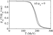
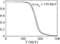
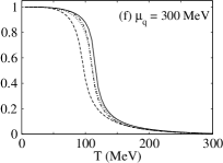
Figure 1: $\Phi$ (1a-1c) and the ratio $\rho_{sq}(T)/\rho_{sq}(vac)$ (1d-1f), of the different PNJL parametrizations, as a function of the temperature for some fixed values of $\mu_{q}$.

If we use only the PNJL model to construct the $T\times\mu_{q}$ diagram, the maxima of $(\partial\Phi/\partial T)$, and $(\partial\rho_{sq}/\partial T)$ at a given $\mu_{q}$ are used to define the transition temperature weise1 ; weise4 ; weise6 , in this case a crossover transition. Indeed, the strength of this mixing is utilized to find the value of $b$ in the FUKU08 potential fuku2 . Other similar criterium to find the transition point is to localize the maxima of the chiral, and Polyakov susceptibilities fuku1 ; weise6 . Here we will also use the Gibbs criterium to find such transition points since we are dealing with two different models to treat the different phases.

In Fig. 2 we show, at vanishing chemical potential, the behavior of some important thermodynamical quantities. The pressure, energy density and entropy density as a function of the temperature, and scaled by the respective Stefan-Boltzmann values $P_{SB}=\frac{37\pi^{2}T^{4}}{90}$, $\mathcal{E}_{SB}=3P_{SB}$, and $\mathcal{S}_{SB}=4P_{SB}/T$, are displayed in Figs. 2a-2c. In units of $T^{4}$, we furnish the called interaction measure given by $\mathcal{E}-3P$. This quantity show us how the model deviates from the noninteracting massless quark system, since in such regime its value is vanishing. Finally, as a function of the energy density, we see the evolution of the ratio $P/\mathcal{E}$ that is closely related with the sound velocity through $c_{s}^{2}=\frac{\partial P}{\partial\mathcal{E}}=\frac{\mathcal{E}\partial(P/\mathcal{E})}{\partial\mathcal{E}}+\frac{P}{\mathcal{E}}$. In the SB limit, one has ${c_{s}^{2}}_{SB}=P_{SB}/\mathcal{E}_{SB}=1/3$.

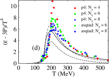
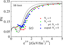
Figure 2: (Color online) (a-c): Pressure, energy density, and entropy density, in units of its respective SB values, versus $T$. (d): Interaction measure, in units of $T^{4}$, versus $T$. (e): Ratio $P/\mathcal{E}$ versus $\mathcal{E}^{1/4}$. All calculations at $\mu_{q}=0$. The three flavor lattice results were extracted from Refs. lat1 ; lat2 .

As a reference the recent QCD lattice results with temporal extent $N_{\tau}=4,6$ lat1 , and $N_{\tau}=8$ lat2 for the $2+1$ flavor system, in calculations with the improved fermion actions asqtad, and p4, are also shown in Fig. 2. Rigorous comparisons among lattice data and quantities such as the difference $\frac{P(T,\mu)}{T^{4}}-\frac{P(T,0)}{T^{4}}$ and the moments of the pressure, can be found, for example, in Refs weise1 ; weise2 ; ghosh , and weise2 ; weise4 ; weise5 ; weise6 , respectively.

Notice here the good agreement of the PNJL parametrizations and the lattice data, even the latter being originated from the 3 flavor system. We highlight RTW05 and RRW06 as being the models that better agree with the data. These results can be explained by the rescaling procedure adopted in the $T_{0}$ value (from $270$ MeV to $190$ MeV).

As mentioned in Ref. fuku2 , the FUKU08 model was not constructed to reproduce the Stefan-Boltzmann limit in high temperatures. This explains the deviation of the lattice data from temperatures higher than $200$ MeV even after our rescaling in the $b$ parameter of the model, from $b=0.03\Lambda^{3}$ to $b=0.007\Lambda^{3}$.

III Relativistic mean-field models

Different from the microscopic approach in which the nucleon-nucleon potentials are developed to reproduce the well established data of the few-nucleon physics, and where the basic informations about the many-body system are extracted, e.g., via Brueckner-Hartree-Fock methods, the Quantum Hadrodynamics (QHD), based on local Lagrangian densities, uses the nuclear matter bulk properties observables at zero temperature to adjust its free parameters and thereafter construct all the thermodynamics of the particular hadronic framework. One of the most used models coming from QHD is the nonlinear Walecka (or Boguta-Bodmer) boguta model, that is given by the following renormalizable Lagrangian density

$$\mathcal{L} = \bar{\psi}(i\gamma^{\mu}\partial_{\mu}-M)\psi+\frac{1}{2}\partial^{\mu}\sigma\partial_{\mu}\sigma-\frac{1}{2}m^{2}_{\sigma}\sigma^{2}-\frac{1}{4}F^{\mu\nu}F_{\mu\nu}+\frac{1}{2}m^{2}_{\omega}\omega_{\mu}\omega^{\mu}$$ (22)

$$- g_{\sigma}\sigma\bar{\psi}\psi-g_{\omega}\bar{\psi}\gamma^{\mu}\omega_{\mu}\psi-\frac{A}{3}\sigma^{3}-\frac{B}{4}\sigma^{4},$$

with $F_{\mu\nu}=\partial_{\nu}\omega_{\mu}-\partial_{\mu}\omega_{\nu}$, and the nucleon degree of freedom represented by the spinor $\psi$. The responsible mesons for the attractive, and repulsive parts of the nuclear interaction are described in this formulation by the scalar ($\sigma$), and vector ($\omega^{\mu}$) neutral fields, respectively. The saturation in nuclear matter is understood in the QHD by the almost vanishing value of $\,\Sigma=S+V\,$ at the saturation density, with $S$, and $V$ being the Lorentz meson potentials.. $M$, $m_{\sigma}$, and $m_{\omega}$ are, respectively, the masses of the nucleon, scalar, and vector mesons.

In their model, Boguta and Bodmer boguta considered the cubic and quartic self-interactions in the scalar field $\,\sigma\,$, in order to improve the original Walecka model walecka . In this version, the models are able to control through the fitting of their coupling constants, the values of the saturation density, binding energy ($B_{0}$) as well as the incompressibility ($K$), and the effective nucleon mass ($M^{*}$).

Through the Dirac equation of the model, one identifies its nucleon effective mass as

$$M^{*}=M+g_{\sigma}\sigma=M-G_{\sigma}^{2}[\rho_{s}+a(\Delta M)^{2}+b(\Delta M)^{3}],$$ (23)

with $G_{\sigma}^{2}=g_{\sigma}^{2}/m_{\sigma}^{2}$, $a=A/g_{\sigma}^{3}$, $b=B/g_{\sigma}^{4}$, and $\Delta M=M^{*}-M$. Let us remark here that this definition of effective mass, also called Dirac mass, is valid for the relativistic models. A deep discussion about other definitions and concepts of this physical quantity can be found in Ref. jaminon . The scalar and vector densities are written, at finite temperature, as

$$\rho_{s} = \left<\bar{\psi}\psi\right>=\frac{\gamma}{2\pi^{2}}\int_{0}^{\infty}\frac{M^{*}}{(k^{2}+{M^{*}}^{2})^{1/2}}k^{2}[f(k,T)+\bar{f}(k,T)]dk\quad\mbox{and}$$ (24)

$$\rho = \left<\bar{\psi}\gamma^{0}\psi\right>=\frac{\gamma}{2\pi^{2}}\int_{0}^{\infty}k^{2}[f(k,T)-\bar{f}(k,T)]dk,$$ (25)

with $\gamma=4$ for symmetric matter. The usual Fermi-Dirac distributions to particles and antiparticles are defined, respectively, by $f(k,T)=\left[e^{(\sqrt{k^{2}+{M^{*}}^{2}}-\nu)/T}+1\right]^{-1}$ and $\bar{f}(k,T)=\left[e^{(\sqrt{k^{2}+{M^{*}}^{2}}+\nu)/T}+1\right]^{-1}$, and the relation between the effective chemical potential, $\nu$, and the baryon chemical potential is given by $\mu_{B}=\nu+G_{\omega}^{2}\rho$.

From the energy-momentum tensor obtained through Eq. (22), one can obtain the pressure of the system, that reads

$$P_{\mbox{\tiny RMF}}=\frac{G_{\omega}^{2}\rho^{2}}{2}-\frac{(\Delta M)^{2}}{2G_{\sigma}^{2}}-\frac{a(\Delta M)^{3}}{3}-\frac{b(\Delta M)^{4}}{4}+\frac{\gamma}{6\pi^{2}}\int_{0}^{\infty}\frac{k^{4}}{(k^{2}+{M^{*}}^{2})^{1/2}}[f(k,T)+\bar{f}(k,T)]dk,$$ (26)

already written in terms of the mean-field approximation, as well as Eqs (23)-(25).

For the construction of the hadron-quark phase diagrams, we choose the following set of RMF parametrizations: Walecka (WAL) npb , NLB serot , NL2 reinhard , NLSH lalazissis , NLB1 reinhard , NL3 lalazissis , NLB2 reinhard , NLC serot , NL1 reinhard and NLZ2 bender . The WAL and NLZ2 models are chosen because their incompressibilities, $K=554.4$ MeV and $K=172.0$ MeV, respectively, indicate very hard and very soft EOS for infinite nuclear matter. The other models intermediate both. A full list of the nuclear matter saturation properties including $\rho_{0}$, $B_{0}$ and $m^{*}=M^{*}/M$ is found in Table 2 of Appendix B.

Important features can be highlighted concerning these relativistic models. At moderate temperatures, $T\lesssim 20$ MeV, a liquid-gas phase transition is predicted furn-serot . In Figs. 3a-3c we show the typical van der Waals behavior of the used parametrizations in the pressure versus density curves.

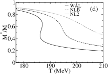
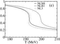
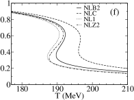
Figure 3: (Color online) (a)-(c) Pressure as a function of $\rho/\rho_{0}$ at $T=10$ MeV, and (d)-(f) Effective nucleon mass as a function of the temperature at $\mu_{B}=0$.

The Maxwell construction can be used to find the coexistence points, and consequently the coexistence curve. It was shown in Ref. jbatista that this curve, scaled by the critical parameters, is not universal in the liquid region due importance of the interactions in such phase. Another interesting feature of the RMF models occurs at high temperature regime ($T\sim 200$ MeV), where other kind of phase transition takes place. This scenario was studied by Theis et al theis in the context of the linear Walecka model at $\rho=\mu_{B}=0$. The authors have shown that the order of the phase transition depends on the values of the coupling constants used to fit $\rho_{0}$, and $B_{0}$. A signature of this transition is exhibited in the behavior of the nucleon effective mass as a function of the temperature, since an abrupt decreasing of $M^{*}$ characterizes a first order phase transition. In Figs. 3d-3f we present the high temperature regime of RMF models used in our work concerning the behavior of $M^{*}$ at zero baryon chemical potential. A recent study regarding the high temperature regime of RMF models at different number of nucleons and antinucleons ($\mu_{B}\neq 0$) was done in Ref. npb ; ratios .

IV RESULTS AND DISCUSSIONS

Now we present our mainly results regarding the hadron-quark phase diagrams, constructed from the Gibbs criteria shown in Eqs (1)-(2), defining first our notation for the transitions curves we will exhibit. We call the matching between the RMF models and the PNJL ones as the “RMF-PNJL” transition curves. When the transition is done with the MIT Bag model on the quark side, the modification is straightforward in the sense that the curve is denoted by “RMF-MIT”. Thus, the Gibbs criteria applied, for example, in the NL3 model together with the RRW06 one, generate the curve called NL3-RRW06. If the PNJL model is replaced by the MIT Bag one in this case, we denote this transition by NL3-MIT.

IV.1 RMF-PNJL transitions

Regarding the condition of equal pressures, we stress that the hadronic pressure, Eq. (26), was used to match the quark ones, Eq. (11), and Eq. (3) for the RMF-PNJL and RMF-MIT curves, respectively.

Let us remark here that for the RMF-PNJL transitions, we adopt the Gibbs criteria with the additional constraint that the RMF confined phase is actually matching the deconfined phase of the PNJL model. We only consider the solutions satisfying this condition. An example of this restriction is shown in Figs. 4a-4b for the NL3-RRW06, and NL3-FUKU08 matchings at $\mu_{B}=3\mu_{q}=660$ MeV.

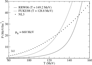
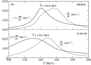
Figure 4: (a) Pressure as a function of the temperature for two of the PNJL models and the NL3 one. (b): $\partial\Phi/\partial T$ and $-\partial\xi/\partial T$ versus $T$, where $\xi=\rho_{sq}(T)/\rho_{sq}(vac)$. The transition temperature (see text) is given by $\overline{T}$. Both figures at $\mu_{B}=660$ MeV.

Notice that the FUKU08 and NL3 pressures cross each other at the temperature given by $T=128.8$ MeV, but since at this temperature the FUKU08 model is still in the confined phase (see the down panel of Fig. 4b), we did not consider this crossing for the NL3-FUKU08 phase diagram. Here we are following the same procedure used in Ref. weise1 concerning the definition of the transition temperature. In the case of the adopted rescaling for $T_{0}$ (in RTW05, RRW06 and DS10) and for $b$ (in FUKU08), the almost perfect coincidence between the peaks of the temperatures derivatives of $\Phi$ and $\rho_{sq}$ is lost. To circumvent this problem, for each chemical potential, the transition temperature $\overline{T}$, as the average of the different temperatures related to the peaks of $\partial\Phi/\partial T$ and $\partial\rho_{sq}/\partial T$. For the FUKU08 potential at $\mu_{B}=660$ MeV, this average is $\overline{T}=139.5$ MeV.

For the RRW06 and NL3 models, its pressures cross at $T=149.2$ MeV, where the RRW06 model already predicts the deconfinement, since its transition temperature is given by $\overline{T}=148.8$ MeV (see the up panel of Fig.. 4b). Therefore, the point in which $T=149.2$ MeV and $\mu_{B}=660$ MeV contributes to the NL3-RRW06 phase diagram.

In the next figure we present the hadron-quark phase diagrams for all the RMF-PNJL parametrizations used in this work.

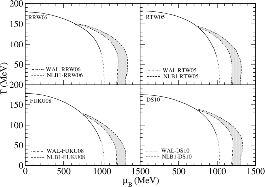
Figure 5: Hadron-quark phase diagrams in the $T\times\mu_{B}$ plane for the RMF-PNJL matching (grey band), and for the PNJL models themselves (full + dotted lines).

In Fig. 5, each individual panel depicts the diagrams where the matching between the models is done by keeping fixed the indicated quark model, and changing the hadronic one. In the same figure, for comparison, we also give the transition line of the phase diagram for each PNJL model itself constructed, as aforementioned, from the average of the temperatures related to the peaks of $\partial\Phi/\partial T$ and $\partial\rho_{sq}/\partial T$. The full (dotted) lines stand for the crossover (first order) transitions. It is important to stress here that there are different criteria to construct these PNJL transition curves, such as the choice between different peaks of $\partial\Phi/\partial T$ plsm and $\partial\rho_{sq}/\partial T$. This fact can favor the emergence of the quarkyonic phase, predicted in Ref. mclerran . A detailed study about these different choices and its consequences in the hadron-quark phase diagram is under progress.

An important feature regarding the PNJL curves are the values of the transition temperatures at vanishing chemical potential, $T_{c}(\mu=0)=179$ MeV, $181.8$ MeV, $177.3$ MeV, and $174.5$ MeV, respectively, for the RRW06, RTW05, FUKU08 and DS10 parametrizations. Notice that these values agree very well with the lattice QCD result for this quantity given by $T_{c}(\mu=0)\sim 170-190$ MeV star , or even with the more stringent value of $T_{c}(\mu=0)=173\pm 8$ MeV stringent . This nice agreement is completely destroyed if the original values of $T_{0}$ and $b$ are used in the construction of the PNJL curves. In this case, the values of $T_{c}(\mu=0)$ are higher than $200$ MeV for all the Polyakov potentials.

We also remark that the PNJL phase diagrams could also furnish other phases beside the confined/broken chiral symmetry, and deconfined/restored chiral symmetry ones, delimited by the full and dotted lines in Fig. 5. These specific phases are closely related to the instabilities of the ground state, present in any fermionic system at sufficiently low temperatures, that are overcame by the formation of the fermion pairs (in BCS theory, these are the so-called Cooper pairs). In particular, the quark system described by the PNJL models should also be affected in this regime, giving rise to the emergence of the two-flavor superconducting color (2SC), and the color flavor locked (CFL) phases. This phenomenology can be incorporated in the PNJL model, via inclusion of the diquark condensate term in its Lagrangian density. However, in this work we focus exclusively in the nonsuperconducting phases of the hadron-quark diagrams by treating only the simplest version of the PNJL model, in which the color condensates are not being taken into account. Very interesting studies concerning the consequences of the 2SC and CFL phases in the description of quark stars were performed for the NJL sc1 model, in which it is shown the role played by the diquark coupling strengths. Recently, this effect of the color superconductivity was also analyzed for the PNJL sc2 model, where a modified version of the DS10 Polyakov potential is used in the description of the quark core of massive hybrid stars.

Regarding the RMF-PNJL transitions themselves, we stress the following interesting results. First of all, notice that for all the RMF-PNJL matchings, one can delimit very narrow bands that encompass all the transition curves, being the WAL-PNJL and NLB1-PNJL matchings their extremes. This is not an obvious result since we are dealing with a large set of RMF models, in the sense that they present a range of very soft to very hard equations of state, i. e., from the NLZ2 model with $K=172$ MeV, up to the WAL one in which $K=554$ MeV. This result indicates that at least for RMF models with scalar self-interactions of third and fourth order, all of them will predict very similar behavior concerning the hadron-quark phase transition, in connection with PNJL models.

Our systematic study still shows that the additional constraint exemplified in Figs. 4a and 4b, are useful to define the CEP’s of the RMF-PNJL transitions, given approximately by ($\mu_{B}^{\mbox{\tiny CEP}}=650$ MeV, $T^{\mbox{\tiny CEP}}=149$ MeV), ($750$ MeV, $142$ MeV), ($750$ MeV, $126$ MeV), and ($750$ MeV, $138$ MeV), respectively, for the RMF-RRW06, RMF-RTW05, RMF-FUKU08, and RMF-DS10 transitions. In a different way, the CEP is also defined in Ref. gyshao . Notice how this restriction avoids the hadron-quark phase transition curves go inside the confined phases predicted by the PNJL transitions.

This situation is completely modified if we use the original values of $T_{0}$ and $b$ of the PNJL models. In this case there is no CEP for the RMF-PNJL transitions, in the sense that there is no transition inside the hadron phase of the PNJL models themselves. The only exception is for the RMF-FUKU08 transitions, that present the same qualitative behavior shown in Fig. 5 for the calculations done with the original value $b=0.03\Lambda^{3}$.

We still highlight here a very important physical consequence of the construction of the hadron-quark phase transitions via connection of the RMF and PNJL models. The panels in Fig. 5 clearly show us that the hadronic degrees of freedom present in the RMF models, make the system much more resistant to the quark liberation, in function of the density/chemical potential increasing, when compared with a system only described by the PNJL model. The physical origin of this important difference is due to the very known repulsive nature of the nuclear force, represented in the RMF models by the vector interaction, which strength is controlled by the coupling constant $g_{\omega}$, see Eq. (22) (in nuclear matter equations of state, this strength is actually controlled by the ratio $G_{\omega}=g_{\omega}/m_{\omega}$). The repulsion makes the system support more strongly isothermal compressions. In other words, the RMF-PNJL transitions predict confined (hadron) phases larger than those obtained exclusively with the PNJL models. This region of highly compressed matter of the hadron-quark phase diagram, is expected to be reached in the new experiments, such as the planned to occur in the new facilities FAIR/GSI fair , and NICA/JINR nica . Therefore, it will be explicit what is the magnitude of the role played by the repulsive interaction part of the nuclear force, even guiding possible selections of better parametrizations.

The difference between the RMF-PNJL and the PNJL transitions can be decreased if we use PNJL models that also contain repulsive interactions, i.e., that present vector fields in its structure. Notice that the PNJL models used here are based on a structure that present only attractive interactions. There is no explicit terms proportional to the quark density in Eq. (6), coming from vector-type fields. Moreover, as pointed out in Ref. fuku2 , there is no constraint at all for the choice of the strength of this kind of interaction in the PNJL model. A study about the determination of this magnitude, by making minimum the difference shown in Fig. 5, is underway.

IV.2 Comparison with RMF-MIT transitions

We perform now, systematic comparisons between the RMF-PNJL transitions with RMF-MIT ones, in order to verify explicitly the role played by the dynamical confinement of the PNJL models in the hadron-quark phase diagrams. To construct such curves, we use the particular value of $B^{1/4}=238$ MeV, that furnish a critical temperature at vanishing chemical potential consistent with the lattice simulation results.

Firstly, we show in Fig. 6 the behavior of RMF-MIT curves in the $T\times\mu_{B}$ plane for all the hadronic parametrizations.

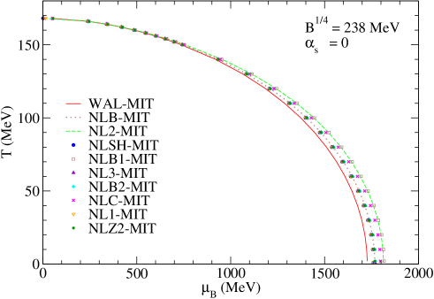
Figure 6: (Color online) Phase diagrams in the $T\times\mu_{B}$ plane for the RMF-MIT matching. In the Eq. (3), we have used $B^{1/4}=238$ MeV and $\alpha_{s}=0$.

Some interesting points about these particular transitions have to be mentioned here. Notice that differently from the RMF-PNJL diagrams, all the RMF-MIT curves start at the same temperature, $T_{c}(\mu=0)=168$ MeV. There is no critical end points as shown in Fig. 5. Similar behavior between the curves can be seen at $T=0$, since all used models are lied in a narrow band in this region. They lie in the range around $1190$ MeV $<\mu_{B}<1310$ MeV ($1730$ MeV $<\mu_{B}<1810$ MeV) for the RMF-PNJL (RMF-MIT) curves. For the RMF-MIT transitions, this behavior is strongly changed if the RMF models with higher order terms in the vector field, or even mixing terms between $\sigma$ and $\omega_{\mu}$ are used on the hadronic side. This is the case, for example, for the models used in Ref. jphysg . We stress that the behavior shown in Figs. 5 and 6 is characteristic of the transitions in which the used RMF parametrizations only contain cubic and quartic self-coupling terms in the scalar field $\sigma$, see Eq. (22).

This almost model independent result for the hadron-quark transition at $T=0$ for the RMF-PNJL/MIT matchings, see Figs. 5 and 6, is not surprising from the point of view of the PNJL models, since the Polyakov potentials related to the RRW06, RTW05, and FUKU08 models vanish in the zero temperature regime, see Eqs. (15)-(17), and the modified Fermi-Dirac distributions, Eqs. (9) and (10), behave as the conventional ones in the $T\rightarrow 0$ limit. In particular, the DS10 Polyakov potential vanish at $T=0$ also due to $\Phi=0$, see Eq.. (18). That is, all the PNJL models used here are converted in the same model at $T\rightarrow 0$, in this case, the NJL one on the quark side. This is also the case in the RMF-MIT transitions, i.e., one has only one parametrization of the quark model since we fixed $B$ and $\alpha_{s}$ in Eq. (3) to construct the diagrams shown in Fig. 6. We remark that by construction, at $T=0$ all the RMF models lead to different bulk nuclear matter properties. We stress here that this almost model independence in the $\mu_{B}$ value at $T=0$ can be relevant to the study of hybrid stars, composed by a quark core and a hadron crust malheiro1 ; malheiro2 .

In order to see the effect of the dynamical confinement present in the PNJL models in the RMF-PNJL transition curves, we explicitly compare the phase diagrams of both, RMF-PNJL/RMF-MIT phase diagrams in the same Fig. 7.

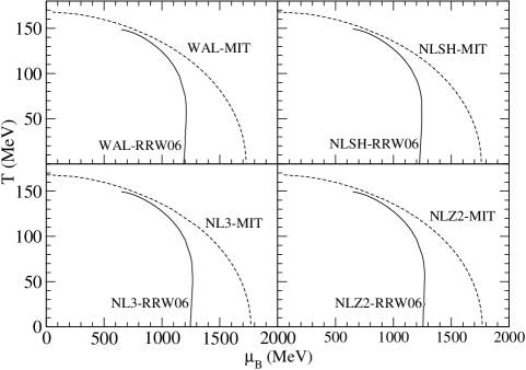
Figure 7: RMF-PNJL/RMF-MIT phase diagrams in the $T\times\mu_{B}$ plane for some hadronic parametrizations. Here we also use $\alpha_{s}=0$.

In this figure one can clearly see that the hadronic region predicted for the RMF-PNJL matchings is always smaller than that obtained from the RMF-MIT ones, i.e., the quark degrees of freedom emerge before in the RMF-PNJL curves. Although we have presented only the transition curves shown in Fig. 7, we streamline that all the other diagrams follow the same pattern, thus the respective RMF-PNJL/RMF-MIT curves can be considered as representatives of all the models treated in this work. An enlarged view of these features can be viewed in Fig. 8.

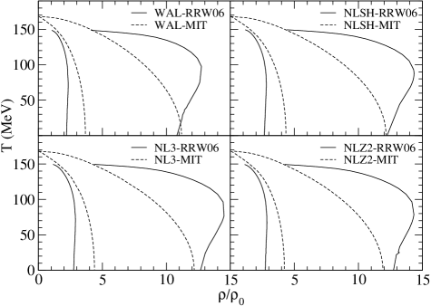
Figure 8: RMF-PNJL/RMF-MIT phase diagrams in the $T\times\rho$ plane.

In this figure, despite present the larger hadron regions, that are delimited by the left branches of the curves, the RMF-MIT diagrams show that the mixed phase containing both hadrons and quarks is actually smaller in such diagrams. This difference, specifically at $T=0$ is extremely important to the study of hybrid stars, since its quark core is directly affected by the maximum density of the mixed phase malheiro1 ; malheiro2 .

As our final remark, we point out that in the construction of the RMF-PNJL diagrams, we proceed in a different way that used in Ref. ciminale . In this reference, the authors used a bag constant also in the PNJL pressure in order to ensure that the quark pressure is less than the hadronic one in the confined phase. Here we force $P_{\mbox{\tiny PNJL}}(T=\rho_{q}=0)=0$, by subtracting from the grand-potential its vacuum value.

V SUMMARY AND CONCLUSIONS

In this work we have studied the hadron-quark phase diagrams using two different models in the description of the distinct phases. The quark degrees of freedom were described via the recently suggested PNJL model fuku1 which incorporates the confinement phenomenon in the previous NJL one. As one of our results, we compared the current PNJL parametrizations that differ each other by the Polyakov potential $\mathcal{U}(\Phi,\Phi^{*},T)$. We used the polynomial form RTW05 weise1 , the logarithmic RRW06 weise2 ; weise3 ; weise4 ; weise5 ; weise6 ; weise7 ; ratti ; costa , the FUKU08 fuku2 , and also included the DS10 schramm one that presents a chemical potential dependence. The Fig. 2 show the good agreement with the lattice data, specially for the RRW06 and RTW05 parametrizations even the PNJL models being treated in the two-flavor system. It was also shown that the parametrizations furnish similar results for the analyzed thermodynamical quantities. The good agreement with the lattice data remains valid even for the transition temperature at vanishing chemical potential, predicted to be given by $T_{c}(\mu=0)=173\pm 8$ MeV stringent . Our calculations give the values of $T_{c}(\mu=0)=179$ MeV, $181.8$ MeV, $177.3$ MeV, and $174.5$ MeV, respectively, for the RRW06, RTW05, FUKU08 and DS10 PNJL models used in this work. We still remark that these nice values are obtained with the rescaling of the parameters $T_{0}$ (RRW06, RTW05 and DS10) and $b$ (FUKU08).

On the hadronic side, we have used the well known RMF nonlinear Walecka models in its version that contains cubic and quartic self-coupling in the scalar field. We chose to deal with a set of these models that encompasses several incompressibilities values, representing very hard and soft equations of state.

Regarding the phase diagrams, we have constructed the RMF-PNJL curves using the Gibbs criteria and the additional constraint that the RMF pressure matches the PNJL one only in its deconfined phase. This condition is exemplified in Figs. 4a-4b, and played an important role in the final diagrams, since it determines the critical end points given approximately by ($\mu_{B}^{\mbox{\tiny CEP}}=650$ MeV, $T^{\mbox{\tiny CEP}}=149$ MeV), ($750$ MeV, $142$ MeV), ($750$ MeV, $126$ MeV), and ($750$ MeV, $138$ MeV), respectively, for the RMF-RRW06, RMF-RTW05, RMF-FUKU08, and RMF-DS10 transitions. Moreover, it is also important to stress that all these transitions furnish very similar results in a such way that one can define a very narrow band in the $T\times\mu$ plane encompassing all the RMF-PNJL curves, being the WAL-PNJL and NLB1-PNJL the limiting curves of these bands, see Fig. 5. This is a surprising result since we are dealing with a very large class of RMF models. In principle, there is no reason to the hadron-quark phase diagram behaves in a very similar way with such variety of RMF parametrizations.

Other important result concerning the RMF-PNJL phase diagrams is their different predictions compared to those obtained exclusively with the PNJL quark models. We found that the hadron phase described by the RMF-PNJL transitions is meaningfully larger than that predicted by the PNJL ones, i.e., the RMF-PNJL hadron phase is more resistant to the isothermal compressions. Physically, such difference is due to the repulsive part of the nuclear force described in the RMF models by the vector field interaction. Therefore, one become clear that there are very different results in treating the hadron-quark phase transition via two distinct models, taking into account the different degrees of freedoms (hadrons and quarks), or only via quark models, even being the latter very realistic ones as the PNJL models that nicely agree with lattice QCD data, and where the dynamical confinement is considered in the NJL model through the Polyakov loop. We also remark that the region where the different descriptions do not agree each other will can be accessed in the future experiments planned to occur in the new facilities FAIR/GSI fair , and NICA/JINR nica .

As a final result, we compared the RMF-PNJL curves with that constructed by the matching between the hadronic models and the MIT Bag one, that incorporates the confinement via inclusion of the bag constant $B$. The Figs. 7 and 8 show that the dynamical confinement predicted in the PNJL model force the hadronic phase of the RMF-PNJL diagrams be smaller than the RMF-MIT ones. Curiously, the opposite occurs for the mixed phase, where hadrons and quarks coexist, see Fig. 8. These comparisons were done by assuming the value of $B^{1/4}=238$ MeV for the MIT bag model, that nicely predicts a value of $168$ MeV for the transition temperature at vanishing chemical potential, see Fig. 6.

Appendix A Zero temperature expressions for the PNJL model: NJL sector

In this appendix we show the zero temperature expressions of the PNJL model, that actually are exactly the NJL ones, and give the remaining parameters needed to define the PNJL models presented in our work. We refer here only to that parametrizations that do not present contributions containing the traced Polyakov loop in the $T=0$ regime, i.e., we only consider the cases in which $\mathcal{U}(\Phi,\Phi^{*},T=0)=0$.

In the $T=0$ regime, the energy density given in Eq. (13), and the scalar density in Eq. (8), are replaced by

$$\mathcal{E}_{\mbox{\tiny PNJL}}(T=0) = \frac{G{\rho_{sq}}^{2}}{2}+\frac{\gamma_{q}}{8\pi^{2}}\left[k_{Fq}^{4}\,\xi\left(\frac{M_{q}}{k_{Fq}}\right)-\Lambda^{4}\,\xi\left(\frac{M_{q}}{\Lambda}\right)\right],\qquad\mbox{and}$$ (27)

$$\rho_{sq}(T=0) = \frac{\gamma_{q}M_{q}}{4\pi^{2}}\left[k_{Fq}^{2}\zeta\left(\frac{M_{q}}{k_{Fq}}\right)-\Lambda^{2}\zeta\left(\frac{M_{q}}{\Lambda}\right)\right]$$ (28)

with

$$\xi(z) = \left(1+\frac{z^{2}}{2}\right)\sqrt{1+z^{2}}-\frac{z^{4}}{2}\mbox{ln}\left(\frac{\sqrt{1+z^{2}}+1}{z}\right),\qquad\mbox{and}$$ (29)

$$\zeta(z) = \sqrt{1+z^{2}}-\frac{z^{2}}{2}\mbox{ln}\left(\frac{\sqrt{1+z^{2}}+1}{\sqrt{1+z^{2}}-1}\right),$$ (30)

where $k_{Fq}$ is the Fermi momentum of the quark. The quark density is $\rho_{q}=\frac{\gamma_{q}}{6\pi^{2}}k_{Fq}^{3}$, and the pressure reads

$$P_{\mbox{\tiny PNJL}}(T=0)=\mu_{q}\rho_{q}-\mathcal{E}_{\mbox{\tiny PNJL}}(T=0),$$ (31)

with the quark chemical potential given by $\mu_{q}=(k_{Fq}^{2}+M_{q}^{2})^{1/2}$.

Thus, the respective vacuum expressions obtained at $k_{Fq}=0$ are

$$\mathcal{E}_{\mbox{\tiny vac}} = \frac{G{\rho_{sq}^{\mbox{\tiny vac}}\,}^{2}}{2}-\frac{\gamma_{q}\Lambda^{4}}{8\pi^{2}}\,\xi\left(\frac{M_{q}^{\mbox{\tiny vac}}}{\Lambda}\right),\qquad\mbox{and}$$ (32)

$$\rho_{sq}^{\mbox{\tiny vac}} = -\frac{\gamma_{q}M_{q}^{\mbox{\tiny vac}}\Lambda^{2}}{4\pi^{2}}\zeta\left(\frac{M_{q}^{\mbox{\tiny vac}}}{\Lambda}\right).$$ (33)

So, fixing the values $m_{\pi}=140.51$ MeV, $f_{\pi}=94.04$ MeV, and $|\left<\bar{u}u\right>|^{1/3}=251.32$ MeV, and using Eq. (33) together with the Gell-Mann-Oakes-Renner relation $m_{\pi}^{2}f_{\pi}^{2}=-M_{0}\rho_{sq}$, and

$$f_{\pi}^{2}=\frac{N_{s}N_{c}M_{q}^{2}}{2\pi^{2}N_{f}}\int_{0}^{\Lambda}\frac{k^{2}dk}{(k^{2}+M_{q}^{2})^{3/2}},$$ (34)

one obtains $\Lambda=651$ MeV, $M_{0}=5.5$ MeV, and $G=10.08$ GeV^-2. The constituent vacuum quark mass obtained from these values is $M_{q}^{\mbox{\tiny vac}}=325.53$ MeV.

The assumption $\mathcal{E}_{\mbox{\tiny PNJL}}(T=\rho_{q}=0)=0$ leads to the following final expression for the energy density,

$$\mathcal{E}_{\mbox{\tiny PNJL}}(T=0) = \frac{G{\rho_{sq}}^{2}}{2}+\frac{\gamma_{q}}{8\pi^{2}}\left[k_{Fq}^{4}\,\xi\left(\frac{M_{q}}{k_{Fq}}\right)-\Lambda^{4}\,\xi\left(\frac{M_{q}}{\Lambda}\right)\right]-\Omega_{\mbox{\tiny vac}},$$ (35)

where $\Omega_{\mbox{\tiny vac}}\equiv\mathcal{E}_{\mbox{\tiny vac}}$. Notice that the same condition also ensures that $P_{\mbox{\tiny PNJL}}(T=\rho_{q}=0)=0$. For the parameters aforementioned one has that $|\Omega_{\mbox{\tiny vac}}|^{1/4}=409.15$ MeV. In this work we have considered this value of $\Omega_{\mbox{\tiny vac}}$ in the Polyakov potentials, even for the DS10 parametrization.

Appendix B Parametrizations of the RMF models

Some important saturation quantities of the RMF models used in our work are listed in the next table.

Table 2: Saturation properties of the RMF models.

Model	$\rho_{0}$ (fm-3)	$B_{0}$ (MeV)	$m^{*}$	$K$ (MeV)
Walecka (WAL)	$0.150$	$-15.75$	$0.54$	$554.38$
NLB	$0.148$	$-15.75$	$0.61$	$420.00$
NL2	$0.146$	$-17.03$	$0.67$	$399.20$
NLSH	$0.146$	$-16.35$	$0.60$	$355.36$
NLB1	$0.162$	$-15.74$	$0.62$	$280.00$
NL3	$0.148$	$-16.30$	$0.60$	$271.76$
NLB2	$0.162$	$-15.73$	$0.56$	$245.10$
NLC	$0.148$	$-15.75$	$0.63$	$225.00$
NL1	$0.152$	$-16.42$	$0.57$	$211.70$
NLZ2	$0.151$	$-16.07$	$0.58$	$172.00$

The binding energy is calculated from the energy density at $T=0$,

$$\mathcal{E}_{\mbox{\tiny RMF}}=\frac{G_{\omega}^{2}\rho^{2}}{2}+\frac{(\Delta M)^{2}}{2G_{\sigma}^{2}}+\frac{a(\Delta M)^{3}}{3}+\frac{b(\Delta M)^{4}}{4}+\frac{\gamma}{2\pi^{2}}\int_{0}^{k_{F}}(k^{2}+{M^{*}}^{2})^{1/2}dk,$$ (36)

by $B_{0}=\mathcal{E}_{\mbox{\tiny RMF}}/\rho-M$ at $\rho=\rho_{0}$. The incompressibility, $K=9\frac{\partial P}{\partial\rho}$, reads

$$K_{\mbox{\tiny RMF}} = 9G_{\omega}^{2}\rho+\frac{3k_{F}^{2}}{E^{*}_{F}}-\frac{9{M^{*}}^{2}\rho}{{E^{*}_{F}}^{2}\left[\frac{1}{G_{\sigma}^{2}}+2a\Delta M+3b(\Delta M)^{2}+3\left(\frac{\rho_{s}}{M^{*}}-\frac{\rho}{E^{*}_{F}}\right)\right]},$$ (37)

with $E_{F}^{*}=(k_{F}^{2}+{M^{*}}^{2})^{1/2}$.

References

- (1) C. Höhne, K. E. Choi, V. Dobyrn, et. al., Nucl. Instr.. and Meth. A 639, 294 (2011); P. Senger, T. Galatyuk, et. al., J.Phys. G: Nucl. Part. Phys. 36, 064037 (2009); S. Chattopadhyay, J. Phys. G: Nucl. Part. Phys. 35, 104027 (2008); J. M. Heuser (CBM Collaboration), Nucl. Phys. A830, 563c (2009); http://www.gsi.de/fair.
- (2) A. N. Sissakian, A. S. Sorin, and V. D. Toneev, arXiv:nucl-th/0608032; http://nica.jinr.ru/.
- (3) J. B. Kogut, Rev. Mod. Phys. 51, 659 (1979); Rev. Mod. Phys. 55, 775 (1983); H. J. Rothe, Lattice gauge theories. An introduction (World Scientific, Singapore, 1997).
- (4) D. P. Landau and K. Binder, A guide to Monte Carlo simulations in Statistical Physics (Cambridge University Press, Cambridge, 2000).
- (5) K. Splittorff, and J. J. M. Verbaarschot, Phys. Rev. Lett. 98, 031601 (2007).
- (6) C. R. Allton et al., Phys. Rev. D 66, 074507 (2002); C. R. Allton et al., Phys. Rev. D 68, 014507 (2003); C. R. Allton et al., Phys. Rev. D 71, 054508 (2005).
- (7) Z. Fodor and S.D. Katz, Phys. Lett. B 534 87 (2002); J. High Energy Phys. 03, 014 (2002); Z. Fodor, S. D. Katz, and K. K. Szabo, Phys. Lett. B 568, 73 (2003).
- (8) E. Laermann, O. Philipsen, Annu. Rev. Nucl. Part. Sci. 53, 163 (2003).
- (9) P. de Forcrand and O. Philipsen, Nucl. Phys. B642, 290 (2002); Nucl. Phys. B673, 170 (2003); M. D’Elia and M. P. Lombardo, Phys. Rev. D 67, 014505 (2003); 70, 074509 (2004); M. D’Elia, F. Di Renzo, and M. P. Lombardo, Phys. Rev. D 76, 114509 (2007).
- (10) Z. Fodor, S. D. Katz, and C. Schmidt, J. High Energy Phys. 03, 121 (2007).
- (11) D. J. Gross, and F. Wilczek, Phys. Rev. Lett. 30, 1343 (1973); H. D. Politzer, Phys. Rev. Lett. 30, 1346 (1973).
- (12) A. Chodos, R. L. Jaffe, K. Johnson, C. B. Thorn and V. F. Weisskopf, Phys. Rev. D 9, 3471 (1974); A. Chodos, R. L. Jaffe, K. Johnson, C. B. Thorn, Phys. Rev. D 10, 2599 (1974); T. DeGrand, R. L. Jaffe, K. Johnson, J. Kiskis, Phys. Rev. D 12, 2060 (1975).
- (13) Y. Nambu, G. Jona-Lasinio, Phys. Rev. 122, 345 (1961); 124, 246 (1961).
- (14) M. Buballa, Phys. Rep. 407, 205 (2005).
- (15) U. Vogl and W. Weise, Prog. Part. Nucl. Phys. 27, 195 (1991); S. P. Klevansky, Rev. Mod. Phys. 64, 649 (1992); T. Hatsuda and T. Kunihiro, Phys. Rep. 247, 221 (1994).
- (16) M. Hanauske, L. M. Satarov, I. N. Mishustin, H. Stöcker, and W. Greiner, Phys. Rev. D 64, 043005 (2001).
- (17) M. Alford, M. Braby, M. Paris, and S. Reddy, Astrophys. J. 629, 969 (2005).
- (18) P. Wang, A. W. Thomas, and A. G. Williams, Phys. Rev. C 75, 045202 (2007).
- (19) E. S. Bowman, and J. I. Kapusta, Phys. Rev. C 79, 015202 (2009).
- (20) P. Ring and P. Schuck, The Nuclear Many-Body Problem (Springer, Heidelberg, 1980).
- (21) G. Y. Shao, M. Di Toro, V. Greco, M. Colonna, S. Plumari, B. Liu, and Y. X. Liu, Phys. Rev. D 84, 034028 (2011).
- (22) A. Delfino, M. Chiapparini, M. E. Bracco, L. Castro, and S. E. Epsztein, J. Phys. G 27, 2251 (2001); A. Delfino, J. B. Silva, M. Malheiro, M. Chiapparini, and M. E. Bracco, J. Phys. G 28, 2249 (2002).
- (23) R. Cavagnoli, C. Providência, and D. P. Menezes, Phys. Rev. C 83, 045201 (2011).
- (24) U. Heinz, P. R. Subramanian, H. Stöcker and W. Greiner, J. Phys. G 12, 1237 (1986).
- (25) Bo-Qiang Ma, Qi-Ren Zhang, D. H. Rischke and W. Greiner, Phys. Lett. B 315, 29 (1993).
- (26) K. Fukushima, Phys. Lett. B 591, 277 (2004).
- (27) C. Ratti, M. A. Thaler, and W. Weise, Phys. Rev. D 73, 014019 (2006).
- (28) C. Ratti, S. Roessner, M.A. Thaler, and W. Weise, Eur. Phys. J. C 49, 213 (2007).
- (29) C. Ratti, S. Roessner, and W. Weise, Phys. Lett. B 649, 57 (2007).
- (30) S. Rossner, C. Ratti, and W. Weise, Phys. Rev. D 75, 034007 (2007).
- (31) C. Ratti, S. Roessner, and W. Weise, J. Phys. G 34, S647 (2007).
- (32) S. Roessner, T. Hell, C. Ratti, and W. Weise, Nucl. Phys. A814, 118 (2008).
- (33) T. Hell, S. Rossner, M. Cristoforetti, and W. Weise, Phys. Rev. D 79, 014022 (2009).
- (34) H. Hansen, W. M. Alberico, A. Beraudo, A. Molinari, M. Nardi, and C. Ratti, Phys. Rev. D 75, 065004 (2007).
- (35) P. Costa, M. C. Ruivo, C. A. de Sousa, H. Hansen, and W. M. Alberico, Phys. Rev. D 79, 116003 (2009).
- (36) K. Fukushima, Phys. Rev. D 77, 114028 (2008).
- (37) V. A. Dexheimer, and S. Schramm, Phys. Rev. C 81, 045201 (2010); V. A. Dexheimer, and S. Schramm, Nucl. Phys. A827, 579 (2009).
- (38) M. Cheng, N. H. Christ, S. Datta, et. al., Phys. Rev. D 77, 014511 (2008).
- (39) A. Bazavov, T. Bhattacharya, M. Cheng, et. al., Phys. Rev. D 80, 014504 (2009).
- (40) S. K. Ghosh, T. K. Mukherjee, M. G. Mustafa, and R. Ray, Phys. Rev. D 73, 114007 (2006).
- (41) J. Boguta, and A. R. Bodmer, Nucl. Phys. A292, 413 (1977).
- (42) B. D. Serot, and J. D. Walecka, Advances in Nuclear Physics (Plenum, New York, 1986), Vol. 16.
- (43) M. Jaminon and C. Mahaux, Phys. Rev. C 40, 354 (1989); Nucl. Phys. A365, 371 (1981).
- (44) O. Lourenço, M. Dutra, V. S. Timóteo, and A. Delfino, Nucl. Phys. B, Proc. Suppl. 199, 349 (2010).
- (45) B. D. Serot, and J. D. Walecka, Int. Jour. Mod. Phys. E 6, 515 (1997).
- (46) P. -G. Reinhard, Rep. Prog. Phys. 52, 439 (1989).
- (47) G. A. Lalazissis, J. Konig, and P. Ring, Phys. Rev. C 55, 540 (1997).
- (48) M. Bender, K. Rutz, P. -G. Reinhard, J. A. Maruhn, and W. Greiner, Phys. Rev. C 60, 034304 (1999).
- (49) R. J. Furnstahl and B. D. Serot, Phys. Rev. C 41, 262 (1990).
- (50) J. B. Silva, O. Lourenço, A. Delfino, J. S. Sá Martins, and M. Dutra, Phys. Lett. B 664, 246 (2008).
- (51) J. Theis et al., Phys. Rev. D 28, 2286 (1983).
- (52) A. Delfino, M. Jansen, and V. S. Timóteo, Phys. Rev. C 78, 034909 (2008).
- (53) H. Mao, J. Jin, and M. Huang, J. Phys. G 37, 035001 (2010).
- (54) L. McLerran, and R.D. Pisarski, Nucl. Phys. A796, 83 (2007); L. Mclerran, Nucl. Phys. A830, 709c (2009); L. McLerran, K. Redlich, and C. Sasaki, Nucl. Phys. A824, 86 (2009).
- (55) M. M. Aggarwal, et. al., (STAR Collaboration), Phys. Rev. Lett. 105, 022302 (2010).
- (56) F. Karsch, E. Laermann, and A. Peikert, Nucl. Phys. B605, 579 (2001); F. Karsch, Nucl. Phys. A698, 199 (2002); F. Karsch, Lect. Notes Phys. 583, 209 (2002); O. Kaczmarek and F. Zantow, Phys. Rev. D 71, 114510 (2005);
- (57) D. Blaschke, S. Fredriksson, H. Grigorian, A. M. Oztas, and F. Sandin, Phys. Rev. D 72, 065020 (2005).
- (58) D. Blaschke, J. Berdermann, and R. Lastowiecki, Prog. Theor. Phys. Suppl. 186, 81 (2010).
- (59) J. C. Coelho, C. H. Lenzi, M. Malheiro, R. M. Marinho, and M. Fiolhais, Int. Jour. Mod. Phys. D 19, 1521 (2010).
- (60) M. Malheiro, M. Fiolhais, and A. R. Taurines, J. Phys. G 29, 1045 (2003).
- (61) M. Ciminale, R. Gatto, N.D. Ippolito, G. Nardulli, M. Ruggieri, Phys. Rev. D 77, 054023 (2008).