Constraining Bilinear $R$-Parity Violation from Neutrino Masses

Abstract

We confront the $R$-parity violating MSSM model with the neutrino oscillation data. Investigating the 1–loop particle–sparticle diagrams with additional bilinear insertions on the external neutrino lines we construct the relevant contributions to the neutrino mass matrix. A comparison of the so-obtained matrices with the experimental ones assuming normal or inverted hierarchy and taking into account possible CP violating phases, allows to set constraints on the values of the bilinear coupling constants. A similar calculation is presented with the input from the Heidelberg–Moscow neutrinoless double beta decay experiment. We base our analysis on the renormalization group evolution of the MSSM parameters which are unified at the GUT scale. Using the obtained bounds we calculate the contributions to the Majorana neutrino transition magnetic moments.

I Supersymmetric model with $R$-parity violation

The recent confirmation of neutrino oscillations nu-osc gives a clear signal of existence of physics beyond the standard model of particles and interactions (SM). Among many exotic proposals the introduction of supersymmetry (SUSY) proved to be both elegant and effective in solving some of the drawbacks of the SM. The minimal supersymmetric standard model (MSSM) (a comprehensive review can be found in mssm ) populates the so-called desert between the electroweak and the Planck scale with new heavy SUSY particles, thus removing the scale problem. What is more, using the MSSM renormalization group equations for gauge couplings indicates that there is a unification of $g_{1}$, $g_{2}$ and $g_{3}$ around $m_{GUT}\approx 1.2\times 10^{16}\hbox{ GeV}$ which means that MSSM in a somehow natural way includes Grand Unified Theories (GUTs). This model is also characterized by a heavier Higgs boson, comparing with the Higgs boson predicted by SM, which is in better agreement with the known experimental data. New interactions present in MSSM lead to many exotic processes which opens a completely new field of research.

Building the minimal supersymmetric version of the Standard Model one usually assumes the conservation of the $R$-parity, defined as $R=(-1)^{3B+L+2S}$, where $B$ is the baryon number, $L$ the lepton number, and $S$ the spin of the particle. The definition implies that all ordinary SM particles have $R=+1$ and all their superpartners have $R=-1$. In theories preserving $R$-parity the product of $R$ of all the interacting particles in a vertex of a Feynman diagram must be equal to $1$. This implies that the lepton and baryon numbers are conserved, and that SUSY particles are not allowed to decay to non-SUSY ones. It follows that the lightest SUSY particle (usually the lightest neutralino $\tilde{\chi}^{0}_{1}$) must remain stable, giving a good natural candidate for cold dark matter. All this makes the $R$-parity conserving models very popular.

In practice, however, the $R$-parity conservation is achieved by neglecting certain theoretically allowed terms in the superpotential. Casting such hand-waving approach away, one should retain these terms, finishing with an $R$-parity violating (RpV) model, with richer phenomenology and many even more exotic interactions aul83 ; valle ; np ; rbreaking . The RpV models provide mechanisms of generating Majorana neutrino masses and magnetic moments, describe neutrino decays, SUSY particles decays, exotic nuclear processes like the neutrinoless double beta decay, and many more. Being theoretically allowed, RpV SUSY theories are interesting tools for studying the physics beyond the Standard Model. The many never-observed processes allow also to find severe constraints on the non-standard parameters of these models, giving an insight into physics beyond the SM.

The violation of the $R$-parity may be introduced in a few different ways. In the first one $R$-parity violation is introduced as a spontaneous process triggered by a non-zero vacuum expectation value of some scalar field aul83 . Another possibilities include the introduction of additional bi- valle or trilinear rbreaking RpV terms in the superpotential, or both. In the following we incorporate the explicit RpV breaking scenario.

The $R$-parity conserving part of the superpotential of MSSM is usually written as

$$W^{MSSM} = \epsilon_{ab}[(\mathbf{Y}_{E})_{ij}L_{i}^{a}H_{u}^{b}\bar{E}_{j}+(\mathbf{Y}_{D})_{ij}Q_{ix}^{a}H_{d}^{b}\bar{D}_{j}^{x}$$ (1)

$$+ (\mathbf{Y}_{U})_{ij}Q_{ix}^{a}H_{u}^{b}\bar{U}_{j}^{x}+\mu H_{d}^{a}H_{u}^{b}],$$

while its RpV part reads

$$W^{RpV} = \epsilon_{ab}\left[\frac{1}{2}\lambda_{ijk}L_{i}^{a}L_{j}^{b}\bar{E}_{k}+\lambda^{\prime}_{ijk}L_{i}^{a}Q_{jx}^{b}\bar{D}_{k}^{x}\right]$$ (2)

$$+ \frac{1}{2}\epsilon_{xyz}\lambda^{\prime\prime}_{ijk}\bar{U}_{i}^{x}\bar{D}_{j}^{y}\bar{D}_{k}^{z}+\epsilon_{ab}\kappa^{i}L_{i}^{a}H_{u}^{b}.$$

The Y’s are 3$\times$3 Yukawa matrices. $L$ and $Q$ are the $SU(2)$ left-handed doublets while $\bar{E}$, $\bar{U}$ and $\bar{D}$ denote the right-handed lepton, up-quark and down-quark $SU(2)$ singlets, respectively. $H_{d}$ and $H_{u}$ mean two Higgs doublets. We have introduced color indices $x,y,z=1,2,3$, generation indices $i,j,k=1,2,3=e,\mu,\tau$ and the SU(2) spinor indices $a,b=1,2$.

As far as the (in principle unknown) RpV coupling constants are concerned, the most popular approach is to neglect the bilinear terms and to discuss the effects connected with the trilinear terms only. In such a case, if one is not intereseted in exotic baryon number violating processes, one has to additionally set $\lambda^{\prime\prime}=0$, which ensures the stability of the proton. In this paper we concentrate on the bilinear terms only and set all trilinear RpV couplings to zero.

For completeness we write down the scalar mass term present in our model,

$${\cal L}^{mass} = \mathbf{m}^{2}_{H_{d}}h_{d}^{\dagger}h_{d}+\mathbf{m}^{2}_{H_{u}}h_{u}^{\dagger}h_{u}+q^{\dagger}\mathbf{m}^{2}_{Q}q+l^{\dagger}\mathbf{m}^{2}_{L}l$$ (3)

$$+ u\mathbf{m}^{2}_{U}u^{\dagger}+d\mathbf{m}^{2}_{D}d^{\dagger}+e\mathbf{m}^{2}_{E}e^{\dagger},$$

the soft gauginos mass term ($\alpha=1,...,8$ for gluinos)

$${\cal L}^{gaug.}=\frac{1}{2}\left(M_{1}\tilde{B}^{\dagger}\tilde{B}+M_{2}\tilde{W_{i}}^{\dagger}\tilde{W^{i}}+M_{3}\tilde{g_{\alpha}}^{\dagger}\tilde{g^{\alpha}}+h.c.\right),$$ (4)

as well as the supergravity mechanism of supersymmetry breaking, by introducing the Lagrangian

$${\cal L}^{soft} = \epsilon_{ab}\Big{[}(\mathbf{A}_{E})_{ij}l_{i}^{a}h_{d}^{b}\bar{e}_{j}+(\mathbf{A}_{D})_{ij}q_{i}^{ax}h_{d}^{b}\bar{d}_{jx}$$ (5)

$$+ (\mathbf{A}_{U})_{ij}q_{i}^{ax}h_{u}^{b}\bar{u}_{jx}+B\mu h_{d}^{a}h_{u}^{b}+B_{i}\kappa_{i}l_{i}^{a}h_{u}^{b}\Big{]},$$

where lowercase letters stand for scalar components of the respective chiral superfields, and 3$\times$3 matrices A as well as $B\mu$ and $B_{i}$ are the soft breaking coupling constants.

II Neutrino–neutralino mixing

The inclusion of the bilinear RpV terms imply mixing between neutrinos and neutralinos. In the basis $(\nu_{e},\nu_{\mu},\nu_{\tau},\tilde{B},\tilde{W}^{3},\tilde{H}_{d}^{0},\tilde{H}_{u}^{0})$ the full $7\times 7$ neutrino–neutralino mixing matrix may be written np in the following form:

$$M_{\nu\tilde{\chi}^{0}}=\pmatrix{0_{3\times 3}&m\cr m^{T}&M_{\tilde{\chi}^{0}}},$$ (6)

where

$$m=\pmatrix{-\frac{1}{2}g^{\prime}\omega_{e}&\frac{1}{2}g\omega_{e}&0&-\kappa_{e}\cr-\frac{1}{2}g^{\prime}\omega_{\mu}&\frac{1}{2}g\omega_{\mu}&0&-\kappa_{\mu}\cr-\frac{1}{2}g^{\prime}\omega_{\tau}&\frac{1}{2}g\omega_{\tau}&0&-\kappa_{\tau}}$$ (7)

and $M_{\tilde{\chi}^{0}}$ is the standard MSSM neutralino mass matrix:

$$M_{\tilde{\chi}^{0}}=\pmatrix{M_{1}&0&-\frac{1}{2}g^{\prime}v_{1}&\frac{1}{2}g^{\prime}v_{2}\cr 0&M_{2}&\frac{1}{2}gv_{1}&-\frac{1}{2}gv_{2}\cr-\frac{1}{2}g^{\prime}v_{1}&\frac{1}{2}gv_{1}&0&-\mu\cr\frac{1}{2}g^{\prime}v_{2}&-\frac{1}{2}gv_{2}&-\mu&0}.$$ (8)

The matrix (6) has the seesaw–like structure and contains the sneutrino vacuum expectation values (vevs) $\omega_{i}$. These are in general free parameters which contribute to the gauge boson masses via the relation

$$v_{1}^{2}+v_{2}^{2}+\sum_{i=e,\mu,\tau}\omega_{i}^{2}=v^{2}=\left(\frac{2M_{W}}{g}\right)^{2}\simeq(246\hbox{ GeV})^{2},$$ (9)

where $v_{1}$ and $v_{2}$ are the usual down-type and up-type Higgs boson vevs, respectively. By introducing the angle $\beta$ defined by $\tan\beta=v_{2}/v_{1}$ we obtain four free parameters of the theory: $\tan\beta$ and $\omega_{i}$. Fortunately it turns out that in order to obtain proper electroweak symmetry breaking the sneutrino vevs cannot be arbitrary. We give the details in the next section.

Figure 1: An example of RG running of the bilinear $\kappa_{i}$ couplings. The unification scenario was: $m_{0}=200\hbox{ GeV}$, $m_{1/2}=500\hbox{ GeV}$, $A_{0}=200$, sgn$(\mu)=1$. All $\kappa_{i}^{GUT}$ were equal to 1 MeV.

III Handling the free parameters

The RpV MSSM model introduces several new free parameters when compared with the usual MSSM. Fortunately their number can be constrained by imposing GUT unification and renormalization group evolution. In this paper we restrict ourselves to the bilinear RpV couplings only, setting all trilinear couplings ($\lambda$, $\lambda^{\prime}$, $\lambda^{\prime\prime}$) to zero. This assumption simplifies some of the RGE equations, which we list below. Such approach leads at the end to the following set of free parameters: $m_{0}$, $m_{1/2}$, $A_{0}$, $\tan\beta$, sgn$(\mu)$, and $\kappa_{i}^{GUT}$ ($i=1,2,3)$.

III.1 Masses and soft breaking couplings

The masses of all the supersymmetric scalars are unified at $m_{GUT}$ to a common value $m_{0}$, and of all the supersymmetric fermions to $m_{1/2}$. The values of the trilinear soft SUSY breaking couplings are set according to the following relations Hirsch

$$\mathbf{A}_{E,D,U} = A_{0}\mathbf{Y}_{E,D,U},$$ (10)

$$B=B_{1,2,3} = A_{0}-1.$$ (11)

The RGE equations for the $\mathbf{A}$ couplings can be found elsewhere kanekolda ; drtjones ; MartinVaughn ; mg-art1 ; ChoMisiak ; rge ; rsugra . The $B$ couplings are evolved down to the low energy regime according to the renormalization group equations

$$16\pi^{2}\frac{dB}{dt} = 6\hbox{ Tr}(\mathbf{A}_{U}\mathbf{Y}_{U}^{\dagger})+6\hbox{ Tr}(\mathbf{A}_{D}\mathbf{Y}_{D}^{\dagger})$$ (12)

$$+ 2\hbox{ Tr}(\mathbf{A}_{E}\mathbf{Y}_{E}^{\dagger})+6g_{2}^{2}M_{2}+2g_{1}^{2}M_{1},$$

$$16\pi^{2}\frac{dB_{1,2}}{dt} = 6\hbox{ Tr}(\mathbf{A}_{U}\mathbf{Y}_{U}^{\dagger})+6g_{2}^{2}M_{2}+2g_{1}^{2}M_{1},$$ (13)

$$16\pi^{2}\frac{dB_{3}}{dt} = 6\hbox{ Tr}(\mathbf{A}_{U}\mathbf{Y}_{U}^{\dagger})$$ (14)

$$+ 2\hbox{ Tr}(\mathbf{A}_{E}\mathbf{Y}_{E}^{\dagger})+6g_{2}^{2}M_{2}+2g_{1}^{2}M_{1}.$$

where $g_{1}^{2}=5/3\ g^{\prime 2}/(4\pi^{2})$ and $g_{2}=g^{2}/(4\pi^{2})$, $5/3$ being the GUT normalization factor.

III.2 Bilinear $\kappa_{i}$ couplings

The three $\kappa_{i}^{GUT}$ couplings at GUT scale remain free in our model. After setting them the couplings are evolved down to the $m_{Z}$ scale according to the renormalization group equations which in our case take the following simple form:

$$16\pi^{2}\frac{d\kappa_{i}}{dt} = \kappa_{i}(3\hbox{ Tr}(\mathbf{Y}_{U}\mathbf{Y}_{U}^{\dagger})-3g_{2}^{2}-g_{1}^{2})$$ (15)

$$+ \sum_{j=1}^{3}\kappa_{j}(\mathbf{Y}_{E}\mathbf{Y}_{E}^{\dagger})_{ij}.$$

An example of the running of $\kappa_{i}$ is presented on Fig. 1. One sees that for higher $\tan\beta$ the couplings vary rather weakly (notice the logarithmic scale on the energy axis) for the whole energy range between the electroweak scale $m_{Z}$ and $m_{GUT}$. For small $\tan\beta<10$ the difference between the $m_{GUT}$ and $m_{Z}$ values are of the order of $\leq 35\%$. The value 1 MeV at the GUT scale was chosen arbitrarily; we will show later that this is the typical order of magnitude for which agreement with experimental data on neutrino masses and mixing may be obtained.

III.3 Vacuum expectation values

At the beginning of the numerical procedure we set the down and up Higgs vevs to

$$v_{1}=v\cos\beta,\qquad v_{2}=v\sin\beta,$$ (16)

while the initial guess for the sneutrinos vevs is

$$\omega_{i}~{}=0.$$ (17)

The actual values of $\omega_{i}$ are calculated from the condition that at the electroweak symmetry breaking scale the linear potential is minimized. By taking partial derivatives of the potential one obtains the so-called tadpole equations Hirsch , which are zero at the minimum.

In our procedure we solve three equations, which can be written as ($i=1,2,3$)

$$\kappa_{i}(v_{1}\mu-v_{2}B_{i})=\sum_{j=1}^{3}\omega_{j}~{}\Omega_{ji},$$ (18)

where

$$\Omega_{ji}=\kappa_{j}\kappa_{i}+(\mathbf{m}_{L}^{2})_{ji}+\delta_{ji}D,$$ (19)

$\delta_{ji}$ being the Kronecker delta, and

$$D=\frac{1}{8}(g^{2}+g^{\prime 2})(v^{2}-2v_{2}^{2}).$$ (20)

Notice that they are linear in $\omega_{1,2,3}$ and therefore this set has only one solution. After finding it, we use the trigonometric parameterization Hirsch , which preserves the definition of $\tan\beta$,

$$v_{1} = v\sin\alpha_{1}\sin\alpha_{2}\sin\alpha_{3}\cos\beta,$$ (21)

$$v_{2} = v\sin\alpha_{1}\sin\alpha_{2}\sin\alpha_{3}\sin\beta,$$ (22)

$$\omega_{1} = v\cos\alpha_{1}\sin\alpha_{2}\sin\alpha_{3},$$ (23)

$$\omega_{2} = v\cos\alpha_{2}\sin\alpha_{3},$$ (24)

$$\omega_{3} = v\cos\alpha_{3},$$ (25)

to calculate new values of $v_{1}$ and $v_{2}$. We return back to the tadpoles with these new values and continue in this way until self-consistency of the results is reached. It turns out that due to the expected smallness of the $\omega_{i}$ vevs, the initial guess Eq. (17) is quite a good approximation. It usually suffices to repeat the whole procedure three times to obtain self-consistency at the level of ${\cal O}(10^{-4})$, which is more than enough for our purposes. The so-obtained set of vevs is used during the determination of the mass spectrum of the model.

IV Feynman diagrams with RpV couplings on the external neutrino lines

It is well known that, once allowing for $R$-parity violation, a particle–sparticle 1–loop diagrams give important corrections to the usual tree level neutrino mass term. These processes have been extensively discussed in the literature Haug ; Bhatta ; Abada ; rpvneutrinos ; mg-art6 ; mg-art9 ; mg-art11 , mainly in the context of constraining the tree–level alignment parameters $\Lambda$ or the trilinear RpV couplings $\lambda$ and $\lambda^{\prime}$ bounds-3linear ; mg-art6 .

In general, the explicit RpV effects may be taken into account in three different ways. One may include the bilinear RpV couplings or the trilinear couplings, or both. Of course the most complete one is the third possibility, which is at the same time the most complicated. Therefore it is customary to limit the discussion to either tri- or bilinear terms only. In this paper we are interested in bilinear couplings and set all trilinear couplings to zero.

In order to discuss the possible magnitude of the bilinear RpV couplings $\kappa_{i}$ we extend the simplest diagrams by including the neutrino–neutralino mixing on the external lines.

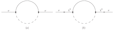
Figure 2: (a) The basic 1–loop diagram giving rise to the Majorana neutrino mass in the $R$-parity violating MSSM. (b) 1–loop diagram with RpV neutrino–neutralino couplings included on the external lines.

The topology of the basic type of 1–loop diagrams we will consider is presented on Fig. 2(a). These diagrams lead to Majorana neutrino mass term, where the effective interaction vertex is expanded into the RpV particle–sparticle loop. These diagrams and their more complicated versions with the Higgs bosons and sneutrinos inside the loop, were classified in e.g. Ref. rpvneutrinos and discussed in details elsewhere (see Haug ; Bhatta ; Abada ; rpvneutrinos ; mg-art6 ; mg-art9 ; mg-art11 ; bounds-3linear among others). In the present paper we add the possible neutrino–neutralino mixing on the external lines (Fig. 2(b)), which leads to another contributions to the neutrino mass. Obviously this additional contribution must be in agreement with the present experimental data. We discuss two main cases, in which either lepton and slepton or quark and squark are in the loop (in the case of higgsino $\tilde{H}_{u}$ only the up-type quarks count). At the same time the neutrino may mix either with the gauginos: bino $\tilde{B}$ or wino $\tilde{W}^{3}$, or with the neutral up-type higgsino $\tilde{H}_{u}$. All the nine cases together with the relevant bi- and trilinear coupling constants have been gathered in Tab. 1.

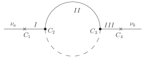
Figure 3: Diagrams with bilinear neutrino–neutralino interactions leading to the Majorana neutrino mass.

Table 1: Nine diagrams with neutrino–neutralino mixing on the external lines leading to Majorana neutrino mass. $I$ and $III$ are the neutralinos which mix with the neutrinos on the external lines of the diagram depicted on Fig. 3. $II$ defines the content of the loop ($u\tilde{u}$ stands for the up-type (s)quarks, $d\tilde{d}$ stands for the down-type (s)quarks,$q\tilde{q}$ for all (s)quarks, and $l\tilde{l}$ for (s)leptons).

	$I$	$II$	$III$	$C_{1}$	$C_{2}$	$C_{3}$	$C_{4}$
1	$\tilde{H}_{u}$	$u\tilde{u}$	$\tilde{H}_{u}$	$\kappa_{a}$	$\sqrt{2}m_{u}/v_{u}$	$\sqrt{2}m_{u}/v_{u}$	$\kappa_{b}$
2	$\tilde{H}_{u}$	$u\tilde{u}$	$\tilde{B}$	$\kappa_{a}$	$\sqrt{2}m_{u}/v_{u}$	$-g^{\prime}/(3\sqrt{2})$	$g^{\prime}\omega_{b}$
3	$\tilde{H}_{u}$	$u\tilde{u}$	$\tilde{W}^{3}$	$\kappa_{a}$	$\sqrt{2}m_{u}/v_{u}$	$-g/\sqrt{2}$	$g\omega_{b}$
4	$\tilde{B}$	$q\tilde{q}$	$\tilde{B}$	$g^{\prime}\omega_{a}$	$-g^{\prime}/(3\sqrt{2})$	$-g^{\prime}/(3\sqrt{2})$	$g^{\prime}\omega_{b}$
5	$\tilde{B}$	$l\tilde{l}$	$\tilde{B}$	$g^{\prime}\omega_{a}$	$-g^{\prime}/\sqrt{2}$	$-g^{\prime}/\sqrt{2}$	$g^{\prime}\omega_{b}$
6a	$\tilde{W}^{3}$	$u\tilde{u}$	$\tilde{W}^{3}$	$g\omega_{a}$	$-g/\sqrt{2}$	$-g/\sqrt{2}$	$g\omega_{b}$
6b	$\tilde{W}^{3}$	$d\tilde{d}$	$\tilde{W}^{3}$	$g\omega_{a}$	$g/\sqrt{2}$	$g/\sqrt{2}$	$g\omega_{b}$
7	$\tilde{W}^{3}$	$l\tilde{l}$	$\tilde{W}^{3}$	$g\omega_{a}$	$g/\sqrt{2}$	$g/\sqrt{2}$	$g\omega_{b}$
8a	$\tilde{B}$	$u\tilde{u}$	$\tilde{W}^{3}$	$g^{\prime}\omega_{a}$	$-g^{\prime}/(3\sqrt{2})$	$-g/\sqrt{2}$	$g\omega_{b}$
8b	$\tilde{B}$	$d\tilde{d}$	$\tilde{W}^{3}$	$g^{\prime}\omega_{a}$	$-g^{\prime}/(3\sqrt{2})$	$g/\sqrt{2}$	$g\omega_{b}$
9	$\tilde{B}$	$l\tilde{l}$	$\tilde{W}^{3}$	$g^{\prime}\omega_{a}$	$g^{\prime}/\sqrt{2}$	$g/\sqrt{2}$	$g\omega_{b}$

The contributions from individual diagrams have been calculated using the same technique as in Refs. mg-art6 ; mg-art9 . In Ref. mg-art9 we have discussed the possible influence of including the quark mixing in the calculations. Here we neglect this effect.

The neutrino mass matrix resulting from the bilinear processes only can be written as the following sum:

$${\cal M}_{ab}=\sum_{i=1}^{9}{\cal M}_{ab}^{i},$$ (26)

where the separate contributions read

$${\cal M}_{ab}^{i}=\frac{1}{16\pi^{2}}\frac{C_{1}C_{2}C_{3}C_{4}}{m_{I}m_{III}}F_{II}.$$ (27)

The masses of the neutralinos $m_{I}$ and $m_{III}$, and the coupling constants have to be taken from Tab. 1. The functions $F$ represent the contributions from the particle–sparticle loops. They read:

$$F_{u\tilde{u}}=\sum_{i,j}\left[3\frac{\sin 2\theta^{j}}{2}m_{u^{i}}f(x_{2}^{ij},x_{1}^{ij})\right],$$ (28)

$$F_{d\tilde{d}}=\sum_{i,j}\left[3\frac{\sin 2\theta^{j}}{2}m_{d^{i}}f(x_{2}^{ij},x_{1}^{ij})\right],$$ (29)

$$F_{q\tilde{q}}=\sum_{i,j}\left[3\frac{\sin 2\theta^{j}}{2}m_{q^{i}}f(x_{2}^{ij},x_{1}^{ij})\right],$$ (30)

$$F_{l\tilde{l}}=\sum_{i,j}\left[\frac{\sin 2\phi^{j}}{2}m_{l^{i}}f(y_{2}^{ij},y_{1}^{ij})\right],$$ (31)

where $\theta^{j}$ and $\phi^{j}$ are the $j$-th squark and slepton mass eigenstates’ mixing angles, respectively. For simplicity we have defined dimensionless quantities $x_{1,2}^{ab}=(m_{q^{a}}/m_{\tilde{q}_{1,2}^{b}})^{2}$, which are the $a$-th quark mass over the $b$-th squark first or second mass eigenstate ratios. An analogous expression involving the lepton and slepton masses has been named $y_{i}^{ab}$. The function coming from integrating over loop momentum is $f(x,y)=[\log(y)/(y-1)-\log(x)/(x-1)]$. The $j$-sums run over all squarks in $F_{u\tilde{u}}$, $F_{d\tilde{d}}$, and $F_{q\tilde{q}}$, and over all sleptons in $F_{l\tilde{l}}$. The $i$-sums count all quarks in $F_{q\tilde{q}}$, up-type quarks only in $F_{u\tilde{u}}$, down-type quarks in $F_{d\tilde{d}}$, and all leptons in $F_{l\tilde{l}}$. The factor 3 in $F_{u\tilde{u}}$, $F_{d\tilde{d}}$, and $F_{q\tilde{q}}$ accounts for summation over quarks’ colors. It is absent in the case of leptons.

We do not discuss the ${\cal M}^{i}$ contributions separately. The reason is that for different cases the couplings $C_{2}$ and $C_{3}$ enter with opposite signs causing cancellations between such terms. Since none of the ${\cal M}^{i}$ can show up without the others, only the full sum Eq. (26) gives a meaningful picture.

V Phenomenological Majorana neutrino mass matrix

The neutrino mass matrix can be constructed from the Pontecorvo–Maki–Nakagawa–Sakata mixing matrix $U_{PMNS}$ under certain assumptions. The matrix $U_{PMNS}$ is usually parameterized by three angles and three (in the case of Majorana neutrinos) phases as follows:

$$U_{PMNS}=\left(\begin{array}[]{ccc}c_{12}c_{13}&s_{12}c_{13}&s_{13}e^{-i\delta}\\ -s_{12}c_{23}-c_{12}s_{23}s_{13}e^{i\delta}&c_{12}c_{23}-s_{12}s_{23}s_{13}e^{i\delta}&s_{23}c_{13}\\ s_{12}s_{23}-c_{12}c_{23}s_{13}e^{i\delta}&-c_{12}s_{23}-s_{12}c_{23}s_{13}e^{i\delta}&c_{23}c_{13}\end{array}\right)\left(\begin{array}[]{ccc}1&0&0\\ 0&e^{i\phi_{2}}&0\\ 0&0&e^{i\phi_{3}}\end{array}\right),$$ (32)

where $s_{ij}\equiv\sin\theta_{ij}$, $c_{ij}\equiv\cos\theta_{ij}$. Three mixing angles $\theta_{ij}$ ($i<j$) vary between 0 and $\pi/2$. The $\delta$ is the CP violating Dirac phase and $\phi_{2}$, $\phi_{3}$ are CP violating Majorana phases. Their values vary between $0$ and $2\pi$. The explicit expression for the phenomenological mass matrix ${\cal M}^{ph}_{\alpha\beta}$ in terms of $m_{i}$, $\theta_{ij}$, $\delta$, $\phi_{2}$, $\phi_{3}$ is given by mg-art9 :

$${\cal M}_{ee} = ~{}~{}c_{13}^{2}\,c_{12}^{2}\,{m_{1}}\,+\,c_{13}^{2}\,s_{12}^{2}\,{m_{2}}\,{e^{-i2\phi_{{}_{2}}}}\,+\,s_{13}^{2}\,{e^{2\,i\delta}}\,{m_{3}}\,{e^{-i2\phi_{{}_{3}}}},$$

$${\cal M}_{e\mu} = -\,c_{12}\,c_{13}\,\left(\,c_{23}\,s_{12}\,+\,c_{12}\,s_{23}\,s_{13}\,{e^{-i\delta}}\,\right){\it{m_{1}}}$$

$$+\,c_{13}\,s_{12}\left(\,c_{23}\,c_{12}\,-\,s_{23}\,s_{12}\,s_{13}\,{e^{-i\delta}}\right)\,{\it{m_{2}}}\,{e^{-i2\phi_{{}_{2}}}}\,+\,c_{13}\,s_{23}\,s_{13}\,{e^{i\delta}}\,{m_{3}}\,{e^{-i2\phi_{{}_{3}}}},$$

$${\cal M}_{e\tau} = -\,c_{12}\,c_{13}\,\left(-\,s_{23}\,s_{12}\,+\,c_{23}\,c_{12}\,s_{13}\,{e^{-i\delta}}\right)\,{m_{1}}$$

$$-\,c_{13}\,s_{12}\,\left(\,c_{12}\,s_{23}\,+\,c_{23}\,s_{12}\,s_{13}\,{e^{-i\delta}}\,\right){m_{2}}{e^{-i2\phi_{{}_{2}}}}\,+\,c_{23}\,c_{13}\,s_{13}\,{e^{i\delta}}\,{m_{3}}\,{e^{-i2\phi_{{}_{3}}}},$$

$${\cal M}_{\mu\mu} = ~{}~{}\left(c_{23}^{2}\,s_{12}^{2}\,+\,2\,c_{23}\,c_{12}\,s_{23}\,s_{12}\,s_{13}\,{e^{-i\delta}}\,+c_{12}^{2}\,s_{23}^{2}\,s_{13}^{2}\,{e^{-2\,\delta}}\right)\,m_{1}\,$$

$$+\left(c_{23}^{2}\,c_{12}^{2}\,-\,2\,c_{23}\,c_{12}\,s_{23}\,s_{12}\,s_{13}\,{e^{-i\delta}}\,+\,s_{23}^{2}\,s_{12}^{2}\,s_{13}^{2}\,{e^{-2\,\delta}}\right)\,{m_{2}}\,{e^{-i2\phi_{{}_{2}}}}\,+\,c_{13}^{2}\,s_{23}^{2}\,{m_{3}}\,{e^{-i2\phi_{{}_{3}}}},$$

$${\cal M}_{\mu\tau} = -\left(c_{23}\,s_{23}\,s_{12}^{2}\,-\,c_{23}^{2}\,c_{12}\,s_{12}\,s_{13}\,{e^{-i\delta}}\,+\,c_{12}\,s_{23}^{2}\,s_{12}\,s_{13}\,{e^{-i\delta}}\,-\,c_{23}\,c_{12}^{2}\,s_{23}\,s_{13}^{2}\,{e^{-2\,i\delta}}\,\right){\it{m_{1}}}$$

$$-\left(c_{23}\,c_{12}^{2}\,s_{23}\,+\,c_{23}^{2}\,c_{12}\,s_{12}\,s_{13}\,{e^{-i\delta}}\,-\,c_{12}\,s_{23}^{2}\,s_{12}\,s_{13}\,{e^{-i\delta}}\,-\,c_{23}\,s_{23}\,s_{12}^{2}\,s_{13}^{2}\,{e^{-2\,i\delta}}\,\right)\,{m_{2}}\,{e^{-i2\phi_{{}_{2}}}}$$

$$\,+\,c_{23}\,c_{13}^{2}\,s_{23}\,{m_{3}}\,{e^{-i2\phi_{{}_{3}}}},$$

$${\cal M}_{\tau\tau} = ~{}~{}\left(s_{23}^{2}\,s_{12}^{2}\,-\,2\,c_{23}\,c_{12}\,s_{23}\,s_{12}\,s_{13}\,{e^{-i\delta}}\,+\,c_{23}^{2}\,c_{12}^{2}\,s_{13}^{2}\,{e^{-2\,i\delta}}\right){m_{1}}$$

$$+\left(c_{12}^{2}\,s_{23}^{2}\,+\,2\,c_{23}\,c_{12}\,s_{23}\,s_{12}\,s_{13}\,{e^{-i\delta}}+c_{23}^{2}\,s_{12}^{2}\,s_{13}^{2}\,{e^{-2\,i\delta}}\right)\,{m_{2}}\,{e^{-i2\phi_{{}_{2}}}}\,+\,c_{23}^{2}\,c_{13}^{2}\,{m_{3}}\,{e^{-i2\phi_{{}_{3}}}}.$$

In order to calculate numerical values of elements of this matrix one needs some additional relations among the mass eigenstates $m_{1,2,3}$. Experiments in which neutrino oscillations are investigated allow to measure the absolute values of differences of neutrino masses squared and the values of the mixing angles. The best-fit values of these parameters read nu-osc ; nu-mass

$$|m_{1}^{2}-m_{2}^{2}| = 7.1\times 10^{-5}\hbox{ eV}^{2},$$

$$|m_{2}^{2}-m_{3}^{2}| = 2.1\times 10^{-3}\hbox{ eV}^{2},$$

$$\sin^{2}(\theta_{12}) = 0.2857,$$ (34)

$$\sin^{2}(\theta_{23}) = 0.5,$$

$$\sin^{2}(\theta_{13}) = 0.$$

The present experimental outcomes are in agreement with two scenarios:

• the normal hierarchy (NH) of masses imply the relation $m_{1}<m_{2}<m_{3}$,

• the inverted hierarchy (IH) of masses imply the relation $m_{3}<m_{1}<m_{2}$.

Notice that in order to keep the same notation for the differences of masses squared and the mixing angles, the neutrino mass eigenstates are labeled differently in the NH and IH cases.

At this point we are left with four undetermined parameters, which are the phases and the mass of the lightest neutrino. To obtain most stringent limits on the new physics parameters the later is taken to be zero. As far as the phases are concerned we consider two separate cases. First we take all possible combinations of phases and for each entry of the matrix we pick up its highest possible value. In this way we obtain unphysical matrices, which give however some idea about the upper limits on the non-standard parameters. The maximal matrices for the NH and IH scenarios read as follows mg-art9 :

$$|\cal{M}|_{\rm max}^{\rm(NH)}\leq\pmatrix{0.00452&0.00989&0.00989\cr 0.00989&0.02540&0.02540\cr 0.00989&0.02540&0.02540}\hbox{ eV},$$ (35)

$$|\cal{M}|_{\rm max}^{\rm(IH)}\leq\pmatrix{0.0452&0.0312&0.0312\cr 0.0312&0.0240&0.0239\cr 0.0312&0.0239&0.0240}\hbox{ eV}.$$ (36)

The more conservative approach assumes that the $CP$ symmetry is preserved which can be achieved by neglecting the phases present in the $U_{PMNS}$ matrix. In such a case the NH and IH matrices take the following forms:

$$|\cal{M}|^{\rm(NH)}=\pmatrix{0.00240&0.00269&0.00269\cr 0.00269&0.02553&0.01951\cr 0.00269&0.01951&0.02553}\hbox{ eV},$$ (37)

$$|\cal{M}|^{\rm(IH)}=\pmatrix{0.045267&0.000249&0.000249\cr 0.000249&0.022801&0.022801\cr 0.000249&0.022801&0.022801}\hbox{ eV}.$$ (38)

Yet another possibility is to construct ${\cal M}$ using constraints from non-observability of the neutrinoless double beta decay ($0\nu 2\beta$). The study of the $0\nu 2\beta$ decay 0n2b is one of the most sensitive ways known to probe the absolute values of neutrino masses and the type of the spectrum. The most stringent lower bound on the half-life of $0\nu 2\beta$ decay were obtained in the Heidelberg-Moscow ⁷⁶Ge experiment H-M ($T^{0\nu-exp}_{1/2}\geq 1.9\times 10^{25}$ yr). By assuming the nuclear matrix element of Ref. FedorVogel we end up with $|m_{\beta\beta}|=U^{2}_{e1}\,m_{1}+U^{2}_{e2}\,m_{2}+U^{2}_{e3}\,m_{3}\leq 0.55\hbox{ eV}$, where $U$ is the neutrino mixing matrix Eq. (32). The element $|m_{\beta\beta}|$ coincides with the $ee$ element of the neutrino mass matrix in the flavor basis and fixing it allows to construct the full maximal matrix, which reads:

$$|{\cal M}|_{\rm max}^{\rm(HM)}\leq\pmatrix{0.55&1.29&1.29\cr 1.29&1.35&1.04\cr 1.29&1.04&1.35}\hbox{ eV}.$$ (39)

In the next section we present the results for each of these five cases.

Table 2: Some results for the SUSY scenario $\tan\beta=10$, $A_{0}=200$, $m_{0}=200\hbox{ GeV}$, $m_{1/2}=500\hbox{ GeV}$.

$\kappa_{1}^{GUT}$	$\kappa_{2}^{GUT}$	$\kappa_{3}^{GUT}$	Resulting mass matrix	Compare with	Remarks
[MeV]			[eV]
$9.50$	$14.80$	$14.80$	$\pmatrix{0.553927&0.864372&0.861090\cr 0.865038&1.349844&1.344714\cr 0.859783&1.341638&1.336555}$	${\cal M}^{\rm(HM)}_{\rm max}$	$\mu\tau$ elements to big
$9.46$	$13.02$	$13.02$	$\pmatrix{0.548762&0.757606&0.753587\cr 0.757853&1.046272&1.040721\cr 0.752398&1.038740&1.033237}$	${\cal M}^{\rm(HM)}_{\rm max}$
$0.85$	$2.03$	$2.03$	$\pmatrix{0.004520&0.010728&0.010698\cr 0.010734&0.025474&0.025404\cr 0.010686&0.025361&0.025292}$	${\cal M}^{\rm(NH)}_{\rm max}$	$e\mu$ and $e\tau$ elements to big
$2.72$	$1.98$	$1.98$	$\pmatrix{0.045316&0.032954&0.032976\cr 0.032945&0.023958&0.023974\cr 0.032951&0.023963&0.023978}$	${\cal M}^{\rm(IH)}_{\rm max}$	$e\mu$ and $e\tau$ elements to big
$0.62$	$2.03$	$2.03$	$\pmatrix{0.002402&0.007824&0.007802\cr 0.007821&0.025474&0.025404\cr 0.007787&0.025361&0.025292}$	${\cal M}^{\rm(NH)}$	$e\mu$, $e\tau$ and $\mu\tau$ elements to big
$0.62$	$0.70$	$0.70$	$\pmatrix{0.002402&0.002691&0.002687\cr 0.002688&0.003011&0.003007\cr 0.002684&0.003007&0.003003}$	${\cal M}^{\rm(NH)}$
$2.72$	$1.92$	$1.93$	$\pmatrix{0.045316&0.032053&0.032118\cr 0.032065&0.022680&0.022726\cr 0.032084&0.022694&0.022740}$	${\cal M}^{\rm(IH)}$	$e\mu$ and $e\tau$ elements to big
$0.27$	$0.19$	$0.19$	$\pmatrix{0.000453&0.000320&0.000321\cr 0.000320&0.000226&0.000227\cr 0.000320&0.000226&0.000227}$	${\cal M}^{\rm(IH)}$

VI Constraining $\kappa$ couplings from the neutrino mass matrix

Figure 4: Allowed parameter space in the maximal HM case.

Figure 5: Allowed parameter space in the maximal NH case.

Figure 6: Allowed parameter space in the maximal IH case.

Figure 7: Allowed parameter space in the NH case with conserved CP symmetry.

Figure 8: Allowed parameter space in the IH case with conserved CP symmetry.

Our aim is to find constraints on the $\kappa_{i}$ coupling constants coming from the neutrino mass matrices. As an example of the unification conditions we take the following input:

$$A_{0}=200,\quad m_{0}=200\hbox{ GeV},\quad m_{1/2}=500\hbox{ GeV},$$ (40)

and additionally

$$\tan\beta=10,\qquad{\rm sgn}(\mu)=1.$$ (41)

We do not expect great differences in the results if the GUT conditions were changed. The only exception may be the $\tan\beta$ parameter (defined at $m_{z}$ scale) which dominates the running of the $\kappa$’s. By looking on Fig. 1 only very low values of this parameter will influence the results significantly.

We proceed in two steps. Firstly we find such values of $\kappa_{i}^{GUT}$ which will reproduce the diagonal elements of the mass matrices. This can be achieved with good accuracy, but it turns out that some of the elements (off-diagonal, see remarks in Tab. 2) of the resulting matrix exceed the allowed values. It means that the $\kappa$’s will not take their maximal values simultaneously.

Secondly we go down with the $\kappa_{i}^{GUT}$ to lower the off-diagonal elements to the acceptable level. This, however, can be done in many different ways. Some explicit examples are listed in Tab. 2 but to find the full allowed parameter space we have prepared scatter plots which are presented on Figs. 4–8. Each of the plots consists of roughly 2000 points chosen randomly from the intervals between zero and 1.1 times the assessed upper limit for given $\kappa_{i}^{GUT}$.

The boundaries of the allowed parameter space for $\kappa_{i}$ in the case of unphysical neutrino mass matrices $|{\cal M}|_{\rm max}^{\rm(HM,NH,IH)}$ are nearly box-shaped, except for a small region of excluded values in the upper right-hand corner of some of the plots. This behavior is expected, as the mass matrices to be reproduced contain on each entry the maximal allowed value for it.

Much more interesting shapes are obtained for the CP conserved cases (Figs. 7 and 8). The projections onto the $(\kappa_{1},\kappa_{2})$ and $(\kappa_{1},\kappa_{3})$ planes are nearly identical and contain non-linear boundary parts. The most constrained is the inverted hierarchy case with conserved CP (Fig. 8) due to two orders of magnitude differences between the diagonal $\mu\mu$ and $\tau\tau$ and off-diagonal $e\mu$ and $e\tau$ elements.

VII The transition magnetic moment

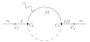
Figure 9: Feynman diagram with neutrino-neutralino mixing on the external lines, leading to the Majorana neutrino transition magnetic moment.

The RpV loop diagrams provide not only an elegant mechanism of generating Majorana neutrino mass terms, but also, after a minor modification, may be the source of the transition magnetic moment $\mu_{ab}$. This quantity represents roughly the strength of the electromagnetic interaction of the neutrino. Since the latter is electrically neutral, the interaction must take place between an external photon and a charged particle from inside the virtual RpV loop. In practice, only the photon–fermion interactions are taken into account, since the photon–boson (squark or slepton) interaction would be strongly suppressed by the big mass of the SUSY particle. The relevant Feynman diagram is presented on Fig. 9.

The contribution to the Majorana neutrino magnetic moment from the discussed diagrams is given by (in Bohr magnetons $\mu_{B}$)

$$\mu_{ab} = (1-\delta_{ab})\frac{m_{e^{1}}}{4\pi^{2}}\ \left(C_{1a}\frac{C_{2}C_{3}}{m_{I}m_{III}}C_{4b}\right)$$ (42)

$$\times \sum_{i,j}\left[3\frac{w_{ij}^{(q)}}{m_{q^{i}}}Q_{q^{i}}+\frac{w_{ij}^{(\ell)}}{m_{\ell^{i}}}Q_{\ell^{i}}\right]\mu_{B}.$$

Here we have denoted the electric charge of a particle (in units of $e$) by $Q$. The dimensionless loop functions $w$ take the forms

$$w_{ij}^{(q)}=\frac{\sin 2\theta^{j}}{2}g(x_{2}^{ij},x_{1}^{ij}),\quad w_{ij}^{(\ell)}=\frac{\sin 2\phi^{j}}{2}g(y_{2}^{ij},y_{1}^{ij}),$$ (43)

where $\theta$, $\phi$, $x_{1,2}$, and $y_{1,2}$ are the same as in Eqs. (28)–(31), and $g(x,y)=(x\log(x)-x+1)(1-x)^{-2}-(x\to y)$. The sum over $i$ and $j$ in Eq. (42) accounts for all the possible quark-squark and lepton-slepton configurations for given neutralinos. The factor 3 in front of $w^{(q)}$ counts the three quark colors.

The results for the already discussed GUT parameters are presented in Tab. 3. The last column contains for comparison upper bounds for the magnetic moment in the case when only trilinear interactions are taken into account. One sees that they are at least one order of magnitude stronger than the discussed bilinear contributions.

Table 3: Contribution to the Majorana neutrino transition magnetic moments coming from the bilinear neutrino-neutralino mixing, for the GUT scenario: $A_{0}=200$, $m_{0}=200\hbox{ GeV}$, $m_{1/2}=500\hbox{ GeV}$, $\tan\beta=10$.

	$\mu_{e\mu}$	$\mu_{e\tau}$	$\mu_{\mu\tau}$	trilinear only
IH-CP	$7.0\times 10^{-22}$	$7.0\times 10^{-22}$	$6.0\times 10^{-20}$	$\leq 10^{-19}$
IH-max	$8.8\times 10^{-20}$	$8.5\times 10^{-20}$	$6.5\times 10^{-20}$	$\leq 10^{-17}$
NH-CP	$7.6\times 10^{-21}$	$7.6\times 10^{-21}$	$5.5\times 10^{-20}$	$\leq 10^{-18}$
NH-max	$2.8\times 10^{-20}$	$2.8\times 10^{-20}$	$7.0\times 10^{-20}$	$\leq 10^{-17}$
HM-max	$2.4\times 10^{-18}$	$2.3\times 10^{-18}$	$2.9\times 10^{-18}$	$\leq 10^{-15}$

Table 4: Like in Tab. 3 but with $A_{0}=100$, $m_{0}=150\ \hbox{ GeV}$, $m_{1/2}=150\ \hbox{ GeV}$, $\tan\beta=19$.

	$\mu_{e\mu}$	$\mu_{e\tau}$	$\mu_{\mu\tau}$	trilinear only
IH-CP	$3.0\times 10^{-21}$	$2.9\times 10^{-21}$	$2.5\times 10^{-19}$	$\leq 10^{-18}$
IH-max	$3.7\times 10^{-19}$	$3.6\times 10^{-19}$	$2.7\times 10^{-19}$	$\leq 10^{-18}$
NH-CP	$3.2\times 10^{-20}$	$3.1\times 10^{-20}$	$2.2\times 10^{-19}$	$\leq 10^{-18}$
NH-max	$1.2\times 10^{-19}$	$1.1\times 10^{-19}$	$2.9\times 10^{-19}$	$\leq 10^{-18}$
HM-max	$1.0\times 10^{-17}$	$9.8\times 10^{-18}$	$1.2\times 10^{-17}$	$\leq 10^{-16}$

Table 5: Like in Tab. 3 but with $A_{0}=500$, $m_{0}=1000\ \hbox{ GeV}$, $m_{1/2}=1000\ \hbox{ GeV}$, $\tan\beta=19$.

	$\mu_{e\mu}$	$\mu_{e\tau}$	$\mu_{\mu\tau}$	trilinear only
IH-CP	$3.7\times 10^{-22}$	$3.7\times 10^{-22}$	$3.3\times 10^{-20}$	$\leq 10^{-20}$
IH-max	$4.6\times 10^{-20}$	$4.6\times 10^{-20}$	$3.5\times 10^{-20}$	$\leq 10^{-20}$
NH-CP	$4.0\times 10^{-21}$	$4.0\times 10^{-21}$	$2.9\times 10^{-21}$	$\leq 10^{-20}$
NH-max	$1.4\times 10^{-20}$	$1.5\times 10^{-20}$	$3.7\times 10^{-20}$	$\leq 10^{-20}$
HM-max	$1.3\times 10^{-18}$	$1.2\times 10^{-18}$	$1.5\times 10^{-18}$	$\leq 10^{-18}$

In Tabs. 4 and 5 we show the results of similar calculations for two other set of parameters. In Tab. 4 the unification parameters are ‘low’, while in Tab. 5 their values are ‘higher’. The last column is given as previously for comparison. Also here the conclusion is clear, that the discussed contribution to the main process is at best of the same order of magnitude, in most cases being at least an order of magnitude weaker. The reason for such a situation is due to the high masses of the neutralinos, which enter the formula Eq. (42) in the denominator. It was possible that they will be compensated by the unknown coupling constants proportional to the sneutrino vacuum expectation values $\omega$, especially that some of them are multiplied by negative numbers, cf. Tab. 2. Our explicit calculation showed that it is not the case. Also the observed differences between the values of $\mu_{ab}$, reaching not more than one order of magnitude, are mainly due to the changed value of the parameter $\tan\beta$, and only partially due to different values of the remaining parameters.

VIII Summary

The $R$-parity violating MSSM has many free parameters which lower its predictive power. On the other hand this fact makes the model very flexible. In this paper we have presented a method of constraining the bilinear RpV couplings $\kappa$.

We have calculated the contributions to the neutrino mass matrix coming from the neutrino–neutralino mixing in processes in which the effective vertex is expanded into a virtual quark–squark or lepton–slepton loop. These contributions have been compared with the phenomenological mass matrices derived using the best-fit experimental values of the neutrino mixing angles and differences of masses squared. We discuss four cases in which normal and inverted hierarchy is explored both with conserved CP symmetry and with maximal values of each matrix element. We also present the fifth case in which the neutrino mass matrix is calculated from the data published by the Heidelberg–Moscow neutrinoless double beta decay experiment.

In general we have found that setting the $\kappa$ couplings at the unification scale to values of the order of $\lesssim{\cal O}(1\hbox{ MeV})$ renders the mass contributions correctly below the experimental upper bound. Another observation is that the bilinear RpV mechanism alone is not sufficient to reproduce the whole mass matrix. This is, however, acceptable because in the general RpV loop mechanism one has to sum up the contributions from the tree–level Haug ,

$${\cal M}^{tree}_{ii^{\prime}}=\Lambda_{i}\Lambda_{i^{\prime}}\ g_{2}^{2}$$ (44)

$$\times\frac{M_{1}+M_{2}\tan^{2}\theta_{W}}{4(\mu m_{W}^{2}(M_{1}+M_{2}\tan^{2}\theta_{W})\sin 2\beta-M_{1}M_{2}\mu^{2})},$$ (45)

(46)

where $\Lambda_{i}=\mu\omega_{i}-v_{d}\kappa_{i}$ are the so-called alignment parameters, as well as contributions coming from the 1–loop diagrams (see Fig. 2(a)), which are proportional to the totally unconstrained trilinear couplings $\lambda$ and $\lambda^{\prime}$. These parameters may be easily fine-tuned to reproduce the full mass matrix and we shift this discussion to an upcoming paper.

The knowledge of the bounds on the $\kappa$ coupling constants allows one to discuss many exotic processes, like the neutrino decay and the interaction of neutrino with a photon, to mention only a few. The former may occur as a two-step process, first through bilinear mixing with neutralinos, and then the decay of the actual neutralino. The later has been presented in the previous section showing by explicit calculation that this contribution does not exceed the main 1–loop mechanism.

In our calculations we have fixed the GUT unification parameters. Due to technical difficulties in performing a full skan over the allowed parameter space we have picked only three representatives for which the calculations were performed. We expect that the results will not change qualitatively with the changes of the input parameters, which is of course an assumption that may be worth checking.

References

• (1) Super-Kamiokande Collaboration: S. Fukuda et al., Phys. Rev. Lett. 81, 1562 (1998); Y. Ashie et al., Phys. Rev. Lett. 93, 101801 (2004); Phys. Rev. D 71, 112005 (2005); KamLAND Collaboration: T. Araki et al., Phys. Rev. Lett. 94, 081801 (2005); SNO Collaboration: Q.R. Ahmed et al., Phys. Rev. Lett. 87, 071301 (2001); Phys. Rev. Lett. 89, 011301 (2002); Phys. Rev. Lett. 89, 011302 (2002); B. Aharmin et al., Phys. Rev. C 72 055502 (2005); CHOOZ Collaboration: M. Apollonio et al., Phys. Lett. B 466, 415 (1999); Eur. Phys. J. C 27, 331 (2003); G.L. Fogli, et al., Phys. Rev. D 66, 093008 (2002).
• (2) H.E. Haber and G.L. Kane, Phys. Rep. 17, 75 (1985).
• (3) C. Aulakh and R. Mohapatra, Phys. Lett. B 119, 136 (1983); G.G. Ross and J.W.F Valle, Phys. Lett. B 151, 375 (1985); J. Ellis et al., Phys. Lett. B 150, 142 (1985); A. Santamaria and J.W.F. Valle, Phys. Lett. B 195, 423 (1987); Phys. Rev. D 39, 1780 (1989); Phys. Rev. Lett. 60, 397 (1988); A. Masiero and J.W.F. Valle, Phys. Lett. B 251, 273 (1990).
• (4) M.A. Diaz, J.C. Romao, and J.W.F. Valle, Nucl. Phys. B 524, 23 (1998); A. Akeroyd et al., Nucl. Phys. B 529,3 (1998); A.S. Joshipura, M. Nowakowski, Phys. Rev. D 51, 2421 (1995); Phys. Rev. D 51, 5271 (1995).
• (5) M. Nowakowski and A. Pilaftsis, Nucl. Phys. B 461, 19 (1996).
• (6) L.J. Hall and M. Suzuki, Nucl. Phys. B 231, 419 (1984); G.G. Ross and J.W.F. Valle, Phys. Lett. B 151, 375 (1985); R. Barbieri, D.E. Brahm, L.J. Hall, and S.D. Hsu, Phys. Lett. B 238, 86 (1990); J.C. Ramao and J.W.F. Valle, Nucl. Phys. B 381, 87 (1992); H. Dreiner and G.G. Ross, Nucl. Phys. B 410, 188 (1993); D. Comelli et al., Phys. Lett. B 234, 397 (1994); G. Bhattacharyya, D. Choudhury, and K. Sridhar, Phys. Lett. B 355, 193 (1995); G. Bhattacharyya and A. Raychaudhuri, Phys. Lett. B 374, 93 (1996); A.Y. Smirnov, F. Vissani, Phys. Lett. B 380, 317 (1996); L.J. Hall and M. Suzuki, Nucl. Phys. B 231, 419 (1984).
• (7) A. Faessler, S. G. Kovalenko, and F. Šimkovic, Phys. Rev. D 58, 055004 (1998); M. Hirsch and J.W.F. Valle, Nucl. Phys. B 557, 60 (1999).
• (8) M. Hirsch, M.A. Diaz, W. Porod, J.C. Romao, and J.W.F. Valle, Phys. Rev. D 62, 113008 (2000).
• (9) G.L. Kane, C. Kolda, L. Roszkowski, and J.D. Wells, Phys. Rev. D 49, 6173 (1994).
• (10) D.R.T. Jones, Phys. Rev. D 25, 581 (1982).
• (11) S.P. Martin and M.T. Vaughn, Phys. Rev. D 50, 2282 (1994).
• (12) M. Góźdź and W.A. Kamiński, Phys. Rev. D 69, 076005 (2004).
• (13) P. Cho, M. Misiak, and D. Wyler, Phys. Rev. D 54, 3329 (1996).
• (14) B.C. Allanach, A. Dedes, and H.K. Dreiner, Phys. Rev. D 60, 056002 (1999).
• (15) B.C. Allanach, A. Dedes, and H.K. Dreiner, Phys. Rev. D 69, 115002 (2004).
• (16) O. Haug, J.D. Vergados, A. Faessler, and S. Kovalenko, Nucl. Phys. B 565, 38 (2000).
• (17) G. Bhattacharyya, H.V. Klapdor-Kleingrothaus, and H. Päs, Phys. Lett. B 463, 77 (1999).
• (18) A. Abada and M. Losada, Phys. Lett. B 492, 310 (2000); Nucl. Phys. B, 585, 45 (2000).
• (19) S. Davidson and M. Losada, Phys. Rev. D 65 075025 (2002); Y. Grossman and S. Rakshit, Phys. Rev. D 69 093002 (2004).
• (20) M. Góźdź, W.A. Kamiński, and F. Šimkovic, Phys. Rev. D 70, 095005 (2004); Int. J. Mod. Phys. E, 15, 441 (2006).
• (21) M. Góźdź, W.A. Kamiński, F. Šimkovic, and A. Faessler, Phys. Rev. D 74 055007 (2006).
• (22) M. Góźdź, W.A. Kamiński, and F. Šimkovic, Acta Phys. Polon. B 37, 2203 (2006).
• (23) B.C. Allanach, A. Dedes, and H.K. Dreiner, Phys. Rev. D 60, 075014 (1999).
• (24) G. Altarelli and F. Feruglio, New J.Phys. 6, 106 (2004), and references therein.
• (25) G. Racah, Nuovo Cim. 14 (1937) 322; J. Schechter and J.W.F. Valle, Phys. Rev. D 25 2951 (1982); I. Ogawa et al., Nucl. Phys. A 730 215 (2004).
• (26) H.V. Klapdor-Kleingrothaus et al., Eur. Phys. J. A 12, 147 (2001).
• (27) V.A. Rodin, A. Faessler, F. Šimkovic, and P. Vogel, Phys. Rev. C 68 (2003) 044302.