Entanglement between an auto-ionization system and a neighbor atom

Abstract

Entanglement between two electrons belonging to an auto-ionization system and a neighbor two-level atom produced by the dipole-dipole interaction is studied. The entanglement is quantified using the quadratic negativity of a bipartite system including the continuum of states. Suitable conditions for the generation of highly entangled states of two electrons are revealed. Internal structure of the entanglement is elucidated using the spectral density of quadratic negativity.

I Introduction

Ionization is a process in which an electron is transferred from its bound discrete state into a continuum of free states, e.g., by interacting with an optical field. In a stationary optical field, an electron at an atom gradually leaves its bound state and moves into an ionized free state Matulewski et al. (2003). This process is irreversible. It can be utilized for the generation of entangled electron states that are stable in time. The time-dependent entanglement among bound electrons can easily be generated in reversible interactions (Coulomb interaction, dipole-dipole interaction). The irreversible ionization can subsequently ’freeze’ it and provide this way the stability in time. We demonstrate this approach on the simplest model of two atoms, one of which allows the electron ionization.

It is well known that the process of ionization is strongly influenced by the presence of additional discrete excited states (auto-ionization levels). They considerably modify the long-time photoelectron ionization spectra (for an extended list of references, see, e.g. Agarwal et al. (1984); Leoński et al. (1987); Leoński and Tanaś (1988); Leoński et al. (1988)). There even might occur Fano zeros Fano (1961); Rzażewski and Eberly (1981); Lambropoulos and Zoller (1981) in the spectra of isolated auto-ionization systems due to the mutual interference of different ionization paths. The interaction of an auto-ionization system with neighbor atoms leads to the presence of dynamical zeros Lukš et al. (2010); Peřina Jr. et al. (2011a, b, c, d) that occur periodically in time. Ionization spectra contain useful information about bound states of an atom and that is why they have widely been studied experimentally Journel et al. (1993). Auto-ionization systems have also been found useful as media exhibiting electromagnetically-induced transparency and slowing down the propagating light Raczyński et al. (2006). The ionization process is also sensitive to quantum properties of the optical field Leoński (1993).

Here, we consider two atoms in a stationary optical field that moves electrons from their ground states into excited or ionized states. Electrons in their excited states mutually interact by the dipole-dipole interaction Silinsh and Čápek (1994). This creates quantum correlations (entanglement) between two electrons. Whereas one electron remains in a bound state, the second one is allowed to be ionized. We pay attention both to the temporal entanglement formation Bouwmeester et al. (2000); Nielsen and Chuang (2000) and its long-time limit. The quadratic negativity of a bipartite system generalized to the continuum of states is used to quantify the entanglement. We show that highly entangled states can be reached in a wide area of parameters characterizing the system of two atoms.

The paper is organized as follows. A semiclassical model of the system under consideration is described in Sec. II together with its the most general solution. The formula for negativity as a measure of entanglement in a bipartite system with the continuum of states is derived in Sec. III and compared with quantum discord. The spectral density of quadratic negativity is introduced in Sec. IV. The dynamics of entanglement as well as its long-time limit are discussed in Sec. V. The spectral entanglement is analyzed in Sec. VI. Conclusions are drawn in Sec. VII. Appendix A is devoted to an alternative derivation of the formula for negativity.

II Semiclassical model of optical excitation of an auto-ionization atom interacting with a neighbor atom

We consider an atom $b$ with one auto-ionizing discrete level that interacts with a neighbor two-level atom $a$ by the dipole-dipole interaction (for the scheme, see Fig. 1).

Figure 1: Sketch of an auto-ionization system $b$ interacting with a two-level atom $a$. Ground states are denoted as $|0\rangle_{a}$ and $|0\rangle_{b}$ whereas symbols $|1\rangle_{a}$, $|1\rangle_{b}$, and $|E\rangle$ stand for the excited states. Dipole moments $\mu_{a}$, $\mu_{b}$, and $\mu$ describe the appropriate interactions. The excited discrete state at atom $a$ ($b$) has energy $E_{a}$ ($E_{b}$), whereas energies $E$ characterize excited states $|E\rangle$ of the continuum. Symbol $V$ describes the Coulomb configurational coupling between the excited states at atom $b$. Constants $J_{ab}$ and $J$ emerge from the dipole-dipole interaction between the atoms $a$ and $b$; $\alpha_{L}$ is the pumping amplitude.

Both atoms are excited by a stationary optical field. This composite system can be described by the Hamiltonian $\hat{H}$,

$$\hat{H}=\hat{H}_{\rm a-i}+\hat{H}_{\rm t-a}+\hat{H}_{\rm trans}.$$ (1)

Here, the Hamiltonian $\hat{H}_{\rm a-i}$ characterizes the auto-ionization atom:

$$\hat{H}_{\rm a-i} = E_{b}|1\rangle_{b}{}_{b}\langle 1|+\int dE\,E|E\rangle\langle E|$$ (2)

$$\mbox{}+\int dE\,\left[V|E\rangle\,{}_{b}\langle 1|+\mbox{H.c.}\right]$$

$$\mbox{}+\left[\mu_{b}\alpha_{L}\exp(-iE_{L}t)|1\rangle_{b}{}_{b}\langle 0|+\mbox{H.c.}\right]$$

$$\mbox{}+\int dE\,\left[\mu\alpha_{L}\exp(-iE_{L}t)|E\rangle{}_{b}\langle 0|+\mbox{H.c.}\right].$$

Energy $E_{b}$ means the energy difference between the ground state $|0\rangle_{b}$ and the excited discrete state $|1\rangle_{b}$ of atom $b$. Similarly, energy $E$ stands for the energy difference between the state $|E\rangle$ in the continuum and the ground state $|0\rangle_{b}$. The Coulomb configurational coupling between the excited states of atom $b$ is described by $V$. The dipole moments between the ground state $|0\rangle_{b}$ of atom $b$ and its excited states are denoted as $\mu$ and $\mu_{b}$. The stationary optical field with its amplitude $\alpha_{L}$ oscillates at frequency $E_{L}$. We assume $\hbar=1$.

The Hamiltonian $\hat{H}_{\rm t-a}$ of the neighbor two-level atom $a$ introduced in Eq. (1) takes on the form:

$$\hat{H}_{\rm t-a}=E_{a}|1\rangle_{a}{}_{a}\langle 1|+\left[\mu_{a}\exp(-iE_{L}t)|1\rangle_{a}{}_{a}\langle 0|+\mbox{H.c.}\right],$$ (3)

where $E_{a}$ means the energy difference between the ground state $|0\rangle_{a}$ and the excited state $|1\rangle_{a}$; $\mu_{a}$ stands for the dipole moment.

The Hamiltonian $\hat{H}_{\rm trans}$ in Eq. (1) characterizes the dipole-dipole interaction between electrons at atoms $a$ and $b$:

$$\hat{H}_{\rm trans} = \left(J_{ab}|1\rangle_{b}{}_{b}\langle 0||0\rangle_{a}{}_{a}\langle 1|+\mbox{H.c.}\right)$$ (4)

$$\mbox{}+\int\,dE\left[J|E\rangle{}_{b}\langle 0|\,|0\rangle_{a}{}_{a}\langle 1|+\mbox{H.c.}\right].$$

In Eq. (4), $J_{ab}$ ($J$) quantifies the dipole-dipole interaction that leads to the excitation from the ground state $|0\rangle_{b}$ into the state $|1\rangle_{b}$ ($|E\rangle$) of atom $b$ at the cost of the decay of atom $a$ from the excited state $|1\rangle_{a}$ into the ground state $|0\rangle_{a}$.

Following the approach of Ref. Peřina Jr. et al. (2011b), a state vector $|\psi\rangle(t)$ of the system at time $t$ can be decomposed as

$$|\psi\rangle(t) = c_{00}(t)|0\rangle_{a}|0\rangle_{b}+c_{10}(t)|1\rangle_{a}|0\rangle_{b}$$ (5)

$$\mbox{}+c_{01}(t)|0\rangle_{a}|1\rangle_{b}+c_{11}(t)|1\rangle_{a}|1\rangle_{b}$$

$$\mbox{}+\int\,dEd_{0}(E,t)|0\rangle_{a}|E\rangle$$

$$\mbox{}+\int\,dEd_{1}(E,t)|1\rangle_{a}|E\rangle$$

using time-dependent coefficients $c_{00}$, $c_{01}$, $c_{10}$, $c_{11}$, $d_{0}(E)$, and $d_{1}(E)$.

These coefficients satisfy a system of differential equations which can be conveniently written in the matrix form:

$$\frac{d}{dt}{\bf c}(t) = -i{\bf A}{\bf c}(t)-i\int\,dE{\bf B}{\bf d}(E,t),$$

$$\frac{d}{dt}{\bf d}(E,t) = -i{\bf B}^{\dagger}{\bf c}(t)-i{\bf K}(E){\bf d}(E,t)$$ (6)

and

$${\bf c}(t)=\left[\begin{array}[]{c}c_{00}(t)\\ c_{10}(t)\\ c_{01}(t)\\ c_{11}(t)\end{array}\right],\hskip 14.22636pt{\bf d}(E,t)=\left[\begin{array}[]{c}d_{0}(E,t)\\ d_{1}(E,t)\end{array}\right].$$ (7)

The matrices ${\bf A}$, ${\bf B}$, and ${\bf K}$ introduced in Eq. (6) are time-independent provided that a basis rotated at the pump-field frequency $E_{L}$ is used:

$${\bf A}=\left[\begin{array}[]{cccc}0&\mu_{a}^{*}\alpha_{L}^{*}&\mu_{b}^{*}\alpha_{L}^{*}&0\\ \mu_{a}\alpha_{L}&\Delta_{a}&J_{ab}^{*}&\mu_{b}^{*}\alpha_{L}^{*}\\ \mu_{b}\alpha_{L}&J_{ab}&\Delta_{b}&\mu_{a}^{*}\alpha_{L}^{*}\\ 0&\mu_{b}\alpha_{L}&\mu_{a}\alpha_{L}&\Delta_{a}+\Delta_{b}\end{array}\right],$$ (12)

(13)

$${\bf B}=\left[\begin{array}[]{cc}\mu^{*}\alpha_{L}^{*}&0\\ J^{*}&\mu^{*}\alpha_{L}^{*}\\ V^{*}&0\\ 0&V^{*}\end{array}\right],$$ (18)

$${\bf K}(E)=\left[\begin{array}[]{cc}E-E_{L}&\mu_{a}^{*}\alpha_{L}^{*}\\ \mu_{a}\alpha_{L}&E-E_{L}+\Delta_{a}\end{array}\right].$$ (21)

Here $\Delta_{a}=E_{a}-E_{L}$ and $\Delta_{b}=E_{b}-E_{L}$ stand for the frequency detunings of discrete excited states with respect to the pump-field frequency.

Contrary to the solution of the model equations found in Peřina Jr. et al. (2011b) we adopt here the most general approach based on algebraic decomposition of dynamical matrices and solution of the corresponding Sylvester equation. We first neglect threshold effects in the ionization, eliminate continuum coefficients ${\bf d}(E)$ in Eq. (6), and introduce a new matrix ${\bf M}$:

$${\bf M}={\bf A}-i\pi{\bf B}{\bf B}^{\dagger}.$$ (22)

The matrix ${\bf M}$ describes the dynamics of only discrete states that is governed by the vector ${\bf c}$. We denote eigenvalues of the matrix ${\bf K}(E)$ as $E-\xi_{1}$ and $E-\xi_{2}$ and eigenvalues of the matrix ${\bf M}$ as $\Lambda_{{\bf M}j}$, $j=1,2,3,4$. These eigenvalues occur in the matrix decompositions of matrices ${\bf K}$ and ${\bf M}$:

$${\bf K}(E) = (E-\xi_{1}){\bf K}_{1}+(E-\xi_{2}){\bf K}_{2},$$ (23)

$${\bf M} = \sum_{j=1}^{4}\Lambda_{{\bf M}j}{\bf M}_{j}.$$ (24)

The basis matrices ${\bf K}_{1}$ and ${\bf K}_{2}$ can be obtained from the following equations:

$${\bf K}_{1}+{\bf K}_{2} = {\bf I_{2}},$$

$$(E-\xi_{1}){\bf K}_{1}+(E-\xi_{2}){\bf K}_{2} = {\bf K}(E).$$ (25)

The eigenvalues $\xi_{1}$ and $\xi_{2}$ are given as follows:

$$\xi_{1,2} = E_{L}-\frac{\Delta_{a}\pm\delta\xi}{2},$$

$$\delta\xi = \sqrt{\Delta_{a}^{2}+4|\mu_{a}\alpha_{L}|^{2}}.$$ (26)

Symbol $\delta\xi$ means the frequency of Rabi oscillations of the two-level atom $a$.

Similarly, the basis matrices ${\bf M}_{j}$, $j=1,2,3,4$, arise as the solution of the following equations:

$$\sum_{j=1}^{4}{\bf M}_{j} = {\bf I_{4}},$$

$$\sum_{j=1}^{4}\Lambda_{{\bf M}j}^{k}{\bf M}_{j} = {\bf M}^{k},\hskip 14.22636ptk=1,2,3.$$ (27)

In Eqs. (25) and (27), ${\bf I_{2}}$ and ${\bf I_{4}}$ are $2\times 2$ and $4\times 4$ unit matrices, respectively.

After the introduction of matrix ${\bf M}$ in Eq. (22), the solution of Eqs. (6) for the vector ${\bf c}$ can be written in the very simple form:

$${\bf c}(t)=\exp(-i{\bf M}t){\bf c}(0);$$ (28)

${\bf c}(0)$ is the vector of initial conditions.

On the other hand, a newly introduced matrix ${\bf T}(E)$ (of dimension $2\times 4$) obtained as the solution to the Sylvester equation Gantmacher (2000)

$${\bf K}(E){\bf T}(E)-{\bf T}(E){\bf M}={\bf B}^{\dagger}$$ (29)

is useful for expressing the solution of Eqs. (6) for the continuum of states described by the vector ${\bf d}(E)$. On using the matrix decompositions written in Eqs. (23) and (24), the solution of the Sylvester equation (29) can be expressed as follows:

$${\bf T}(E)=\sum_{k=1}^{2}\sum_{j=1}^{4}\frac{1}{E-\xi_{k}-\Lambda_{{\bf M}j}}{\bf K}_{k}{\bf B}^{\dagger}{\bf M}_{j}.$$ (30)

The components of amplitude spectrum of an ionized electron at atom $b$ are given by the coefficients in the vector ${\bf d}(E,t)$. They can be written in the most general form

$${\bf d}(E,t)=\Bigl{(}\exp[-i{\bf K}(E)t]{\bf T}(E)-{\bf T}(E)\exp[-i{\bf M}t]\Bigr{)}{\bf c}(0)$$ (31)

depending on the initial conditions. We have assumed that $d_{0}(E,0)=d_{1}(E,0)=0$ in the derivation of Eq. (31).

As the interaction processes between the discrete states and the continuum of states are irreversible, the eigenvalues of matrix ${\bf M}$ are complex with negative imaginary parts. As a consequence, the expression in Eq. (31) for the amplitude spectral components ${\bf d}$ simplifies in the long-time limit:

$${\bf d^{lt}}(E,t)=\exp[-i{\bf K}(E)t]{\bf T}(E){\bf c}(0).$$ (32)

III Negativity of a bipartite system in discrete and continuous Hilbert spaces

We need to quantify the amount of entanglement between the two-level atom $a$ and the auto-ionization atom $b$ that has a continuous spectrum. The philosophy based on declinations of the partially-transposed statistical operators of entangled states from the positive-semidefinite partially-transposed statistical operators of separable states Hill and Wootters (1997); Vidal and Werner (2002) has been found fruitful here and has resulted in the definition of negativity.

Following the approach by Hill and Wooters Hill and Wootters (1997), we write a matrix ${\bf P}$ of the statistical operator describing an electron at atom $a$ and a (fully) ionized electron at atom $b$ in a given time $T$ [$d_{j}(E)\equiv d_{j}(E,T)$, $j=0,1$]:

$${\bf P}=\left[\begin{array}[]{cc}d_{0}(E)d_{0}^{*}(E^{\prime})&d_{0}(E)d_{1}^{*}(E^{\prime})\\ d_{1}(E)d_{0}^{*}(E^{\prime})&d_{1}(E)d_{1}^{*}(E^{\prime})\end{array}\right].$$ (33)

We note that the frequencies $E$ and $E^{\prime}$ in Eq. (33) are considered as continuous indices of the matrix ${\bf P}$.

A partially-transposed matrix ${\bf P^{Ta}}$ transposed with respect to the indices of two-level atom $a$ is obtained after the exchange of sub-matrices in the upper-left and lower-right corners of the matrix ${\bf P}$ in Eq. (33):

$${\bf P^{Ta}}=\left[\begin{array}[]{cc}d_{0}(E)d_{0}^{*}(E^{\prime})&d_{1}(E)d_{0}^{*}(E^{\prime})\\ d_{0}(E)d_{1}^{*}(E^{\prime})&d_{1}(E)d_{1}^{*}(E^{\prime})\end{array}\right].$$ (34)

In order to determine negativity $N$, we need to find the eigenvalues $\lambda$ of matrix ${\bf P^{Ta}}$ first. An eigenvalue $\lambda$ together with its eigenvector $(u_{0}(E),u_{1}(E))$ fulfil the following system of equations with a continuous index $E$:

$$d_{0}(E)\int\,dE^{\prime}d_{0}^{*}(E^{\prime})u_{0}(E^{\prime})\hskip 56.9055pt$$

$$\mbox{}+d_{1}(E)\int\,dE^{\prime}d_{0}^{*}(E^{\prime})u_{1}(E^{\prime}) = \lambda u_{0}(E),$$

$$d_{0}(E)\int\,dE^{\prime}d_{1}^{*}(E^{\prime})u_{0}(E^{\prime})\hskip 56.9055pt$$

$$\mbox{}+d_{1}(E)\int\,dE^{\prime}d_{1}^{*}(E^{\prime})u_{1}(E^{\prime}) = \lambda u_{1}(E).$$

Integrals in Eqs. (LABEL:24) give the coefficients $a_{jk}$ of the decomposition of eigenvector functions $u_{j}(E)$ in the basis $d_{j}(E)$:

$$a_{jk}=\int\,dE^{\prime}d_{j}^{*}(E^{\prime})u_{k}(E^{\prime}),\hskip 14.22636ptj,k=0,1.$$ (36)

Using the coefficients $a_{jk}$ defined in Eq. (36), the equations in (LABEL:24) can be rewritten as follows:

$$d_{0}(E)a_{00}+d_{1}(E)a_{01} = \lambda u_{0}(E),$$

$$d_{0}(E)a_{10}+d_{1}(E)a_{11} = \lambda u_{1}(E).$$ (37)

The projection of equations in Eq. (37) onto the basis vectors $d_{j}(E)$ results in a system of four algebraic equations for the coefficients $a_{jk}$ determining the eigenvector $(u_{0}(E),u_{1}(E))$:

$$\left[\begin{array}[]{cccc}b_{00}&b_{01}&0&0\\ 0&0&b_{00}&b_{01}\\ b_{10}&b_{11}&0&0\\ 0&0&b_{10}&b_{11}\end{array}\right]\left[\begin{array}[]{c}a_{00}\\ a_{01}\\ a_{10}\\ a_{11}\end{array}\right]=\lambda\left[\begin{array}[]{c}a_{00}\\ a_{01}\\ a_{10}\\ a_{11}\end{array}\right].$$ (38)

The coefficients $b_{jk}$ introduced in Eq. (38) are the overlap integrals between the functions $d_{0}(E)$ and $d_{1}(E)$:

$$b_{jk}=\int\,dEd_{j}^{*}(E)d_{k}(E).$$ (39)

It holds that $b_{01}=b_{10}^{*}$ and $b_{00}+b_{11}=1$ due to the normalization.

The system of algebraic equations (38) has a nontrivial solution provided that the eigenvalues $\lambda$ are solutions of the secular equation:

$$\lambda^{4}-\lambda^{3}+{\cal D}\lambda-{\cal D}^{2}=0,$$ (40)

where

$${\cal D}=b_{00}b_{11}-b_{01}b_{10}.$$ (41)

The fourth-order polynomial in Eq. (40) can be written as a product of the second-order polynomials $(\lambda^{2}-{\cal D})(\lambda^{2}-\lambda+{\cal D})$. This allows to find its roots:

$$\lambda_{1,2} = \pm\sqrt{\cal D},$$

$$\lambda_{3,4} = \frac{1}{2}\pm\sqrt{\frac{1}{4}-{\cal D}}.$$ (42)

As the negativity $N$ is given by the amount of negativeness in the eigenvalues $\lambda$, we have

$$N=\sqrt{\cal D}.$$ (43)

Alternative and more intuitive derivation of the formula in Eq. (43) can be found in Appendix A invoking the decomposition of functions $d_{0}(E)$ and $d_{1}(E)$.

In parallel to the entanglement, quantum discord Ollivier and Zurek (2001) has been discussed in the last years for systems composed of several parts Al-Qasimi and James (2011). Discord quantifies the amount of information in the whole system that cannot be extracted using quantum measurements at separated parts. Provided that a bipartite system is in a pure state quantum discord is quantified by entropy $S$ of entanglement. The entropy $S$ of entanglement is given by the entropy of reduced statistical operator $\varrho^{a}$ of atom $a$ that takes the form

$$\varrho^{a}=\left[\begin{array}[]{cc}b_{00}&b_{10}\\ b_{01}&b_{11}\end{array}\right]$$ (44)

exploiting the coefficients $b_{jk}$. The eigenvalues $\lambda_{3,4}$ written in Eq.(42) naturally give also the eigenvalues of matrix $\varrho^{a}$ and so they can be conveniently used in expressing the entropy $S$. The entropy $S$ of entanglement is given by the usual formula $S=-\sum_{j=3,4}\lambda_{j}\log_{2}(\lambda_{j})$, $\log_{2}$ being the logarithm of base two. This formula provides us the following expression:

$$S = -\frac{1}{2}\left[\log_{2}({\cal D})+\sqrt{1-4{\cal D}}\log_{2}\left(\frac{1+\sqrt{1-4{\cal D}}}{1-\sqrt{1-4{\cal D}}}\right)\right].$$

Here, determinant ${\cal D}$ of the matrix $\varrho^{a}$ is given in Eq. (41).

Combining Eqs. (43) and (LABEL:34), the entropy $S$ of entanglement can be expressed as a monotonous function of negativity $N$ (see Fig. 2):

$$S = -\log_{2}(N)-\frac{\sqrt{1-4N^{2}}}{2}\log_{2}\left(\frac{1+\sqrt{1-4N^{2}}}{1-\sqrt{1-4N^{2}}}\right).$$

The curve in Fig. 2 reveals that both quantities can be equally well used for the quantification of entanglement in the considered system.

Figure 2: Entropy $S$ of entanglement as a function of negativity $N$ in the interval $[0,0.5]$ of attainable values of $N$.

The negativity $N$ can also be expressed in terms of eigenvalues of the Schmidt decomposition of the state $|\psi\rangle$ in the long-time limit. Substituting Eq. (41) into Eq. (43), we arrive at the useful formula for negativity $N$:

$$N=\sqrt{\frac{1}{2}\sum_{j,k=0}^{1}\left[b_{jj}b_{kk}-b_{jk}b_{kj}\right]}.$$ (47)

Further substitution for the coefficients $b_{jk}$ from Eq. (39) provides the negativity $N$ depending on the reduced statistical operator $\varrho^{b}$ of the continuum:

$$N = \sqrt{\frac{1}{2}\left[1-\int dE\,\int dE^{\prime}\,|\varrho^{b}(E,E^{\prime})|^{2}\right]},\,\,\,$$ (48)

$$\varrho^{b}(E,E^{\prime}) = \sum_{k=0,1}d_{k}(E)d_{k}^{*}(E^{\prime}).$$ (49)

Using the coefficients $\sqrt{\lambda_{3}}$ and $\sqrt{\lambda_{4}}$ of the Schmidt decomposition of the state $|\psi\rangle$, the formula (48) can be recast into the simple form:

$$N=\sqrt{\lambda_{3}\lambda_{4}}.$$ (50)

The formula for negativity $N$ in Eq. (43) can even be used for finite times $t$, in which discrete states of atom $b$ are populated. In this case, the formula in Eq. (39) has to be replaced by the more general one:

$$b_{jk}=\sum_{l}c^{*}_{jl}c_{kl}+\int\,dEd_{j}^{*}(E)d_{k}(E).$$ (51)

IV Quadratic negativity and its spectral density

The substitution of expression in Eq. (41) into the formula (43) for negativity $N$ gives us an expression that indicates the existence of quadratic negativity $N_{q}$ as a measure of entanglement that allows to introduce a spectral density Dür et al. (1999):

$$N_{q}\equiv 4N^{2}=4(b_{00}b_{11}-b_{01}b_{10}).$$ (52)

The use of expressions (39) for the coefficients $b_{jk}$ allows us to rewrite the formula in Eq.(52) as:

$$N_{q}=2\int dE\,\varrho(E)\int\,dE^{\prime}\varrho(E^{\prime})n_{q}(E,E^{\prime}),$$ (53)

where $\varrho(E)$ gives the density of states $|E\rangle$ in the continuum:

$$\varrho(E)=\sum_{j=0}^{1}|d_{j}(E)|^{2}.$$ (54)

The spectral density $n_{q}(E,E^{\prime})$ of quadratic negativity introduced in Eq. (53) is obtained in the form:

$$n_{q}(E,E^{\prime}) = \frac{1}{\varrho(E)\varrho(E^{\prime})}\left[\sum_{j,k=0}^{1}|d_{j}(E)|^{2}|d_{k}(E^{\prime})|^{2}\right.$$ (55)

$$\left.\mbox{}-\sum_{j,k=0}^{1}d^{*}_{j}(E)d_{k}(E)d^{*}_{k}(E^{\prime})d_{j}(E^{\prime})\right].$$

The value of spectral density $n_{q}(E,E^{\prime})$ of quadratic negativity gives the value of quadratic negativity of a qubit-qubit system composed of the states $\{|0\rangle_{a},|1\rangle_{a}\}$ and $\{|E\rangle,|E^{\prime}\rangle\}$. According to Eq. (53), the quadratic negativity $N_{q}$ is given as a weighted sum of quadratic qubit-qubit negativities between the two-level atom $a$ and all possible qubits embedded inside the continuum. This interpretation is important from the physical point of view, because it allows to interpret the overall entanglement as composed of individual spectral contributions. We note that values of both the quadratic negativity $N_{q}$ and its density $n_{q}$ lie in the interval $[0,1]$. We also note that an alternative normalization in the definition (55) of density $n_{q}$ of quadratic negativity is possible. It is based on substituting the factor $1/[\varrho(E)\varrho(E^{\prime})]$ by the factor $4/[\varrho(E)+\varrho(E^{\prime})]^{2}$. However, this ’mathematically more compact’ normalization is not suitable for indicating entanglement in the case of qubits with considerably different values of the probability densities $\varrho(E)$ and $\varrho(E^{\prime})$.

Experimental determination of the density $n_{q}$ of quadratic negativity has to take into account a finite resolution $\Delta E$ of frequencies of free electrons. That is why, it is convenient to introduce a series of experimental quadratic negativities $N_{q}^{(i)}$, $i=1,2,\ldots$, that are obtained after spectral filtering of a free electron by using $i$ filters positioned at the central frequencies $E_{k}$, $k=1,\ldots,i$:

$$N^{(i)}_{q}(E_{1},\ldots,E_{i}) =$$ (56)

$$\Bigl{[}b_{00}^{(i)}(E_{1},\ldots,E_{i})b_{11}^{(i)}(E_{1},\ldots,E_{i})-|b_{01}^{(i)}(E_{1},\ldots,E_{i})|^{2}\Bigr{]}^{1/2}$$

$$\mbox{}\times\Bigl{[}b_{00}^{(i)}(E_{1},\ldots,E_{i})+b_{11}^{(i)}(E_{1},\ldots,E_{i})\Bigr{]}^{-1}.$$

The coefficients $b_{jk}^{(i)}(E_{1},\ldots,E_{i})$ occurring in Eq. (56) depend on the experimental frequency width $\Delta E$ and are given as:

$$b_{jk}^{(i)}(E_{1},\ldots,E_{i})=\sum_{l=1}^{i}\int_{E_{l}-\Delta E/2}^{E_{l}+\Delta E/2}\,dE^{\prime}d_{j}^{*}(E^{\prime})d_{k}(E^{\prime}).$$ (57)

We note that the last term in the expression (56) originates in the normalization of the considered state.

V Entanglement generation

The entanglement between electrons at atoms $a$ and $b$ is generated by the dipole-dipole interaction that is characterized by the coefficients $J_{ab}$ and $J$. This means that two different channels of the entanglement generation exist. In the first channel, the entanglement among the discrete states at atoms $a$ and $b$ is formed due to the dipole-dipole interaction described by the coefficient $J_{ab}$ first. Subsequently, this entanglement is transferred to the continuum of states $|E\rangle$ using either the Coulomb interaction ($V$) or the optical dipole interaction ($\mu\alpha_{L}$). The second channel is based on the dipole-dipole interaction ($J$) between the excited discrete state $|1\rangle_{a}$ at atom $a$ and the continuum of states $|E\rangle$ at the ionization atom $b$.

The dynamics of the system is such that an electron at atom $b$ gradually ’leaks’ into the continuum of states $|E\rangle$. The probability of finding this electron in a combination of discrete states $|0\rangle_{b}$ and $|1\rangle_{b}$ decreases roughly exponentially. After a sufficiently long time, this probability is practically zero, the electron is fully ionized and its long-time spectrum completely characterizes its state. On the other hand, the electron at atom $b$ periodically oscillates between its discrete states in a stationary optical field at the Rabi frequency. The entanglement between the bound electron at atom $a$ and the ionized electron at atom $b$ is formed during the period of ionization and is ’frozen’ as soon as atom $b$ is completely ionized. At this instant, the entanglement reaches its long-time limit, but superimposed periodic oscillations are possible under certain conditions (see below).

Let us concentrate on the first channel. Both electrons at atoms $a$ and $b$ being initially in their ground states gradually move into their excited states $|1\rangle_{a}|0\rangle_{b}$, $|0\rangle_{a}|1\rangle_{b}$, and $|1\rangle_{a}|1\rangle_{b}$ due to the interaction with the stationary optical field [see Fig. 3(a)]. The entanglement between discrete states arises from the dipole-dipole interaction between the states $|1\rangle_{a}|0\rangle_{b}$ and $|0\rangle_{a}|1\rangle_{b}$. The probabilities $|c_{10}|^{2}$ and $|c_{01}|^{2}$ affiliated to these states periodically return to zero with a period that decreases with the increasing values of $|J_{ab}|$, $|\mu_{a}\alpha_{L}|$, and $|\mu_{b}\alpha_{L}|$. At these instants, highly entangled states occur and their quadratic negativities $N_{q}^{d}$ quantifying entanglement among discrete states reach local maxima [see Fig. 3(b)]. Provided that the probabilities of the ground state $|0\rangle_{a}|0\rangle_{b}$ and the state with both electrons excited are balanced ($|c_{00}|^{2}\approx|c_{11}|^{2}$), the quadratic negativity $N_{q}^{d}$ reaches its maximum value one. The quadratic negativity $N_{q}^{d}$ oscillates between its maximum and zero during the time evolution. The entanglement between the discrete states at atom $a$ and the continuum of states at atom $b$ arises as a consequence of the interaction of the continuum of states $|E\rangle$ with the discrete states $|0\rangle_{b}$ and $|1\rangle_{b}$. The quadratic negativity $N_{q}$ appropriate for this entanglement typically increases during the time evolution and gradually reaches its long-time value, as documented in Fig. 3(b). However, weak oscillations may occur in this evolution. The overall quadratic negativity $N_{q}^{f}$ that characterizes the entanglement between atoms $a$ and $b$ including all states, behaves similarly as the quadratic negativity $N_{q}$ comprising only the continuum of states. As a rule of thumb, a slightly stronger optical pumping of atom $a$ compared to atom $b$ ($\mu_{a}>\mu_{b}$) results in greater values of the long-time quadratic negativity $N_{q}^{\rm lt}$.

(a)

(b)

Figure 3: Temporal evolution of (a) probabilities $|c_{00}|^{2}$ (solid curve with $\ast$), $|c_{10}|^{2}$ (solid curve with $\diamond$), $|c_{01}|^{2}$ (solid curve with $\triangle$), $|c_{11}|^{2}$ (solid curve with $\circ$) of detecting two electrons in the appropriate discrete states and their sum $\Sigma$ ($\Sigma=\sum_{j=0,1}\sum_{k=0,1}|c_{jk}|^{2}$, solid curve) and (b) quadratic negativities $N_{q}$ (solid curve with $\ast$), $N_{q}^{f}$ (solid curve with $\triangle$), and $N_{q}^{d}$ (solid curve); $\mu_{a}\alpha_{L}=\mu_{b}\alpha_{L}=J_{ab}=V=0.05$, $\mu=J=0$, $E_{a}=E_{b}=E_{L}=1$.

In the second channel, the entanglement is generated directly by the dipole-dipole interaction between the excited state $|1\rangle_{a}$ and the continuum of states $|E\rangle$. The ability to generate the entanglement is weaker compared to the first channel. ’Transfer of entanglement’ can be observed also here and so nonzero values of the quadratic negativity $N_{q}^{d}$ are found during the temporal evolution [see Fig. 4]. Even the maximum entangled discrete states ($N_{q}^{d}=1$) can be reached. This clearly shows that there exists a strong ’back-action’ from the ’reservoir’ continuum of states $|E\rangle$ towards the discrete states $|0\rangle_{b}$ and $|1\rangle_{b}$. Otherwise, the observed temporal evolution is qualitatively similar to that found in the first channel.

Figure 4: Temporal evolution of quadratic negativities $N_{q}$ (solid curve with $\ast$), $N_{q}^{f}$ (solid curve with $\triangle$), and $N_{q}^{d}$ (solid curve); $J=0.05$, $J_{ab}=0$, values of the other parameters are the same as in the caption to Fig. 3.

Some general features of the behavior of quadratic negativity $N_{q}$ in the long-time limit can be obtained even analytically. A detailed analysis of the long-time solution in Eq. (32) has shown Peřina Jr. et al. (2011b) that the coefficients $b_{00}$ and $b_{11}$ giving the probabilities of finding an electron at atom $a$ in the states $|0\rangle_{a}$ and $|1\rangle_{a}$, respectively, can be expressed in the form:

$$b_{00}^{\rm lt}(t) = a+\left[b\exp(i\delta\xi t)+\mbox{c.c.}\right],$$

$$b_{11}^{\rm lt}(t) = (1-a)-\left[b\exp(i\delta\xi t)+\mbox{c.c.}\right].$$ (58)

Constant $a$ describes the steady-state parts of probabilities $b_{00}$ and $b_{11}$, whereas constant $b$ gives the amount of probability that oscillates between the states $|0\rangle_{a}$ and $|1\rangle_{a}$ at the Rabi frequency $\delta\xi$. The symbol ${\rm c.c.}$ replaces a complex conjugate term. On the other hand, the cross-correlation coefficient $b_{01}$ can be written as

$$b_{01}(t)=c_{1}+c_{2}\exp(i\delta\xi t)+c_{3}\exp(-i\delta\xi t);$$ (59)

$c_{1}$, $c_{2}$, and $c_{3}$ being constants.

Using the equality $b^{2}=-c_{2}c_{3}^{*}$ valid in the model, we arrive at the following formula for the long-time quadratic negativity $N_{q}^{\rm lt}$:

$$N_{q}^{\rm lt}(t) = 4\left\{a(1-a)-2|b|^{2}-|c_{1}|^{2}-|c_{2}|^{2}-\frac{|b|^{4}}{|c_{2}|^{2}}\right.$$ (60)

$$\left.\mbox{}+\left[(1-2a)b-c_{1}^{*}c_{2}+\frac{c_{1}b^{2}}{c_{2}}\right]\exp(i\delta\xi t)\right\}.$$

We can see from Eq. (60) that the quadratic negativity $N_{q}^{\rm lt}$ is composed of a steady-state part and an oscillating part with the Rabi frequency $\delta\xi$. However, the oscillating part is usually much smaller than the steady-state one. Even if atom $a$ is resonantly pumped, the oscillating term in Eq. (60) vanishes and we arrive at the simplified formula:

$$N_{q}^{\rm lt,res}=4\left[a(1-a)-2|b|^{2}-|c_{1}|^{2}-|c_{2}|^{2}-\frac{|b|^{4}}{|c_{2}|^{2}}\right].$$ (61)

According to Eq. (61), equal steady-state probabilities $a$ and $(1-a)$ of detecting the electron at atom $a$ in the states $|0\rangle_{a}$ and $|1\rangle_{a}$, respectively, are needed to reach the maximum value of quadratic negativity $N_{q}^{\rm lt}$ ($a=1/2$). Moreover, nonzero values of constants $|b|$, $|c_{1}|$ and $|c_{2}|$ lower the values of long-time quadratic negativity $N_{q}^{\rm lt}$.

The numerical analysis of the long-time behavior of quadratic negativity $N_{q}^{\rm lt}$ has revealed that the larger the values of dipole-dipole constants $J_{ab}$ and $J$ are, the larger is the potential to generate highly entangled states. In order to arrive at high values of the quadratic negativity $N_{q}^{\rm lt}$, the values of constants $\mu\alpha_{L}$ and $V$ have to be sufficiently small compared to the values of $J$ and $J_{ab}$. This can be physically explained as follows. The constants $\mu\alpha_{L}$ and $V$ determine the speed of transfer of an electron at atom $b$ into the continuum of states $|E\rangle$. If this speed is too fast, the electron at atom $b$ has not enough time to create the entanglement with the electron at atom $a$. As a consequence, the entanglement between two electrons is weaker. This behavior is documented in Fig. 5 considering both channels of entanglement generation. However, the graphs in Fig. 5 reveal that also greater values of the constants $\mu\alpha_{L}$ and $V$ allow to reach strong entanglement under the condition $\mu\alpha_{L}\approx V$. The analysis of temporal behavior of the system has shown that the movement of the electron at atom $b$ into the continuum of states $|E\rangle$ is considerably slowed down in this case of balanced interactions $\mu\alpha_{L}$ and $V$. This slowing-down then gives enough time for the entanglement generation even for smaller values of the constants $J_{ab}$ and $J$. This regime is even preferred for the channel exploiting the constant $J$, as the graph in Fig. 5(b) shows.

(a)

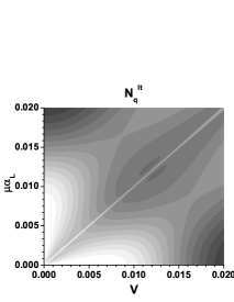
(b)

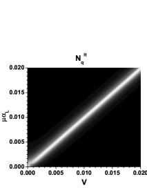
(c)

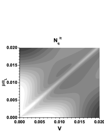
Figure 5: Topo graphs of long-time quadratic negativity $N_{q}^{\rm lt}$ depending on optical pumping $\mu\alpha_{L}$ and strength $V$ of the Coulomb interaction for (a) $J_{ab}=0.001$, $J=0$, (b) $J_{ab}=0$, $J=0.001$, and (c) $J_{ab}=J=0.001$; $\mu_{a}\alpha_{L}=\mu_{b}\alpha_{L}=0.05$, $E_{a}=E_{b}=E_{L}=1$.

Two channels based on the constants $J_{ab}$ and $J$ mutually ’interfere’ in creating the entanglement between two electrons. This can be conveniently used for reaching greater values of the quadratic negativity $N_{q}^{\rm lt}$ in regions, where the above described conditions are not met. Great values of the quadratic negativity $N_{q}^{\rm lt}$ can be obtained in specific areas of the space spanned by the constants $J_{ab}$ and $J$, as illustrated in Fig. 6.

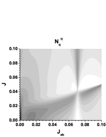
Figure 6: Topo graphs of long-time quadratic negativity $N_{q}^{\rm lt}$ as it depends on dipole-dipole coupling constants $J_{ab}$ and $J$; $\mu_{a}\alpha_{L}=\mu_{b}\alpha_{L}=\mu\alpha_{L}=0.05$, $V=0.01$, $E_{a}=E_{b}=E_{L}=1$.

We have considered the resonant pumping of atoms $a$ and $b$ up to now. The non-resonant pumping of both atoms makes the dynamics as well as the entanglement generation even more complex. Upon depending on conditions, the frequency detuning of atoms $a$ and $b$ may either support the entanglement creation or degrade it. A typical graph showing the behavior of quadratic negativity $N_{q}^{\rm lt}$ in dependence on the detunings $\Delta_{a}$ and $\Delta_{b}$ is plotted in Fig. 7.

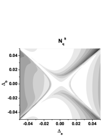
Figure 7: Topo graph of long-time quadratic negativity $N_{q}^{\rm lt}$ as a function of detunings $\Delta_{a}$ and $\Delta_{b}$ of atoms $a$ and $b$, respectively; $\mu_{a}\alpha_{L}=\mu_{b}\alpha_{L}=0.05$, $\mu\alpha_{L}=0.005$, $J_{ab}=V=0.001$, $J=0$, $E_{L}=1$.

VI Spectral entanglement

We illustrate typical properties of the spectral entanglement considering the system characterized by parameters mentioned in the caption to Fig. 3. In Fig. 8, the spectral density $n_{q}$ of quadratic negativity is plotted in the range of relative frequencies that covers two complex peaks occurring in the ionization spectrum (shown in Fig. 18). Strong spectral correlations inside the complex peaks as well as between different peaks are clearly visible. They mainly occur in spectral regions where the fast intensity variations occur (compare Figs. 8 and 9).

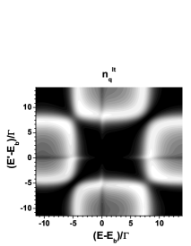
Figure 8: Topo graph of density $n^{\rm lt}_{q}$ of quadratic negativity showing qubit-qubit correlations in relative frequencies $(E-E_{b})/\Gamma$ and $(E^{\prime}-E_{b})/\Gamma$, values of parameters given in the caption to Fig. 3 are used.

Figure 9: Long-time photoelectron ionization spectrum $I^{\rm lt}$; values of parameters given in the caption to Fig. 3 are used.

The experimental quadratic negativity $N_{q}^{(1)}$ defined in Eq. (56) represents the simplest experimentally accessible characteristics. As its definition indicates, the negativity $N_{q}^{(1)}$ depends on the experimental frequency resolution $\Delta E$. It even holds that $N_{q}^{(1)}(E)\rightarrow 0$ for $\Delta E\rightarrow 0$. This reflects the fact that at least a ’small’ group of states $|E\rangle$ inside the frequency interval $\Delta E$ is needed to ’imprint’ the entanglement. The wider the frequency interval $\Delta E$ is, the larger are the values of quadratic negativity $N_{q}^{(1)}$. As an example, the long-time ’distribution’ of entanglement along the relative frequency axis $(E-E_{b})/\Gamma$ for the case studied in Fig. 3 is shown in Fig. 10. According to Fig. 10 there exist four spectral regions that considerably contribute to the formation of entanglement. If the frequency interval $\Delta E$ is sufficiently wide, the maximum attainable values of quadratic negativity $N_{q}^{(1),\rm lt}$ can be approached. The comparison of the graph in Fig. 10 with that in Fig. 9 giving the long-time photoelectron ionization spectrum $I^{\rm lt}$ reveals that two spectral regions in the middle are crucial for constituting the entanglement between two electrons.

Figure 10: Long-time experimental quadratic negativity $N_{q}^{(1),\rm lt}$ as a function of relative frequency $(E-E_{b})/\Gamma$ for $\Delta E/\Gamma=0.001$ (solid curve), $\Delta E/\Gamma=0.005$ (solid curve with $\ast$), $\Delta E/\Gamma=0.025$ (solid curve with $\triangle$), and $\Delta E/\Gamma=0.05$ (solid curve with $\diamond$); $\Gamma=\pi|V|^{2}+\pi|J|^{2}$, values of parameters given in the caption to Fig. 3 are used.

We note that the experimental quadratic negativity $N_{q}^{(1)}$ is time-independent in the long-time limit provided that atom $a$ is resonantly pumped. We remind that this is not the case of conditional long-time photoelectron ionization spectra $I^{\rm lt}_{0}$ and $I^{\rm lt}_{1}$ obtained for atom $a$ being in the ground ($|0\rangle_{a}$) and the excited ($|1\rangle_{a}$) state, respectively (for details, see Peřina Jr. et al. (2011b)).

The spectral correlations of entanglement as theoretically described by the density $n_{q}(E,E^{\prime})$ of quadratic negativity can be experimentally revealed measuring the experimental quadratic negativity $N_{q}^{(2)}(E,E^{\prime})$ introduced in Eq. (56). As the considered example documents in Fig. 11, two kinds of the spectral correlations of entanglement may be distinguished.

(a)

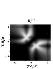
(b)

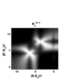
Figure 11: Topo graphs of long-time experimental quadratic negativities $N_{q}^{(2),\rm lt}$ depending on relative frequencies $(E-E_{b})/\Gamma$ and $(E^{\prime}-E_{b})/\Gamma$ and showing the correlations (a) inside one spectral region and (b) between two different spectral regions; $\Delta E/\Gamma=0.001$, values of the other parameters are written in the caption to Fig. 3.

Strong correlations are found among the frequencies $E$ and $E^{\prime}$ lying inside one spectral peak, but different sub-peaks [see Fig. 10(a)]. On the other hand, strong correlations occur also for the frequencies $E$ and $E^{\prime}$ localized inside the neighbor spectral peaks. Here, the correlations are observed inside the lower-frequency sub-peaks of two neighbor spectral peaks as well as inside the upper-frequency sub-peaks of the neighbor peaks [see Fig. 10(b)]. This example illustrates richness of the internal spectral structure of entangled stated in the investigated system.

VII Conclusions

The entanglement between two electrons in an auto-ionization atom and a neighbor two-level atom has been investigated. An expression for the negativity of a bipartite system composed of a qubit and a general system including both the discrete and continuum levels has been derived. The spectral density of quadratic negativity has been introduced to study the spectral features of entanglement. It has allowed to decompose the overall entanglement into the qubit-qubit entanglement of the constituting parts. Also the concept of experimental quadratic negativities has been introduced. It has been shown that the dipole-dipole interaction creates the entanglement between electrons until one of them is completely ionized. This puts restrictions to the strength of ionization paths in the auto-ionization atom. However, the balancing of two ionization paths in the auto-ionization atom results in a lower ionization speed that is in favor of the entanglement generation. Highly entangled states stable for long times are then reached. The entanglement is spectrally ’concentrated’ below the peaks of the long-time ionization spectra. Strong correlations have been found for pairs of frequencies localized inside one spectral peak as well as when two frequencies have been positioned below the neighbor peaks.

Appendix A Alternative derivation of the formula (43) for negativity $N$

We may conveniently decompose the functions $d_{0}(E)$ and $d_{1}(E)$ characterizing an ionized electron at atom $b$ in a suitable orthonormal basis formed by functions $f_{0}(E)$ and $f_{1}(E)$. In this basis, the problem of quantifying entanglement between the two-level system $a$ and the system $b$ with the continuum of states is reduced to the problem of quantifying the entanglement in a qubit-qubit system. The appropriate basis functions $f_{0}(E)$ and $f_{1}(E)$ can be constructed along the following recipe:

$$f_{0}(E) = \frac{d_{0}(E)}{\sqrt{b_{00}}},$$

$$f_{1}(E) = \frac{-b_{10}d_{0}(E)+b_{00}d_{1}(E)}{b_{00}b_{11}-|b_{01}|^{2}};$$ (62)

the coefficients $b_{jk}$ have been defined in Eq. (39). The inverse transformation to that written in Eq. (62) can be derived in the form:

$$d_{0}(E) = \alpha_{00}f_{0}(E),$$

$$d_{1}(E) = \alpha_{10}f_{0}(E)+\alpha_{11}f_{1}(E);$$ (63)

$\alpha_{00}=\sqrt{b_{00}}$, $\alpha_{10}=b_{10}/\sqrt{b_{00}}$, and $\alpha_{11}=(b_{00}b_{11}-|b_{10}|^{2})/b_{00}$.

Using new basis vectors $|0\rangle\rangle_{b}$ and $|1\rangle\rangle_{b}$ in the continuum of states at atom $b$,

$$|j\rangle\rangle_{b}=\int\,dEf_{j}(E)|E\rangle,\hskip 14.22636ptj=0,1,$$ (64)

the state vector $|\psi\rangle^{\rm lt}$ in Eq. (5) can be recast into the following long-time form:

$$|\psi\rangle^{lt} = \alpha_{00}|0\rangle_{a}|0\rangle\rangle_{b}+\alpha_{10}|1\rangle_{a}|0\rangle\rangle_{b}+\alpha_{11}|1\rangle_{a}|1\rangle\rangle_{b}.$$

The state vector $|\psi\rangle^{\rm lt}$ can be considered as a state of two qubits, $a$ and $b$. The partially transposed statistical operator $\varrho^{Ta}$, transposed with respect to the indices of atom $a$, can be written in the following matrix form:

$$\varrho^{Ta}=\left[\begin{array}[]{cccc}\alpha_{00}^{2}&0&\alpha_{00}\alpha_{10}&0\\ 0&0&\alpha_{00}\alpha_{11}&0\\ \alpha_{00}\alpha_{10}^{*}&\alpha_{00}\alpha_{11}&|\alpha_{10}|^{2}&\alpha_{10}\alpha_{11}\\ 0&0&\alpha_{10}^{*}\alpha_{11}&\alpha_{11}^{2}\end{array}\right].$$ (66)

The secular equation for the matrix $\varrho^{Ta}$ can be obtained in the form $(\lambda^{2}-{\cal D})(\lambda^{2}-p\lambda+{\cal D})=0$, where $p=\alpha_{00}^{2}+\alpha_{11}^{2}+|\alpha_{10}|^{2}$ and ${\cal D}$ has been defined in Eq. (41). The only negative solution of the secular equation, $\lambda=-\sqrt{\cal D}$, gives the formula for negativity $N$ given in Eq. (43).