Hypervelocity Planets and Transits Around Hypervelocity Stars

Abstract

The disruption of a binary star system by the massive black hole at the Galactic Centre, SgrA*, can lead to the capture of one star around SgrA* and the ejection of its companion as a hypervelocity star (HVS). We consider the possibility that these stars may have planets and study the dynamics of these planets. Using a direct $N$-body integration code, we simulated a large number of different binary orbits around SgrA*. For some orbital parameters, a planet is ejected at a high speed. In other instances, a HVS is ejected with one or more planets orbiting around it. In these cases, it may be possible to observe the planet as it transits the face of the star. A planet may also collide with its host star. In such cases the atmosphere of the star will be enriched with metals. In other cases, a planet is tidally disrupted by SgrA*, leading to a bright flare.

1 Introduction

Hypervelocity stars (HVSs) were first theorized in 1988 (Hills, 1988), and discovered observationally in 2005 (Brown et al., 2005). At least 16 HVSs have been identified in the Milky Way (Edelmann et al. 2005; Hirsch et al. 2005; Brown et al. 2006a; Brown et al. 2006b; Brown et al. 2007; Brown et al. 2009).There are a number of proposed mechanisms for the production of HVSs. The best studied and arguably most likely mechanism is the Hills’ scenario where the close interaction of a binary star system and massive black hole (MBH) can produce a HVS with sufficient velocity to escape the gravitational pull of the Milky Way (Hills 1988; Gould & Quillen 2003; Yu & Tremaine 2003; Ginsburg & Loeb 2006; Perets et al. 2007; Perets 2009a; Madigan et al. 2009, 2011). Other mechanisms include the interaction of stars with stellar black holes (O’Leary & Loeb, 2008), the inspiral of an intermediate mass black hole (Hansen & Milosavljević 2003; Yu & Tremaine 2003; Levin 2006; Sesana et al. 2009), and the disruption of a triple system (Lu et al. 2007; Sesana et al. 2009; Perets 2009b; Ginsburg & Perets 2011). We focus on the disruption of a tightly bound binary by a central black hole of inferred mass $\sim 4\times 10^{6}M_{\odot}$ (e.g. Schödel et al. 2003; Reid & Brunthaler 2004; Ghez et al. 2005; Ghez et al. 2008; Gillessen et al. 2009).

Simulations show that tight binaries disrupted by the MBH can result in the ejection of one component with velocities comparable to those of the observed HVSs (e.g. Ginsburg & Loeb 2006; Bromley et al. 2006), and perhaps significantly larger velocities as well (Sari et al., 2010). When a hypervelocity star is produced, the companion to the HVS is left in a highly eccentric orbit around SgrA* (Ginsburg & Loeb, 2006). Furthermore, a small fraction of binary systems may collide when disrupted, and if the collision velocity is small enough the system can coalesce (Ginsburg & Loeb, 2007; Antonini et al., 2011). For planets orbiting a star, tidal dissipation will eventually result in the infall of short-period planets into their host star (e.g. Rasio et al. 1996; Jackson et al. 2009); however the timescale is on the order of Gyrs, and planets with orbital periods of $\lesssim 1$ day are predicted to survive while the host star is on the main-sequence (Hansen, 2010). A number of Jupiter-mass planets have already been found with orbital periods $\lesssim 1$ day (e.g. Hebb et al. 2010; Hellier et al. 2011). Thus, it is only natural to consider the scenario where planets are orbiting such tightly bound binary systems which are subsequently disrupted by the MBH. Our goal is to examine the possible orbital dynamics and determine whether a HVS may host a planetary system.

In §2 we describe the codes and simulation parameters. In §3 we discuss the origin of hypervelocity planets (HVPs) and transits around HVSs, and in §4 we discuss some possible outcomes for the disruption of a binary system with planets. Our goal was not to cover the entire available phase space, but to determine whether some tight binaries with planets could produce transits or other observable effects.

2 Computational Method

In our study we have used the publically available N-body code written by Aarseth (1999) . We adopted a small value of $10^{-8}$ for the accuracy parameter $\eta$, which determines the integration step through the relation $dt=\sqrt{{\eta F}/(d^{2}F/dt^{2})}$ where $dt$ is the timestep and $F$ is the force. The softening parameter, eps2, which is used to create the softened point-mass potential, was set to zero. We treat the stars and planets as point particles and ignore tidal and general relativistic effects on their orbits, since these effects are small at the distance ($\gtrsim 10$AU) where the binary star system is tidally disrupted by the MBH. In total, we ran over 8000 simulations.

We set the mass of the MBH to $M=4\times 10^{6}M_{\odot}$, and the mass of each star to $m=3M_{\odot}$, which is comparable to the known masses of HVSs (Fuentes et al. 2006; Przybilla et al. 2008). Since the planet’s mass $\ll m_{\star}$ we treat all planets as test particles. All runs start with the centre of the binary system located 2000 AU ($=10^{-2}$pc) away from the MBH along the positive y-axis. This distance is larger than the binary size or the distance of closest approach necessary to obtain the relevant ejection velocity of HVSs, making the simulated orbits nearly parabolic. Our simulations include orbits in a single plane as well as simulations with the binary coming out of the orbital plane at $90^{\circ}$. For simplicity, the planetary orbital plane was kept the same as that of the binary. We used the same initial distance for all runs to make the comparison easier to interpret as we varied the distance of closest approach to the MBH or the relative positions of the stars and planets within the system.

We ran two primary sets of simulations. The first set consisted of a binary system with two planets. Each star had one planet initially at $a_{p}=0.02$ AU from its host star on a circular orbit (with eccentricity $e=0$). The second set consisted of a binary system with four planets. Initial conditions were similar to the previous data set, with the exception that the second planet was placed on a circular orbit with distance $a_{p}=0.03$ AU from the star. We varied the initial separation between the two stars from $a_{\star}=0.05$ to $0.5$ AU and precluded tighter binaries for which two stars develop a common envelope and coalesce. Similarly, much wider binaries may not produce HVSs (Hills 1991; Bromley et al. 2006; Ginsburg & Loeb 2006). However, in our simulations we assume planetary distances significantly shorter than $0.02$ AU would bring the planet into the star’s atmosphere and thus are precluded. Similarly, too large a distance could result in a dynamical instability whereby the planets are ejected from the system or collide with a star. In order to determine the effect of the planetary separation on the orbital dynamics, we ran additional simulations with a fixed binary semimajor axis $a_{\star}=0.2$ AU and varied the planetary separation in the range $a_{p}=0.02$–$0.06$ AU. Our simulations excluded planets around single stars since such systems will never produce HVSs.

A three-body encounter can lead to chaos, and the initial phase of the stellar orbit can greatly vary the outcome (Ginsburg & Loeb, 2006). Therefore, we sampled cases with initial phase values of $0$–$360^{o}$ at increments of $15^{o}$. We gave the binary system no radial velocity but a tangential velocity with an amplitude such that the effective impact parameter ($b$) is in the range of $5$–$35$ AU. The distribution of impact parameters is as follows: our simulations had $b=5,10,15,20$ AU with a likelihood of $\sim 20$% of all runs for each value, while the remainder at $b=25$ or $30$ AU had a $\sim 10\%$ likelihood each. We expect no HVSs to be produced at substantially larger impact parameters (Ginsburg & Loeb, 2006).

3 Origin of Hypervelocity Stars and Hypervelocity Planets

Given a binary system with stars of equal mass $m$ separated by a distance $a$ and a massive black hole (MBH) of mass $M\gg m$ at a distance $b$ from the binary, tidal disruption would occur if $b\la b_{\rm t}$ where

$$\frac{m}{a^{3}}\sim\frac{M}{{b^{3}_{\rm t}}}.$$ (1)

The distance of closest approach in the initial plunge of the binary towards the MBH can be obtained by angular momentum conservation from its initial transverse speed $v_{\perp}$ at its initial distance from the MBH, $d$,

$$v_{\perp}d=\left(\frac{GM}{b}\right)^{1/2}b.$$ (2)

The binary will be tidally disrupted if its initial transverse speed is lower than some critical value,

$$v_{\perp}\la v_{\perp,\rm crit}\equiv{(GMa)^{1/2}\over d}\left({M\over m}\right)^{1/6}=10^{2}{a_{-1}^{1/2}\over m_{0.5}^{1/6}d_{3.3}}~{}{\rm{km~{}s^{-1}}},$$ (3)

where $a_{-1}\equiv({a}/{0.1~{}{\rm AU}})$, $d_{3.3}=(d/2000~{}{\rm AU})$, $m_{0.5}\equiv(m/3M_{\odot})$, and we have adopted $M=4\times 10^{6}M_{\odot}$. For $v_{\perp}\la v_{\perp,\rm crit}$, one of the stars receives sufficient kinetic energy to become unbound, while the second star is kicked into a tighter orbit around the MBH. The ejection speed, $v_{\rm ej}$, of the unbound star can be obtained by considering the change in its kinetic energy $\sim v\delta v$ as it acquires a velocity shift of order the binary orbital speed $\delta v\sim\sqrt{Gm/a}$ during the disruption process of the binary at a distance $\sim b_{t}$ from the MBH when the binary centre-of-mass speed is $v\sim\sqrt{GM/b_{t}}$ (Hills, 1988; Yu & Tremaine, 2003). At later times, the binary stars separate and move independently relative to the MBH, each with its own orbital energy. For $v\la v_{\perp,\rm crit}$, we therefore expect

$$v_{\rm ej}\sim\left[\left({\frac{Gm}{a}}\right)^{1/2}\left({\frac{GM}{b_{\rm t}}}\right)^{1/2}\right]^{1/2}$$

$$=1.7\times 10^{3}m^{1/3}_{0.5}a^{-1/2}_{-1}~{}{\rm km~{}s^{-1}}.$$ (4)

A planet with mass $m_{p}\ll m_{\star}$ may also be ejected at even higher speeds. The mechanism that ejects HVPs involves the interaction of the MBH, the binary star system, and the planet, and does not admit a simple analytical estimate. Based on our simulations, the velocities of hypervelocity planets (HVPs) are on average $\sim 1.5$–$4$ times the velocity of a typical HVS (see Table 1). We found a few examples of HVPs with exceptionally high speeds, $v\sim 10^{4}$ km s^-1, however as observed in Figure 1, these are rare with a probability $<1$%. Although Figure 1 represents one specific parameter set, we do get comparable results for other runs.

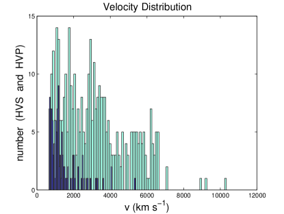
Figure 1: Velocity distribution of HVSs and HVPs. This sample comes from 1000 simulations. The initial binary separation for each system was $a_{\star}$ = 0.2 AU, and we let the planetary separation vary with uniform probability in the range $a_{p}=0.02$–$0.04$ AU. These runs are strictly for systems with two planets, however we get similar distributions for systems with four planets. The lowest HVP velocities are $\sim 700$ km s^-1, which corresponds with the lowest velocities for HVSs. The average HVP velocity is $\sim 3000$ km s^-1, and the average HVS velocity is $\sim 1500$ km s^-1 (see also Table 1). The HVPs are denoted in light blue, and the HVSs in the darker color. The overall shape of the distribution is similar in both cases, and in both cases there are outliers. Note that there are $\sim 3$ HVPs for each HVS.

$a_{\star}$ (AU)	$\bar{v}_{HVS}$ (km s-1)	$\bar{v}_{HVP}$ (km s-1)
0.05	2700	3800
0.10	2000	3100
0.20	1400	3500
0.30	1300	4100
0.40	1400	4100
0.50	1100	4400
0.05	-	-
0.10	-	-
0.20	1500	3300
0.30	1300	3900
0.40	1400	4200
0.50	1100	4200

Table 1: Average velocity of HVSs (second column) and HVPs (third column) for different values of $a_{\star}$. The top four rows show the values obtained from our simulations with two planets, and the bottom rows our results with four planets. For our simulations with four planets, the outer planets either collided with a star or were immediately ejected when $a_{\star}<0.2$ AU, hence no values are listed for 0.05 and 0.10 AU. All values are uncertain to within $\pm 50$ km s^-1

.

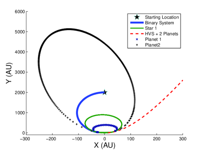
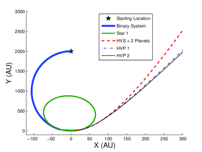
Figure 2: The two panels illustrate possible outcomes after a binary system with planets is disrupted by the MBH. The MBH is located at the origin, and the binary system starts at an initial distance of 2000 AU along the positive y-axis. In both cases the initial binary separation was $a_{\star}=0.2$ AU and the planetary separation $a_{p}=0.02$ AU for the innermost planets and $a_{p}=0.03$ AU for the outer planets. Left: After binary disruption a HVS is produced with two bound planets, as marked by the dashed line. The second star, marked by the solid line, stays in a highly eccentric orbit around the MBH. The second star’s planets are removed, and the first falls into a highly eccentric orbit close to the MBH, while the second is ejected into a much larger, but also highly eccentric orbit around the MBH. Right: After binary disruption a HVS is produced with two planets in orbit as marked by the dashed line. The second star, marked by the solid line, remains in a highly eccentric orbit around the MBH. The second star’s planets are ejected as HVPs.

4 The Fate of Planetary Systems

We analyze statistically the orbital properties of the binary star system after it is disrupted by the MBH. We ran simulations both planar and with the binary out of the orbital plane at $90^{\circ}$. In our simulations the initial planetary semimajor axis is constrained. Too small a separation would lead to a plunge of the planet into the host star’s atmosphere, and too large a separation would result in an unstable configuration in which the planet ultimately collides with a star or else is ejected from the system.

Figure 2 illustrates two possible outcomes. In both instances, HVSs with orbiting planets are produced (dashed line), while the companion star (solid line) orbits the MBH in a highly eccentric orbit. The companion star’s planets are themselves removed, and either stay bound to the MBH in different orbits or are ejected as HVPs. Table 2 shows various outcomes from our simulations including the fraction of HVPs, planets around HVSs, and free planets around the MBH.

$a_{\star}$ (AU)	HVSs	HVPs	HVSs + Planets	Bound Stars + Planets	Free Planets
0.05	0.40$\pm 0.03$	0.36$\pm 0.03$	0.05$\pm 0.01$	0.08$\pm 0.01$	0.80$\pm 0.03$
0.10	0.37$\pm 0.03$	0.36$\pm 0.03$	0.08$\pm 0.01$	0.35$\pm 0.03$	0.63$\pm 0.03$
0.20	0.20$\pm 0.02$	0.42$\pm 0.03$	0.05$\pm 0.01$	0.40$\pm 0.03$	0.58$\pm 0.02$
0.30	0.07$\pm 0.01$	0.39$\pm 0.03$	0.02$\pm 0.01$	0.35$\pm 0.03$	0.62$\pm 0.03$
0.40	0.03$\pm 0.01$	0.35$\pm 0.03$	0.01$\pm 0.01$	0.39$\pm 0.03$	0.62$\pm 0.03$
0.50	0.02$\pm 0.01$	0.43$\pm 0.03$	0.01$\pm 0.01$	0.42$\pm 0.03$	0.57$\pm 0.02$
0.05	-	-	-	-	-
0.10	-	-	-	-	-
0.20	0.19$\pm 0.02$	0.83$\pm 0.04$	0.11$\pm 0.02$	0.59$\pm 0.04$	0.64$\pm 0.02$
0.30	0.05$\pm 0.01$	0.70$\pm 0.04$	0.03$\pm 0.01$	0.59$\pm 0.04$	0.67$\pm 0.02$
0.40	0.02$\pm 0.01$	0.71$\pm 0.04$	0.01$\pm 0.01$	0.63$\pm 0.04$	0.65$\pm 0.02$
0.50	0.02$\pm 0.01$	0.78$\pm 0.04$	0.01$\pm 0.01$	0.76$\pm 0.04$	0.60$\pm 0.02$

Table 2: Probability for various outcomes in our ensemble of runs. The top rows show the results for simulations with two planets, and the bottom rows for our simulations with four planets. Note that for our simulations with four planets, the outer planets either collided with a star or were immediately ejected when $a_{\star}<0.2$ AU, hence no values are listed for 0.05 and 0.10 AU. The distance between each planet and host star is $a_{p}=0.02$ AU, and for simulations with four planets the second set of planets had $a_{p}=0.03$ AU. The first column is the initial distance between the two stars. The second column shows the fraction of HVSs produced, and as expected tighter binaries produce more HVSs. The third column shows the rate of HVP production. The fourth column shows the probability of producing HVSs with planets in orbit. This column is also represented graphically in the middle panel of Figure 3. The fifth column shows the fraction of stars that are bound to the MBH and have planets in orbit which may produce transits (see Section 4.4). The last column shows the fraction of free planets around the MBH. Probabilities in each row are independent of each other. Note that the sum of the probabilities for each row add to more than one due to the fact that we have two or four stars for each simulation. Therefore, as illustrated in Figure 2, there may be multiple outcomes for any given simulation. The quoted values include Poisson errors.

4.1 HVPs

Our simulations show that for tight binaries with semimajor axes in the range $a_{\star}=0.05$–$0.5$ AU and planets with semimajor axes $a_{p}=0.2$–$0.05$ AU, the probability of producing HVPs is high (see Table 2). For a binary with two planets, we find that the probability of producing a HVP is $\sim 30$–$40$%. For a binary with four planets, the probability rises to $\sim 70$–$80$%. However, since planets are extremely faint, it is impossible to detect HVPs directly with existing telescopes.

4.2 Transits Around HVSs

The probability of observing an eclipse as a planet orbits its host star is the transit probability ($P_{T}$) given by

$$P_{T}=\left(\frac{R_{\star}\pm R_{P}}{a}\right)\left(\frac{1+e\sin\omega}{1-e^{2}}\right),$$ (5)

where $R_{\star}$ is the star’s radius, $R_{P}$ the planet’s radius, $e$ is the eccentricity, and $\omega$ is the argument of periapse (see Murray & Correia 2010; Winn 2010). Note that the $+$ sign in equation (5) includes grazing eclipses, which are otherwise excluded. When $R_{\star}\gg R_{P}$ and $e=0$, we get

$$P_{T}\approx 0.015\left(\frac{R_{\star}}{3R_{\odot}}\right)\left(\frac{1{\rm AU}}{a}\right).$$ (6)

For massive ($m\geq 1M_{\odot}$) stars on the main-sequence, it is safe to assume $R_{\star}\gg R_{P}$ and thus the probability of a transit is independent of planetary radius. However, the fractional flux decrement is given by $(R_{p}/R_{\star})^{2}$. Therefore a larger planetary radius is important in order to be able to get proper photometry. We assume a Jupiter-sized planet, thus $(R_{p}/R_{\star})^{2}\sim 1$%. Our simulations produced planets orbiting HVSs with $\bar{e}$ = 0.6. Although an eccentricity will increase the probability of a transit, equation (5) is sensitive to high eccentricity and for a limiting case it is reasonable to use $e=0$. The timescale for eccentricity damping, whereby a planet’s eccentricity is circularized is not well understood, and depending on initial conditions one can get either short ($\sim 100$ Myr) or long ($\sim$ Gyr) circularization times (Naoz, 2012). Furthermore, $e=0$ is consistent with the observed eccentricities for most extrasolar planets with $a_{p}<0.1$ AU (e.g. Jackson et al. 2008; Hansen 2010; Matsumura et al. 2010).

Table 2 shows the probability of producing a HVS with orbiting planets. This probability is calculated as the fraction of all the runs we conducted in the restricted range of parameters for which HVSs are produced. We used a binary semimajor axis between $a_{\star}=0.05$–$0.5$ AU. Smaller $a_{\star}$ would lead to a common envelope and are precluded. Larger $a_{\star}$ are likely to either eject the planet from the system before producing a HVS, lead to a collision, or fail to produce a HVS altogether. The results for our simulations with two planets and four planets are qualitatively similar with some expected statistical variations, as illustrated in the middle panel of Figure 3. Our simulations also indicate that the planetary semimajor axis needs to be between $a_{p}=0.02$–$0.05$ AU in order for a planet to remain bound to a HVS. Smaller $a_{p}$ are precluded due to the fact that they would sink into the star’s atmosphere, and at larger $a_{p}$ the planets are tidally removed before the HVS is produced. For two-planet systems with $a_{\star}=0.2$ AU, we find that when $a_{p}=0.02$–$0.05$ AU the probability of producing a HVS with planets is constant. We get similar results for four planets, however the probability starts to rapidly decrease when $a_{p}=0.04$ AU. These results are illustrated in the right panel of Figure 3. In total, we find that the probability of producing a HVS with planets peaks at $\sim 10$%. Assuming a HVS has planets in orbit, the probability of observing a transit is given by equation (6). We plot these probabilities in Figure 4.

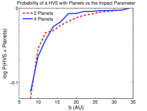
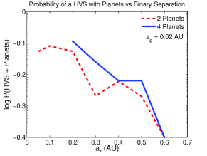
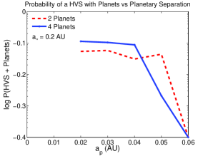
Figure 3: Probability of producing a HVS with orbiting planets versus various parameters. Left: Probability as a function of impact parameter, $b$, relative to SgrA*. This cumulative plot shows that an impact parameter between $10-20$ AU is optimal. The probabilities here are defined relative to all our HVS runs. Middle: Probability as a function of the initial distance between the two stars. In this scenario we exclude simulations with four planets when $a_{\star}<0.2$ AU, due to the fact that at such distances the two outermost planets were disrupted and either collided with a star or were ejected. The initial planetary separation is $a_{p}=0.02$ AU for all runs with two planets, and for our simulations with four planets the second set of planets had initial distance $a_{p}=0.03$ AU. Right: Probability as a function of initial planetary separation, $a_{p}$. We precluded orbits with $a_{p}<0.02$ AU, since such orbits would take the planet into the star’s atmosphere. The results for each figure are averaged for all orbits, those in a single plane and orbits out of the plane. The values of $a_{p}$ displayed along the $x$-axis correspond to the first set of planets. For simulations with four planets, the second set was placed $0.01$ AU from the first. Note that for the middle and right panels the impact parameter is not constrained.

Figure 4: Probability of observing a transit for a planet orbiting a HVS. Left: Probability of a transit (log $P_{T}$) vs the initial binary separation ($a_{\star}$). We exclude simulations with four planets when $a_{\star}<0.2$ AU, since the outermost planets are unstable at these parameters. Right: Probability of a transit (log $P_{T}$) vs the initial distance between the planet and host star ($a_{p}$). In this scenario $a_{\star}$ is fixed at 0.2 AU. In both instances, our results for two planets and four planets are qualitatively similar. The probability of observing a transit ranges from $0.35-0.90$.

4.3 Collisions

Assuming that a binary is disrupted at a random angle and ignoring gravitational focusing, the probability for a collision is

$$P\sim\frac{4R_{*}}{2\pi R_{\rm sep}},$$ (7)

where $R_{\star}$ is the radius of the star (assuming radii are approximately equal) and $R_{\rm sep}$ is the average separation of the stars. The stars will merge if the relative velocity of impact is less than the escape velocity from the surface of the star ($\sim 500~{}{\rm km~{}s}^{-1}$). A simple estimation for the impact velocity comes from conservation of energy,

$$E=\frac{1}{2}\frac{m_{1}m_{2}}{m_{1}+m_{2}}\dot{r}^{2}-\frac{Gm_{1}m_{2}}{r}=const,$$ (8)

which yields the relative impact velocity for two stars

$$v_{f}=\left[2G(m_{1}+m_{2})\left(\frac{1}{a_{min}}-\frac{1}{a}\right)\right]^{1/2}.$$ (9)

Similarly, for a planet around a star, we arrive at

$$v_{f}\sim\left[Gm_{\star}\left(\frac{2a-r}{ra}\right)\right]^{1/2}.$$ (10)

Equations (9) and (10) yield a velocity similar to the escape speed from the surface of the star $v\sim 500$ km ${\rm s}^{-1}$, however they do not take tidal forces nor gravitational focusing into account, therefore the actual impact velocities are expected to be slightly higher. For a Jupiter-like planet, a direct collision will release at minimun $10^{45}$ erg, and thus might be observable as a flare.

The rate of HVS production in the Milky Way is $\sim 10^{-5}{\rm~{}yr}^{-1}$ (Brown et al., 2006b), and the total collisional rate between stars is $\sim 10$ % (Ginsburg & Loeb, 2007). Based on our simulations, we find that the collisional probability for a system with two planets is $\sim 0.1$%, whereas for a system with four planets it is $\sim 1$%. For systems with four planets, the collisions are almost entirely due to the two outer planets.

Should a planet collide with its host star, the planet will be destroyed and add high-metallicity material to the star’s surface. The metallicity of stars with planetary systems has been shown to be greater than expected by a factor of $\sim 2$ (e.g. Santos et al. 2003; Vauclair 2004). Such high metallicity may be due to tidal interactions that have caused exoplanets to fall into their host stars (Levrard et al., 2009; Jackson et al., 2009). Although the mechanism by which a star may lose its high-metallicity material is not well understood (Sasselov, 2012), Garaud (2011) has shown that the relative metallicity enhancement on the surface due to the infall of exoplanets, survives a much shorter period for higher-mass stars. A star of $1.5M_{\odot}$ would lose $\sim 90$% of its enhanced metallicity in merely 6 Myr. Thus, a HVS (typically found at large distances from their origin at the Galactic Centre) may have lost nearly all its enhanced metallicity relatively early. Furthermore, metal-rich HVSs have not been detected (Kollmeier et al., 2011). We suggest that if current or future HVSs are found with enhanced metallicity, it may be due to a relatively recent planetary collision.

4.4 Bound and Free Planets Around SgrA*

When a binary system is tidally disrupted by the MBH, a HVS may be produced while the companion star remains in a highly eccentric orbit around the MBH. If the disruption fails to produce a HVS, both stars will orbit the MBH. In either case, our simulations show a substantial probability for a planet to remain bound to a star that is in orbit around SgrA* (see Table 2). It is unclear whether in the long run such planets will be dynamically stable or eventually fall into their host stars. However, it is certainly possible that some of the stars near SgrA* host planetary systems. Should a star near the Galactic Center have a planet transit the surface, the change in magnitude will be $\delta m\sim 0.01$. Near-infrared photometry can get close to 0.01 mag precision, however extinction and the crowding of stars make such observations difficult (e.g. Schödel et al. 2010).

The probability for at least one planet to fall into a highly eccentric orbit around SgrA* is on average $>60$% for all our runs. If such a planet passes within the tidal radius of the MBH

$$R_{T}\sim R_{p}\left(\frac{M_{MBH}}{m_{p}}\right)^{1/3},$$ (11)

(where $R_{p}$ and $m_{p}$ are respectively the radius and mass of the planet), the tidal force will disrupt the planet. A star will similarly be disrupted if it passes too close to its tidal radius, and might produce an optical flare of $\sim 10^{43}$ erg s^-1 (Strubbe & Quataert, 2009). For a planet disrupted by the MBH, the accretion rate $\dot{M}$ mass would be lower, leading to a luminosity

$$L=\epsilon\dot{M}c^{2},$$ (12)

where $\epsilon$ is the radiative efficiency. Zubovas et al. (2011) suggest that asteroids disrupted by SgrA* may be responsible for flares with $L\sim 10^{34}-10^{39}$ erg s^-1. Furthermore, they note that a brighter flare ($L\sim 10^{41}$ erg s^-1) that is inferred to have occurred $\sim 300$ years ago may be due to the tidal disruption of a planet. Figure 5 shows the probability for a planet in orbit around the MBH to be tidally disrupted. The probability for a system with two planets is shown by the dashed line, and four planets by the solid line.

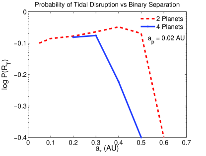
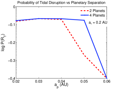
Figure 5: Probability for a planet freed during the production of a HVS from a binary star system, to be tidally disrupted by the MBH. Left: Probability as a function of the binary separation. We exclude simulations with four planets when $a_{\star}<0.2$ AU due to instability. Right: Probability as a function of planetary separation. $a_{p}=0.02$ AU was the minimum semimajor axis length. For $a_{p}=0.06$ AU the planets either crashed into a star or were removed, hence the probability is $\sim 0$. The origin of the break between the simulations with two planets (dashed line) and four planets (solid line) is due primarily to the fact that for four planets, the outer planets are easily disrupted with increasing $a_{\star}$, and are ejected or crash into a star before being tidally disrupted by the MBH. For increasing $a_{p}$, both two planet and four planet simulations have similar stability, however there are more planets in the latter case and thus the probability does not drop as quickly.

5 Conclusions

Our simulations show that in order to produce a HVS with planets in orbit, the initial binary separation needs to be in the range $a_{\star}=0.05$–$0.5$ AU, and the planetary separation in the range $a_{p}=0.02$–$0.05$ AU (e.g. “hot Jupiters”). For such parameters there is up to a $\sim 10$% probability that a HVS is produced with orbiting planets (see Table 2). In such scenarios there is a high probability that at least one planet transits the star (see Figure 4). For hot Jupiters, the fractional flux decrement in the light curve, $(R_{p}/R_{\star})^{2}\sim 1$%, would typically last for hours. Assuming no systematic errors, a powerful enough telescope can get milli-magnitude photometry (corresponding to fractional flux sensitivity of 0.1%) and hence determine whether or not a HVS has any transiting planets. Our examples of planets around HVSs have orbital periods in the range $0.3$ to $19$ days, requiring observing programs of this duration. The Hills’ mechanism that produces such HVSs also produces HVPs. Unfortunately, it is extremely difficult to detect a free HVP. Our simulations indicate that HVPs may achieve speeds $\sim 10^{4}$ km s^-1 in rare circumstances.

When a binary system with our given parameters is disrupted, it is possible that a planet will collide with its host star. In such instances the surface may be enriched with metals. Such an enrichment is not believed to last more than a few Myr for massive stars (Garaud, 2011). The age of HVSs exceed the time necessary for the excess metallicity in the star’s atmosphere to be erased. If observations show that a HVS has an unusually metal-rich atmosphere, this may indicate that a planet has relatively recently fallen into the star’s atmosphere.

Planets that are not ejected as HVPs and are not orbiting any HVSs, may still be detectable as transits around stars orbiting SgrA*. Assuming a Jupiter-like planet, the change in magnitude will be $\delta m\sim 0.01$. There is also a high probability that free-floating planets will be produced. It may not be possible to ascertain whether a free-floating planet was originally bound to a binary system that was disrupted. However, our simulations show that free-floating planets from disrupted systems should be in highly eccentric orbits around the MBH with an eccentricity $\sim 0.96$ or greater, similar to former companions to HVSs (Ginsburg & Loeb, 2006). Furthermore, it is also possible for a planet or star to be tidally disrupted by the MBH, producing a substantial flare from SgrA*. The luminosity and duration of the flare would indicate whether it was a planet ($L\sim 10^{40}$–$10^{41}$ erg s^-1) or star ($L\sim 10^{43}$ erg s^-1) that fed the MBH (Strubbe & Quataert 2009; Zubovas et al. 2011).

The detection of even one planet around a HVS can shed light on planetary formation and evolution within the central arcsecond of SgrA*. In particular, it would support the notion that young stars near the MBH have close-in planets. It has been suggested that planets and even asteroids may form in protoplanetary discs around stars orbiting a MBH (Nayakshin et al., 2012). Recently, a gas cloud was discovered plunging towards SgrA* (Gillessen et al., 2012). While it was suggested that this cloud originated from stellar winds or from a planetary nebula (Burkert et al., 2012), another theory is that it originated from a proto-planetary disk around a low-mass star, which implies that planets may form in the Galactic Centre (Murray-Clay & Loeb, 2012). The detection of a planet transiting a HVS would lend considerable support to this interpretation. If most stars in the Galactic centre form with planetary systems, then our simulations indicate that there should be planets in highly eccentric orbits around SgrA*.

References

- Aarseth (1999) Aarseth S. J., 1999, PASP, 111, 1333
- Antonini et al. (2011) Antonini F., Lombardi J., Merritt D., 2011, ApJ, 731, 128
- Bromley et al. (2006) Bromley B., Kenyon S., Geller M., Barcikowski E., Brown W., Kurtz M., 2006, ApJ, 653, 1194
- Brown et al. (2009) Brown W., Geller M., Kenyon S., 2009, ApJ, 690, 1639
- Brown et al. (2005) Brown W., Geller M., Kenyon S., Kurtz M., 2005, ApJL, 622, L33
- Brown et al. (2006a) Brown W., Geller M., Kenyon S., Kurtz M., 2006a, ApJL, 640, L35
- Brown et al. (2006b) Brown W., Geller M., Kenyon S., Kurtz M., 2006b, ApJ, 647, 303
- Brown et al. (2007) Brown W., Geller M., Kenyon S., Kurtz M., 2007, ApJ, 671, 1708
- Burkert et al. (2012) Burkert A., Schartmann M., Alig C., Gillessen S., Genzel R., Fritz T., Eisenhauer F., 2012, arXiv:1201.1414v1
- Edelmann et al. (2005) Edelmann H., Napiwotzki R., Heber H., 2005, ApJL, 634, L181
- Fuentes et al. (2006) Fuentes C., Stanek K., Gaudi B., McLeod B., Bogdanov S., Hartman J., Hickox R., Holman M., 2006, ApJL, 636, 37
- Garaud (2011) Garaud P., 2011, ApJL, 728, L30
- Ghez et al. (2005) Ghez A., Salim S., Hornstein S., Tanner A., Lu J., Morris M., Becklin E., Duchêne G., 2005, ApJ, 620, 744
- Ghez et al. (2008) Ghez A., Salim S., Weinberg N., Lu J., Do T., Dunn J., Matthews K., Morris M. R., Yelda S., Becklin E., Kremenek T., Milosavljevic M., Naiman J., 2008, ApJ, 689, 1044
- Gillessen et al. (2009) Gillessen S., Eisenhauer F., Fritz T., Bartko H., Dodds-Eden K., Pfuhl O., Ott T., Genzel R., 2009, ApJL, 707, L114
- Gillessen et al. (2012) Gillessen S., Genzel R., Fritz T., Quataert E., Alig C., Burkert A., Cuadra J., Eisenhauer F., Pfuhl O., Dodds-Eden K., Gammie C., Ott T., 2012, Nature, 481, 51
- Ginsburg & Loeb (2006) Ginsburg I., Loeb A., 2006, MNRAS, 368, 221
- Ginsburg & Loeb (2007) Ginsburg I., Loeb A., 2007, MNRAS, 376, 492
- Ginsburg & Perets (2011) Ginsburg I., Perets H., 2011, arXiv:1109.2284v1
- Gould & Quillen (2003) Gould A., Quillen A., 2003, ApJ, 592, 935
- Hansen (2010) Hansen B., 2010, ApJ, 723, 285
- Hansen & Milosavljević (2003) Hansen B., Milosavljević M., 2003, ApJL, 593, L77
- Hebb et al. (2010) Hebb L., Collier-Cameron A., Triaud A., et al. 2010, ApJ, 723, 285
- Hellier et al. (2011) Hellier C., Anderson D., Cameron A., Gillon M., Jehin E., Lendl M., Maxted P., Pepe F., Pollacco D., Queloz D., Ségransan D., Smalley B., Smith A., Southworth J., Triaud A., Udry S., West R., 2011, A&A, 535, L7
- Hills (1988) Hills J., 1988, Nature, 331, 687
- Hills (1991) Hills J., 1991, AJ, 102, 704
- Hirsch et al. (2005) Hirsch H., Heber U., O’Toole J., Bresolin F., 2005, A&A, 444, L61
- Jackson et al. (2009) Jackson B., Barnes R., Greenberg R., 2009, ApJ, 698, 1357
- Jackson et al. (2008) Jackson B., Greenberg R., Barnes R., 2008, ApJ, 678, 1396
- Kollmeier et al. (2011) Kollmeier J., Gould A., Rockosi C., Beers T., Knapp G., Johnson J., Morrison H., Harding P., Lee Y., Weaver B., 2011, ApJ, 723, 812
- Levin (2006) Levin Y., 2006, ApJ, 653, 1203
- Levrard et al. (2009) Levrard B., Winisdoerffer C., Chabrier G., 2009, ApJ, 692, L9
- Lu et al. (2007) Lu Y., Yu Q., Lin D., 2007, ApJL, 666, L89
- Madigan et al. (2011) Madigan A.-M., Hopman C., Levin Y., 2011, ApJ, 738, 99
- Madigan et al. (2009) Madigan A.-M., Levin Y., Hopman C., 2009, ApJL, 697, L44
- Matsumura et al. (2010) Matsumura S., Stanton J., Rasio F., 2010, ApJ, 725, 1995
- Murray & Correia (2010) Murray C., Correia A., 2010, Exoplanets. Arizona University Press, p. 15
- Murray-Clay & Loeb (2012) Murray-Clay R., Loeb A., 2012, arXiv:1112.4822v1
- Naoz (2012) Naoz S., 2012, private communication
- Nayakshin et al. (2012) Nayakshin S., Szonov S., Sunyaev R., 2012, MNRAS, 419, 1238
- O’Leary & Loeb (2008) O’Leary R., Loeb A., 2008, MNRAS, 383, 86
- Perets (2009a) Perets H., 2009a, ApJ, 690, 795
- Perets (2009b) Perets H., 2009b, ApJ, 698, 1330
- Perets et al. (2007) Perets H. B., Hopman C., Alexander T., 2007, ApJ, 656, 709
- Przybilla et al. (2008) Przybilla N., Nieva M., Tillich A., Heber U., Butler K., Brown W., 2008, A&A, 488, L51
- Rasio et al. (1996) Rasio F., Tout C., Lubow S., Livio M., 1996, ApJ, 470, 1187
- Reid & Brunthaler (2004) Reid M., Brunthaler A., 2004, ApJ, 616, 872
- Santos et al. (2003) Santos N., G. I., Mayor M., Rebolo R., Udry S., 2003, A&A, 398, 363
- Sari et al. (2010) Sari R., Kobayashi S., Rossi E., 2010, ApJ, 708, 605
- Sasselov (2012) Sasselov D., 2012, private communication
- Schödel et al. (2010) Schödel R., Najarro F., Muzic K., Eckart A., 2010, A&A, 511, A18
- Schödel et al. (2003) Schödel R., Ott T., Genzel R., Eckart A., Mouawad N., Alexander T., 2003, ApJ, 596, 1015
- Sesana et al. (2009) Sesana A., Madau P., Haardt F., 2009, MNRAS, 392, L31
- Strubbe & Quataert (2009) Strubbe L., Quataert E., 2009, MNRAS, 400, 2070
- Vauclair (2004) Vauclair S., 2004, ApJ, 605, 874
- Winn (2010) Winn J., 2010, Exoplanets. Arizona University Press, p. 55
- Yu & Tremaine (2003) Yu Q., Tremaine S., 2003, ApJ, 599, 1129
- Zubovas et al. (2011) Zubovas K., Nayakshin S., Markoff S., 2011, arXiv:1110.6872v1