Reconstruction of the wavefunctions of coupled nanoscopic emitters using a coherent optical technique

Abstract

We show how coherent, spatially resolved spectroscopy can disentangle complex hybrid wave functions into wave functions of the individual emitters. This way, detailed information on the coupling of the individual emitters, not available in far-field spectroscopy, can be revealed. Here we propose a quantum state tomography protocol that relies on the ability to selectively excite each emitter individually by spatially localized pulses. Simulations of coupled semiconductor GaAs/InAs quantum dots using light fields available in current nanoplasmonics show, that undesired resonances can be removed from measured spectra. The method can be applied on a broad range of coupled emitters to study the internal coupling, including pigments in photosynthesis and artificial light harvesting.

I Introduction

The formation of collective optical resonances from Coulomb-coupled optical emitters is a very general phenomenon, including examples from chromophores in biological light harvesting complexesEngel et al. (2007); Christensson et al. (2010); Wit (2011); Schoth et al. (2012), semiconductor quantum dots Guenther et al. (2002); Lovett et al. (2003), metal nanoparticles and composite systems, such as plasmon lasers Bergman and Stockman (2003).

For all these structures, dipole-dipole coupling occurs on a nanometer scale and the states of the individual emitters hybridize to form new collective, so called excitonic states, delocalized over the whole structure. Far field excitation, governed by the wavelength resolution limit $\lambda/2$, can only probe delocalized exciton states of a nanostructure. Related far-field experiments such as absorption, pump probe and four wave mixing are unable to disentangle the individual contributions of the coupled emitters from the collective optical response, because the exciting fields are spatially constant on the scale of the entire structure and cannot discriminate different emitters. In contrast, spatially local spectroscopy such as near field spectroscopy can, in principle, address the individual emitters.

In this paper, we propose a new class of measurements that combine coherent nonlinear spectroscopy with near field optics to reconstruct the contributions of single emitters to the delocalized wave function in a spatially extended nanostructure. As an example, we demonstrate, how a coherent double-quantum-coherence optical technique Abramavicius et al. (2009) may be combined with spatially localized fields to reconstruct the exciton wave functions of three dipole coupled self-organized GaAs/InAs quantum dots. This constitutes a particular quantum state tomography. The presented procedure is independent of the technique for localizing the fields at individual emitters. Several localization methods are known and are already applied to a broad range of nanoemitting structures, e.g. using (metalized) near field fiber tips von Freymann et al. (1998); Guenther et al. (1999, 2002), metal tips Pettinger et al. (2004); Weber-Bargioni et al. (2011), nano antennas Zhang et al. (2009); Kinkhabwala et al. (2009); Schuller et al. (2010); Curto et al. (2010); Novotny (2011) and metal structures combined with pulse shaped fields Stockman et al. (2002); Aeschlimann et al. (2007).

Quantum state tomography is a development aimed at the direct reconstruction of wave functions or more generally the density matrix, first proposed by Fano Fano (1957). The importance of quantum state tomography results from the fact, that the reconstruction and knowledge of the wave function opens the possibility to calculate new observables not related to optics at all. Examples include magnetic moments and transport properties. So far, wave functions are seldom directly accessible by experiments Gerhardt et al. (2010). Recent advances include imaging of single orbitals using soft-x-ray pulses Kapteyn et al. (2007); Corkum and Krausz (2007) and the reconstruction of states Yuen-Zhou and Aspuru-Guzik (2011); Lobino et al. (2008). Applications so far range from Spin 1/2 particles Band and Park (1979), photon states using the Wigner function Vogel and Risken (1989); Smithey et al. (1993), vibrational states Dunn et al. (1995) to Josephson junctions Steffen et al. (2006). In contrast to earlier approaches, the quantum state tomography developed in this paper combines optical fields, highly localized in time and space with coherent 2D spectroscopy, using a sequence of light pulses with controlled envelopes and phases Abramavicius et al. (2009); Li et al. (2006); Aeschlimann et al. (2011).

II Excitons in coupled nanostructures

As a typical example for coupled nanostructures with delocalized wave functions, we study three coupled self-organized semiconductor quantum dots Lovett et al. (2003); Danckwerts et al. (2006); Dachner et al. (2010), cp. Fig. 1a). The quantum dot distance is assumed to be sufficiently large to have no electronic wave function overlap between the quantum dots. In this case we study interdot coupling in the form of dipole-dipole (or Förster) coupling known from selforganized GaAs/InAs quantum dots: Parameters like dot size, dot distances, coupling constants, and energy shifts are well known from theory Richter et al. (2006) and experiment Unold et al. (2005). Each quantum dot is represented as a two level system. This is a valid assumption for quantum dots provided (i) quantum dots have no spin-orbit splitting and a big enough biexcitonic shift, (ii) are negatively charged or (iii) have spin-orbit coupling bigger than the inter quantum dot couplings Jacak et al. (1998); Borri et al. (2001). For selforganized quantum dots with sizes of $20\mathrm{nm}$ and interdot distances around $40\mathrm{nm}$, the dipole coupling is about several $\mu\mathrm{eV}$ with a Lorentzian zero phonon line (ZPL) width of $\gamma=1\mu\mathrm{eV}$ at low temperatures (e.g. $T=4K$) Borri et al. (2001); Stock et al. (2011). We neglected the influence of the phonon side bands, since their amplitude in the spectra is one to two orders smaller than the amplitude of the zero phonon line resonance at low temperatures Borri et al. (2001); Stock et al. (2011).

Three coupled quantum dots exhibit joint states: a ground state $g$, three single-exciton states $e_{1}$, $e_{2}$ and $e_{3}$ and three two-exciton states $f_{1}$, $f_{2}$ and $f_{3}$, cf. Fig. 1b). The system has one triexciton state, but these states are of no relevance in a third order optical experiment, considered here. The ground state of the uncoupled quantum dots is not changed by the induced dipole-dipole coupling. The delocalized single-exciton states $|e\rangle$ resulting from the dipole-dipole interaction are composed of local, uncoupled quantum dot states $|i\rangle$ (quantum dot $i$ in excited state): $|e\rangle=\sum_{i}c^{e}_{i}|i\rangle$. $|e\rangle$ is an energy eigenstate of the coupled quantum dot system, $c^{e}_{i}$ the expansion coefficients. Similarly, two-exciton states $|f\rangle$ are composed of states with two local excitations at quantum dot i and j: $|f\rangle=\sum_{i<j}c^{f}_{ij}|ij\rangle$. In general, excited states of $N$ coupled two level system emitters form a ground state $g$, $N$ delocalized single-exciton states $e$ and $N(N-1)/2$ delocalized two exciton states $f$. For our three dot case, we choose couplings between two quantum dots slightly stronger than to the third quantum dot (parameters given in Table 1). Here, $H_{0}$ includes along the diagonal the transition frequency local emitters modified by single and two exciton shifts, respectively. The offdiagonal elements describe interactions describing excitation transfer caused by e.g. dipole-dipole interactions.

a) $\langle i|H_{0}|j\rangle$ $1$ $2$ $3$ $1$ $2.0$ $1.0$ $0.2$ $2$ $1.0$ $0.2$ $0.1$ $3$ $0.2$ $0.1$ $-2.5$
b) $\langle ij|H_{0}|kl\rangle$ $1,2$ $1,3$ $2,3$ $1,2$ $\langle 1|H_{0}|1\rangle+\langle 2|H_{0}|2\rangle+V_{t1}$ $\langle 3|H_{0}|2\rangle$ $\langle 3|H_{0}|1\rangle$ $1,3$ $\langle 2|H_{0}|3\rangle$ $\langle 1|H_{0}|1\rangle+\langle 3|H_{0}|3\rangle+V_{t2}$ $\langle 2|H_{0}|1\rangle$ $2,3$ $\langle 1|H_{0}|3\rangle$ $\langle 1|H_{0}|2\rangle$ $\langle 1|H_{0}|1\rangle+\langle 3|H_{0}|3\rangle+V_{t3}$

Table 1: Hamiltonoperator in matrix form. a) The single exciton block and b) the two exciton states block. All values are given in $\mu eV$. The diagonal elements of the matrices are given as detuning to a mean gap frequency, a) $\omega_{gap}$ for the single excitons, b) $2\omega_{gap}$ for the two excitons, with $\omega_{gap}=1.053\mathrm{eV}$ and the two exciton shifts $V_{t1}=0.1\mu eV$, $V_{t2}=-2.5\mu eV$ and $V_{t3}=-1.5\mu eV$.

First, to characterize the system within far field spectroscopy, we calculate the linear absorption spectrum:

$$\alpha(\omega)\propto\sum_{e}\frac{|\mu_{eg}|^{2}}{(\omega-\omega_{eg})^{2}+\gamma^{2}}.$$ (1)

Here, $\mu_{eg}$ is the dipole moment for ground state to single-exciton transition, $\omega_{eg}$ is the transition frequency and $\gamma$ the dephasing constant.

The absorption spectrum of the coupled quantum dot structure is plotted in Fig. 2(solid). The single-exciton states $e_{1}$, $e_{2}$, $e_{3}$ overlap spectrally such that only $e_{1}$ and $e_{2}$ are well resolved, $e_{3}$ contributes only with a spectral shoulder. Comparing coupled and uncoupled(dashed) spectra, one recognizes, that the oscillator strength is originally evenly distributed but strongly modified, since the dipole-dipole coupling forms excitons delocalized over the entire structure.

III Ingredients for reconstructing delocalized states

Our main goal is to gain information on the built up of the delocalized wavefunctions of the excitonic states, i.e. on the expansion coefficients $c^{e}_{i}$, for a given single-exciton state $|e\rangle$. For this purpose, we use coherent, spatially local spectroscopy, composed of three ingredients:
(i) local nanoscale excitation provided by metallic nanoantennas and refined pulse shaping techniques Aeschlimann et al. (2007); Reichelt and Meier (2009) to optically address individual quantum dots, (Section III.1)
(ii) phase cycling of the optical response Meyer and Engel (2000); Tian et al. (2003); Brinks et al. (2010), to disentangle the total nonlinear response into desired quantum paths, (Section III.2)
(iii) a postprocessing procedure to calculate the coefficients $c^{e}_{i}$ (Section IV).

In general, (ii) and (iii) can be applied to any quantum system representable by spatial separated coupled emitters, if any localization technique (i) is available.

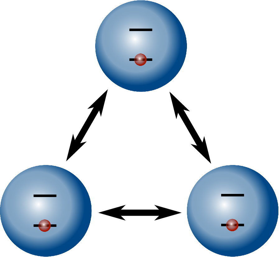
a) b)

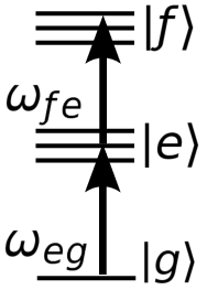
Figure 1: a) Three dipole-dipole coupled self-organized InAs quantum dots, b) Exciton level scheme of the three coupled quantum dots.

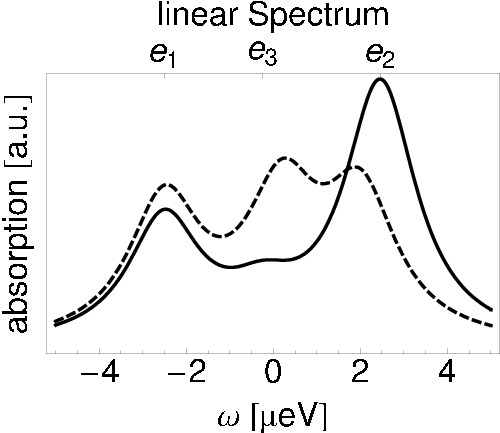
Figure 2: Absorption spectrum coupled (solid) and uncoupled (dashed) quantum dots. The detection frequency $\omega$ is given as detuning relative to frequency $\omega_{gap}=1.053\mathrm{eV}$ (transition frequency of uncoupled quantum dot 3).

III.1 Localized excitation

A main ingredient of our scheme is the local excitation of individual quantum dots. In our specific example, we achieve local excitation of the individual quantum dots by a plasmonic antenna structure of triangular symmetry on a subwavelength scale, cp. Fig. 3a). These metal structures can be realized by e-beam lithography. Solving Maxwell’s equations for this geometry shows that plasmonic effects and an optimization procedure of the applied pulses allows to selectively excite single quantum dots Brixner et al. (2005); Pomplun et al. (2007):

For optimizing the pulse envelope of a single pulse $\mathbf{E}(t,\mathbf{r})$ towards a field localization at only one quantum dot, we use time-harmonic solutions $\mathbf{E}_{\nu}(\omega,\mathbf{r})$, represented by incident plane waves of polarization directions $\mathrm{p},\mathrm{s}$ and incoming direction (indexed as $\nu$)Pomplun et al. (2007):

$$\mathbf{E}(t,\mathbf{r})=\frac{1}{\sqrt{2\pi}}\int_{-\infty}^{\infty}d\omega\sum_{\nu}g_{\nu}(\omega)\mathbf{E}_{\nu}(\omega,\mathbf{r})e^{-\imath\omega t}.$$ (2)

Pulse shaping is introduced by the weighting function:

$$g_{\nu}(\omega) = \sum_{n}f^{\nu}(\vartheta_{n})\frac{A_{n}}{\sqrt{2\pi}}e^{-(\eta_{n}-\omega)^{2}{\sigma_{n}}^{2}/{2}+\imath\omega\tau_{n}+\imath\beta_{n}},$$ (3)

which represents a composition of Gaussian pulses with amplitudes $A$, center times $\tau$, frequencies $\eta$, widths $\sigma$, phases $\beta$, and polarization angle $\vartheta$ for each pulse $n$ projected to polarization direction $\nu$ ($f^{\mathrm{p}}=\cos,f^{\mathrm{s}}=\sin$). $g_{\nu}(\omega)$ has to be determined by optimization. To increase the number of optimization parameters, we combine the three incoming pulses from three directions, using $120\textdegree$ symmetry of the sample. For this paper, details of the optimization procedure are of no relevance but can be found in Ref. Brixner et al., 2005; Reichelt and Meier, 2009. Later on, the absolutes value of $E(t)$ in the quantum dots centers is the input for the calculation of the localized spectra.

In Fig. 3b), the spatial field distribution for the optimized total field around the quantum dot transition frequency is shown. It can be recognized, that a chosen, single quantum dot is excited stronger than the other quantum dots. We observe field enhancements between different quantum dot sites of a factor of eight or larger. Note, that the optimized fields in frequency domain show that polarization and propagation phase effects cause localization and not a frequency based selection of different quantum dots.

Note, that the presented localization scheme using excitation pads is just an example. For application of the protocol to other systems Guenther et al. (2002); von Freymann et al. (1998); Guenther et al. (1999); Pettinger et al. (2004); Weber-Bargioni et al. (2011); Zhang et al. (2009); Kinkhabwala et al. (2009); Schuller et al. (2010); Curto et al. (2010); Novotny (2011); Stockman et al. (2002); Aeschlimann et al. (2007), other spatial localization schemes might be used.

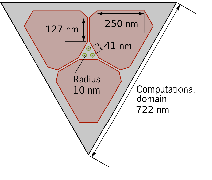
a) b)

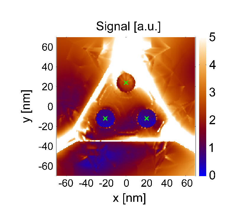
Figure 3: a) Schematic geometry: Three selforganized GaAs/InAs quantum dots (diameter $20\mathrm{nm}$, inter dot distances $40\mathrm{nm}$) and three $12\,\mathrm{nm}$ thick silver layer structures, arranged with 120° rotational symmetry on a semi infinite GaAs-layer. b) Optimized localized electric field $|E|$ at the maximum peak for a single pulse composed from shaped pulses from three different directions. Note: the white color is $5$ arbitary units or higher. The magnitude (extracted at X) of the optimized electric field $|E(\mathbf{r},\omega_{gap})|$ for $\omega_{gap}$ at dots 2 and 3 is $12\%$ or $7.5\%$ compared to dot 1. The field intensity is scalable while third order perturbation theory is valid for the double quantum coherence spectrum.

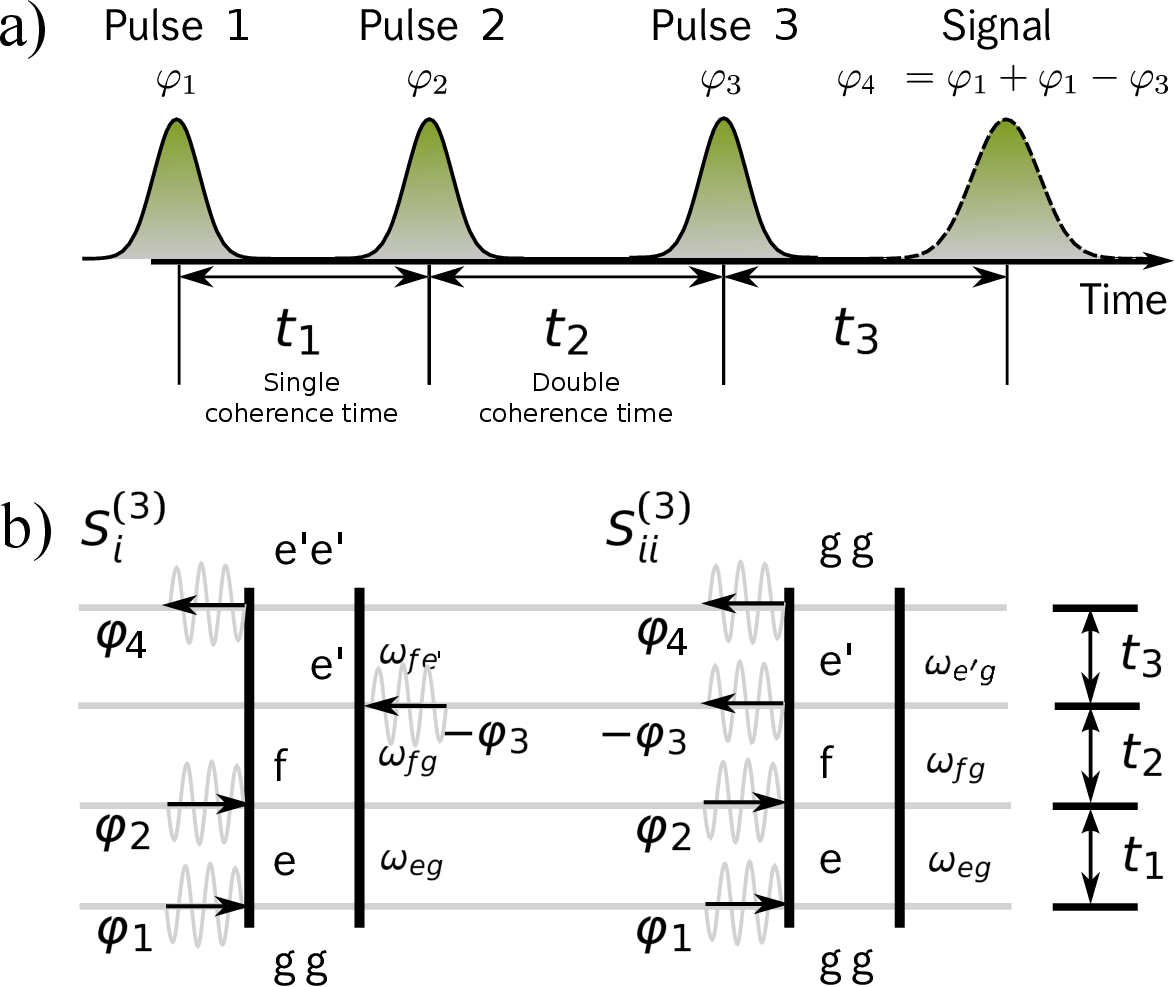
Figure 4: a) Pulse sequence for the double quantum coherence experiment. b) The two density matrix pathways $S_{i}$ and $S_{ii}$ ( Eq. 20). See text for more details.

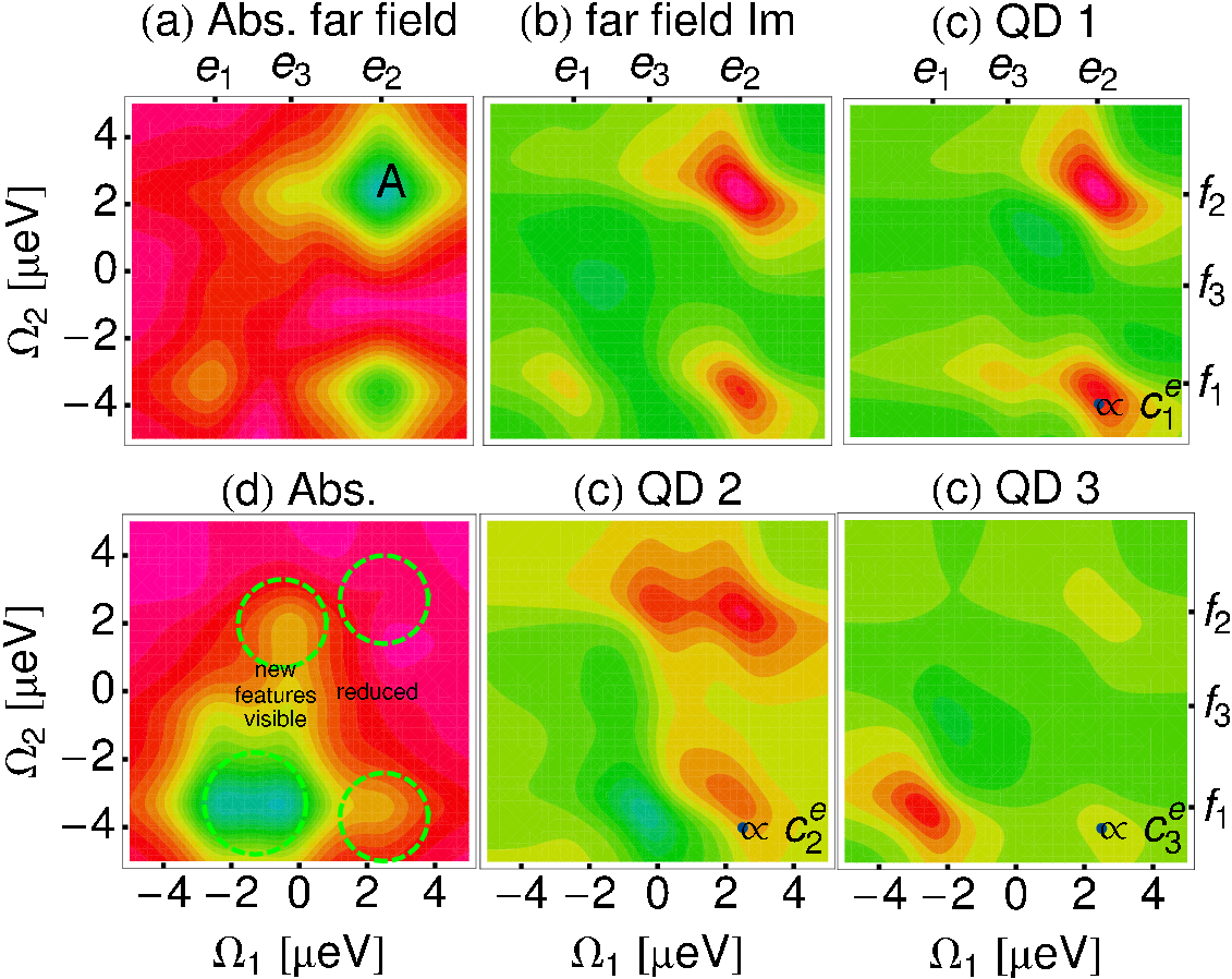
Figure 5: DQS for $t_{3}=200\mathrm{ps}$ a) absolute value b) imaginary part, $\Omega_{1}$ ($\Omega_{2}$) given as detuning around the single (double) gap frequency $\omega_{gap}$. c) Imaginary part of localized double quantum coherence spectrum, where the first pulse is localized at quantum dot 1, 2 and 3 as indicated d) Filtered standard double quantum coherence spectrum ($e_{2}$ removed).

III.2 Phase cycling detection of coherent signals

As explained in Sec. III.1, a sequence of three spatially optimized pulse envelopes $E^{i}$ with phases $\varphi_{i}$ and laser frequency $\omega_{l}$ is used Yang and Mukamel (2008); Abramavicius et al. (2009):

$$E(\mathbf{r},t) = E^{1}(\mathbf{r},t-t_{3}-t_{2}-t_{1})e^{\imath\omega_{l}(t-t_{3}-t_{2}-t_{1})+\imath\varphi_{1}}$$ (4)

$$+E^{2}(\mathbf{r},t-t_{3}-t_{2})e^{\imath\omega_{l}(t-t_{3}-t_{2})+\imath\varphi_{2}}$$

$$+E^{3}(\mathbf{r},t-t_{3})e^{\imath\omega_{l}(t-t_{3})+\imath\varphi_{3}}+c.c..$$

Here the envelopes $E^{i}(\mathbf{r},t)$ are determined by the optimization procedure for localized pulses. The detected signal (selected quantum pathways of the full dipole density) is measured with heterodyne detection via phase cycling Meyer and Engel (2000); Kato and Tanimura (2001); Tian et al. (2003); Brinks et al. (2010) by repeating the experiment several times for different phases $\varphi_{1}$, $\varphi_{2}$ and $\varphi_{3}$, cf. Fig. 4a).

In general the polarisation, created by three pulses applied to the quantum dots, is described by many quantum pathways in Liouville space Abramavicius et al. (2009). In the following way, we can extract a subset of the Liouville pathways by extracting a certain phase combination of $\varphi_{1}$, $\varphi_{2}$ and $\varphi_{3}$: The detected dipole density for different phases can be written asMeyer and Engel (2000):

$$P(t,\varphi_{1},\varphi_{2},\varphi_{3})=\mathcal{P}(t,\varphi_{1},\varphi_{2},\varphi_{3})+c.c.,$$

$$\mathcal{P}(t,\varphi_{1},\varphi_{2},\varphi_{3})=\sum_{lmn}c_{123,lmn}P_{lmn}(t),$$ (5)

with $c_{123,lmn}=e^{\imath(l\varphi_{1}+m\varphi_{2}+n\varphi_{3})}$, $l+m+n=1$ and $|l|+|m|+|n|=1$ or $3$ for resonant excitation and $P_{lmn}(t)$ being the part of the detected polarisation with phase dependence $l\varphi_{1}+m\varphi_{2}+n\varphi_{3}$. $c_{123,lmn}$ can be viewed as a matrix with first index $(\varphi_{1},\varphi_{2},\varphi_{3})$ and second index $(l,m,n)$. Carring out the experiment for sufficient phase combinations $\varphi_{1}$, $\varphi_{2}$, $\varphi_{3}$, so that the matrix $c_{123,lmn}$ is invertable, we can extract the signal with a specific phase combination $\varphi_{4}=l\varphi_{1}+m\varphi_{2}+n\varphi_{3}$ (selecting particular pathways) using: $P_{lmn}(t)=\sum_{1,2,3}{c^{-1}}_{123,lmn}\mathcal{P}(t,\varphi_{1},\varphi_{2},\varphi_{3})$. Details of this phase cycling procedure can be found in Ref. Meyer and Engel, 2000. Typical examples for such signals are the photon-echo $\varphi_{4}=-\varphi_{1}+\varphi_{2}+\varphi_{3}$, anti-photon-echo $\varphi_{4}=\varphi_{1}-\varphi_{2}+\varphi_{3}$ (cf. Ref. Abramavicius et al., 2009).

III.3 Double quantum coherence signal

We focus on the double quantum coherence signal, a third order signal with the contributing phase combinations $\varphi_{4}=\varphi_{1}+\varphi_{2}-\varphi_{3}$ Yang and Mukamel (2008); Abramavicius et al. (2009). In the case of a system, where the ground state, single exciton and two exciton states form three bands (cf. Fig. 1 b)), only the two Liouville pathways depicted in Fig. 4b), will contribute to the signal with $\varphi_{4}=\varphi_{1}+\varphi_{2}-\varphi_{3}$ Yang and Mukamel (2008); Abramavicius et al. (2009).

In the case of the three band model (Fig. 1b)) only two Liouville pathways can contribute. The part of the polarization attributed to $\varphi_{4}$, i.e. $P^{(3)}_{1,1-1}(t)$ which depends on the delay times can be written using a reponse function Abramavicius et al. (2009):

$$P^{(3)}_{1,1-1}(t)=$$

$$\qquad\int_{0}^{\infty}\mathrm{d}\tau_{3}\int_{0}^{\infty}\mathrm{d}\tau_{2}\int_{0}^{\infty}\mathrm{d}\tau_{1}R^{(3)}_{1,1-1}(t,t-\tau_{3},t-\tau_{3}-\tau_{2},t-\tau_{3}-\tau_{2}-\tau_{1}).$$ (6)

Note, that we include the optical fields into the definition of the response which is rather uncommon, but for the use of localized fields this notation will simplify the discussion. The response function $R^{(3)}_{1,1-1}$ can be divided into the contributions of two Liouville pathways, extracted from the full response function Abramavicius et al. (2009):

$$R^{(3)}(t,\tilde{t}_{3},\tilde{t}_{2},\tilde{t}_{1})=\left(\frac{\imath}{\hbar}\right)^{3}\mathrm{tr}(\mathbf{\mu}\mathcal{G}(t-\tilde{t}_{3})H_{el-L,-}(\tilde{t}_{3})\mathcal{G}(\tilde{t}_{3}-\tilde{t}_{2})$$

$$\qquad H_{el-L,-}(\tilde{t}_{2})\mathcal{G}(\tilde{t}_{2}-\tilde{t}_{1})H_{el-L,-}(\tilde{t}_{1})\rho_{0}).$$ (7)

Here, the electron electric field interaction Liouvillian $H_{el-L,-}(t)\rho=[H_{el-L}(t),\rho]$, the Green function $\mathcal{G}(t)$ with $\mathcal{G}(t)\rho(t)=\theta(t)\mathrm{exp}(-\frac{\imath}{\hbar}H_{0}t)\rho(t)\mathrm{exp}(\frac{\imath}{\hbar}H_{0}t)$ and the dipole operator $\mu=\sum_{i}\mu_{gi}|g\rangle\langle i|_{l}+h.a.$. For our excitonic three band system, for the far field excitation we insert the light matter Hamiltonian in local basis:

$$H_{el-L}=\sum_{i}\mu_{gi}\cdot E(t)|g\rangle\langle i|+\sum_{ij}\mu_{gi}\cdot E(t)|j\rangle\langle ij|+H.a..$$ (8)

The Hamilton operator can also be reformulated in the delocalized basis:

$$H_{el-L}=\sum_{e}\mu_{ge}\cdot E(t)|g\rangle\langle e|+\sum_{ef}\mu_{ef}\cdot E(t)|e\rangle\langle f|+H.a.,$$ (9)

with the delocalized exciton dipole matrix elements $\mu_{ge}=\sum_{i}c^{e}_{i}\mu_{gi}$ and $\mu_{ef}=\sum_{i<j}{c^{e}_{i}}^{*}\mu_{gi}c^{f}_{ij}$. We insert Eq. (9) into Eq. (7) and collect for $R^{(3)}_{1,1-1}$ only the terms proportional to $\mathrm{exp}[\imath(-\varphi_{3}+\varphi_{2}+\varphi_{1})]$ and end up with the response from two contributing Liouville pathways (Fig. 4b)) assuming no temporal pulse overlap Abramavicius et al. (2009):

$$R^{(3)}_{1,1-1}(t,\tilde{t}_{3},\tilde{t}_{2},\tilde{t}_{1})=R^{(3)}_{i}(t,\tilde{t}_{3},\tilde{t}_{2},\tilde{t}_{1})+R^{(3)}_{ii}(t,\tilde{t}_{3},\tilde{t}_{2},\tilde{t}_{1})$$ (10)

$$R^{(3)}_{i}(t,\tilde{t}_{3},\tilde{t}_{2},\tilde{t}_{1})=-\left(\frac{\imath}{\hbar}\right)^{3}e^{\imath\omega_{l}(\tilde{t}_{1}+\tilde{t}_{2}-\tilde{t}_{3}-t_{1}-2t_{2}-t_{3})}$$

$$\qquad\sum_{ee^{\prime}f}\mu_{e^{\prime}f}\mu_{ge^{\prime}}\cdot E^{3*}(\tilde{t}_{3}-t_{3})\mu_{fe}\cdot E^{2}(\tilde{t}_{2}-t_{3}-t_{2})\mu_{eg}\cdot E^{1}(\tilde{t}_{1}-t_{3}-t_{2}-t_{1})$$

$$\qquad e^{-\imath\xi_{fe^{\prime}}(t-\tilde{t}_{3})-\imath\xi_{fg}(\tilde{t}_{3}-\tilde{t}_{2})-\imath\xi_{eg}(\tilde{t}_{2}-\tilde{t}_{1})}$$ (11)

$$R^{(3)}_{ii}(t,\tilde{t}_{3},\tilde{t}_{2},\tilde{t}_{1})=\left(\frac{\imath}{\hbar}\right)^{3}e^{\imath\omega_{l}(\tilde{t}_{1}+\tilde{t}_{2}-\tilde{t}_{3}-t_{1}-2t_{2}-t_{3})}$$

$$\qquad\sum_{ee^{\prime}f}\mu_{ge^{\prime}}\mu_{e^{\prime}f}\cdot E^{3*}(\tilde{t}_{3}-t_{3})\mu_{fe}\cdot E^{2}(\tilde{t}_{2}-t_{3}-t_{2})\mu_{eg}\cdot E^{1}(\tilde{t}_{1}-t_{3}-t_{2}-t_{1})$$

$$\qquad e^{-\imath\xi_{e^{\prime}g}(t-\tilde{t}_{3})-\imath\xi_{fg}(\tilde{t}_{3}-\tilde{t}_{2})-\imath\xi_{eg}(\tilde{t}_{2}-\tilde{t}_{1})}$$ (12)

Here, $\xi_{nm}=\omega_{nm}-\imath\gamma_{nm}$, with $\omega_{nm}=\omega_{n}-\omega_{m}$ including the exciton frequencies $\omega_{n}$ and the dephasing/relaxation rate $\gamma_{nm}$ for a Lorentzian dephasing model.

In both pathways (i,ii), we have a coherence between the single exciton and ground state in between the first and second pulse and a two exciton to ground state coherence in between the second and third pulse. After the third pulse the system is either in a single exciton to two-exciton coherence (pathway (i)) or ground state to single-exciton coherence (pathway (ii)). We consider for further analysis the heterodyne detected signal, where the emitted signal $P^{(3)}_{1,1,-1}(t)$ is mixed with the field of a local oscillator $E_{4}$:

$$S^{(3)}_{k_{III}}(t_{1},t_{2},t_{2})=\int_{-\infty}^{\infty}\mathrm{d}tP^{(3)}_{1,1-1}(t)E^{4*}(t)e^{\imath\omega_{l}t}$$ (13)

$S^{(3)}_{k_{III}}(t_{1},t_{2},t_{2})$ is a complex quantity. A measurement obtains the real part of $S^{(3)}_{k_{III}}(t_{1},t_{2},t_{2})$ Abramavicius et al. (2009). However the use of a local oscillator in heterodyne detection allows -by twisting its phase - to detect also the imaginary part of the signal Abramavicius et al. (2009); Brixner et al. (2004); Zhang et al. (2007); Li et al. (2006); Christensson et al. (2010); Dai et al. (2012) (phase cycled detection of fluorescence in fourth orderAeschlimann et al. (2011) can give similar information as heterodyne detected signals in third order), this works both for the signal in temporal and Fourier domain. It is therefore a prefered method to extract also the phase information of the coefficients $c^{e}_{i}$, most other methods will only allow to extract the absolute value.

In order to separate the different coherences of the signal by their energies, the signal is Fourier transformed over the delay times Abramavicius et al. (2009):

$$S^{(3)}_{k_{III}}(\Omega_{1},\Omega_{2},t_{3})=\int_{0}^{\infty}\mathrm{d}t_{1}\int_{0}^{\infty}\mathrm{d}t_{2}e^{\imath\Omega_{1}t_{1}+\imath\Omega_{2}t_{2}}S^{(3)}_{k_{III}}(t_{1},t_{2},t_{3}).$$ (14)

For the analysis, the double quantum coherence signal $S^{(3)}_{k_{III}}$ is plotted as a function of the frequencies $\Omega_{1}$, $\Omega_{2}$, cp. Fig. 4a):

$$S^{(3)}_{k_{III}}(\Omega_{1},\Omega_{2},t_{3})=S^{(3)}_{i}(\Omega_{1},\Omega_{2},t_{3})+S^{(3)}_{ii}(\Omega_{1},\Omega_{2},t_{3})$$ (15)

$$S^{(3)}_{i}(\Omega_{1},\Omega_{2},t_{3})$$

$$\quad=\frac{1}{\hbar^{3}}\sum_{ee^{\prime}f}\mu_{e^{\prime}f}\cdot E^{4*}(\omega_{fe^{\prime}})\mu_{ge^{\prime}}\cdot E^{3*}(\omega_{e^{\prime}g})$$

$$\qquad\qquad\mu^{*}_{ef}\cdot E^{2}(\omega_{fe})\mu_{ge}^{*}\cdot E^{1}(\omega_{eg})\frac{\mathrm{exp}({-\imath\xi_{fe^{\prime}}t_{3}})}{(\Omega_{2}-\xi_{fg})(\Omega_{1}-\xi_{eg})}$$ (16)

$$S^{(3)}_{ii}(\Omega_{1},\Omega_{2},t_{3})$$

$$\quad=-\frac{1}{\hbar^{3}}\sum_{ee^{\prime}f}\mu_{ge^{\prime}}\cdot E^{4*}(\omega_{e^{\prime}g})\mu_{e^{\prime}f}\cdot E^{3*}(\omega_{fe^{\prime}})$$

$$\qquad\qquad\mu^{*}_{ef}\cdot E^{2}(\omega_{fe})\mu_{ge}^{*}\cdot E^{1}(\omega_{eg})\frac{\mathrm{exp}({-\imath\xi_{e^{\prime}g}t_{3}})}{(\Omega_{2}-\xi_{fg})(\Omega_{1}-\xi_{eg})}.$$ (17)

It exhibits resonances for the ground state-single-exciton transitions $\omega_{eg}$ along the $\Omega_{1}$ axis and the ground state-two-exciton transition $\omega_{fg}$ Yang and Mukamel (2008); Abramavicius et al. (2009) along the $\Omega_{2}$ axis. Due to the use of the local oscillator, the imaginary and real part of $S^{(3)}_{k_{III}}(\Omega_{1},\Omega_{2},t_{3})$ can be obtained from experimental data Abramavicius et al. (2009).

III.4 Localized double quantum coherence signal

For localized spectroscopy described here, the double quantum coherence signal $S^{(3)}_{k_{III}}$Yang and Mukamel (2008); Abramavicius et al. (2009) is modified by localizing the first pulse at a specific quantum dot $i$, cf. Fig. 3b).

For a localized excitation the Hamiltonian Eq. (8) must be modified:

$$H_{el-L}=\sum_{i}\mu_{gi}\cdot E(r_{i},t)|g\rangle\langle i|+\sum_{ij}\mu_{gi}\cdot E(r_{i},t)|j\rangle_{l}\langle ij|_{l}+H.a.$$ (18)

and yields

$$H_{el-L}=\sum_{ie}c^{e}_{i}\mu_{gi}\cdot E(r_{i},t)|g\rangle\langle e|+\sum_{i<jef}{c^{e}_{i}}^{*}\mu_{gi}c^{f}_{ij}\cdot E(r_{i},t)|e\rangle\langle f|+H.a.$$ (19)

for the delocalized states. We see that no delocalized dipole moments are formed, since the effective response depends on the spatial distribution of the electric field.

Using far field excitation for pulses $E^{2}$, $E^{3}$, the local oscillator $E^{4}$ for heterodyne detection and a localized excitation for the first pulse $E^{1}$ at dot $i$ ($E^{1}\rightarrow E^{1}_{i}$), the double quantum coherence signal $S^{(3)}_{k_{III}}(i,\Omega_{1},\Omega_{2},t_{3})=S^{(3)}_{i}(i,\Omega_{1},\Omega_{2},t_{3})+S^{(3)}_{ii}(i,\Omega_{1},\Omega_{2},t_{3})$ now dependents on the chosen quantum dot $i$ and reads:

$$S^{(3)}_{k_{III}}(i,\Omega_{1},\Omega_{2},t_{3})=S^{(3)}_{i}(i,\Omega_{1},\Omega_{2},t_{3})+S^{(3)}_{ii}(i,\Omega_{1},\Omega_{2},t_{3})$$ (20)

$$S^{(3)}_{i}(i,\Omega_{1},\Omega_{2},t_{3})$$

$$\quad=\frac{1}{\hbar^{3}}\sum_{ee^{\prime}fj}\mu_{e^{\prime}f}\cdot E^{4*}(\omega_{fe^{\prime}})\mu_{ge^{\prime}}\cdot E^{3*}(\omega_{e^{\prime}g})$$

$$\qquad\qquad\mu^{*}_{ef}\cdot E^{2}(\omega_{fe})c^{e*}_{j}\mu_{gj}^{*}\cdot E^{1}_{i}(\mathbf{r}_{j},\omega_{eg})\frac{\mathrm{exp}({-\imath\xi_{fe^{\prime}}t_{3}})}{(\Omega_{2}-\xi_{fg})(\Omega_{1}-\xi_{eg})},$$ (21)

$$S^{(3)}_{ii}(i,\Omega_{1},\Omega_{2},t_{3})$$

$$\quad=-\frac{1}{\hbar^{3}}\sum_{ee^{\prime}fj}\mu_{ge^{\prime}}\cdot E^{4*}(\omega_{e^{\prime}g})\mu_{e^{\prime}f}\cdot E^{3*}(\omega_{fe^{\prime}})$$

$$\qquad\qquad\mu^{*}_{ef}\cdot E^{2}(\omega_{fe})c^{e*}_{j}\mu_{gj}^{*}\cdot E^{1}_{i}(\mathbf{r}_{j},\omega_{eg})\frac{\mathrm{exp}({-\imath\xi_{e^{\prime}g}t_{3}})}{(\Omega_{2}-\xi_{fg})(\Omega_{1}-\xi_{eg})}.$$ (22)

$\mu_{eg}$/$\mu_{fe}$ are single-exciton/two-exciton to ground state/single-exciton dipoles in the delocalized basis and $\mu_{gi}$ is the dipole moment for the ground state to excited state transition of quantum dot $i$. $E^{1}_{i}(\mathrm{r}_{j},\omega_{eg})$ is the first pulse, predominantly exciting quantum dot $i$, only weakly exciting the other quantum dots with $i\neq j$. We assume ideal localization by taking $E^{1}_{i}(\mathbf{r}_{j},\omega_{eg})\approx\delta_{ij}E^{1}_{i}(\mathbf{r}_{i},\omega_{eg})$.

III.5 Discussion of the double quantum coherence signal

Fig. 5 shows the far-field double quantum coherence signal ($E^{1}_{i}(\mathbf{r}_{j},\omega)\approx E^{1}(\omega)$, cf. Sec. III.3) absolute Fig. 4a) and imaginary value b): The frequency of the single exciton to ground state coherence can be seen on the $\Omega_{1}$ axis and of the two exciton to ground state coherence on the $\Omega_{2}$ axis. Clearly, for the far field excitation in Fig 5a) and b) we see resonances connecting to coherence of several states $e$ and $f$. If we select a frequency $\Omega_{1}=\omega_{e_{i}g}$, we see along the $\Omega_{2}$ axis, which specific two exciton states are connected via dipole moments to the single exciton state $e_{i}$ and vice versa. A comparison of the dipole moments connected to two different peaks works only roughly, since two Liouville paths interfere and the degree of destructive interference is different for every peak.

A dominant peak ($A$) in the absolut value spectrum (Fig. 5a)) is connected to $e_{2}$ and $f_{2}$, a second strong peak is connected to $e_{2}$ and $f_{1}$ and some further peaks with smaller oscillator strength can be seen at a lower single-exciton energy ($e_{3}$ and $f_{2}$,$e_{1}$ and $f_{1}$). $e_{1}$ and $e_{2}$ are well resolved, $e_{3}$ shows up as a spectral shoulder. This shows that the system has three single-exciton and three two-exciton states.

Fig. 5c) shows the signal with the first pulse localized at either quantum dot $1$, $2$ or $3$. The localization of the first pulse gives information about the single exciton states contributing to the ground state-single exciton transition occuring during the first pulse. Localization at quantum dot 1 shows that all resonances connected to the delocalized exciton state $e_{1}$ disappear. Overall, this shows, that quantum dot 1 only contributes strongly to the formation of single exciton state $e_{2}$ and $e_{3}$, but not to the build up of $e_{1}$. Similar information is obtained for excitation of quantum dots 2 and 3 (see other Figs. 5c)). E.g. the exciton state $e_{2}$ is formed by quantum dot 1 and 2. Another interesting feature is the peak connecting $e_{3}$ and $f_{1}$. This peak is only visible at the localized spectrum at QD 2 and QD 3 and not in the far field spectrum. This is caused by the fact, that $e_{3}$ is an antisymmetric delocalized state between QD 2 and 3, seen by the opposite sign of the peak in the QD 2 and QD 3 spectrum. For far-field excitation, these two antiparallel dipole interfere destructively, so that the resonance is not observed.

We next use the localized double quantum coherence to extract the wavefunction coefficients $c^{e}_{i}$ and therefore all quantum dot interactions.

IV Extracting the single exciton wavefunction

All ingredients are now available to extract the single exciton wavefunction. We start from the localized signal in Eq. (20-22) and see that the sum over $e$ and $j$ prevents us to extract a particular coefficient $c^{e}_{i}$. Assuming ideal localization of the first pulse at a particular quantum dot $i$ ($E^{1}_{i}(\mathbf{r}_{j},\omega_{eg})\approx\delta_{ij}E^{1}_{i}(\mathbf{r}_{i},\omega_{eg})$) removes the sum over $j$ in Eq. (20-22). Of course, any deviation from ideal localization will result in an error in the measurement of the coefficients (see below).

For removing the sum over $e$ and selecting a particular single exciton state $e$, we choose the frequencies $\Omega_{1}=\Omega_{1}^{e}$ and $\Omega_{2}=\Omega_{2}^{e}$ in a way, that only a specific peak caused by single-exciton to ground state $\omega_{eg}$ and two-exciton to ground state coherences $\omega_{fg}$ connected to $e$ contributes, as suggested by the denominators in Eq. (20-22). Again, if peaks for different single exciton states overlap, errors are introduced to the reconstruction. (However two dimensional spectroscopy has less spectral overlap than one dimensional spectroscopy, since the peaks are separated by an additional degree of freedom: the additional frequency axis.) This yields:

$$S^{(3)}_{k_{III}}(i,\Omega_{1}^{e},\Omega_{2}^{e},t_{3})=S^{(3)}_{i}(i,\Omega_{1}^{e},\Omega_{2}^{e},t_{3})+S^{(3)}_{ii}(i,\Omega_{1}^{e},\Omega_{2}^{e},t_{3})$$ (23)

$$S^{(3)}_{i}(i,\Omega_{1}^{e},\Omega_{2}^{e},t_{3})$$

$$\quad\approx\frac{1}{\hbar^{3}}\sum_{e^{\prime}f}\mu_{e^{\prime}f}\cdot E^{4*}(\omega_{fe^{\prime}})\mu_{ge^{\prime}}\cdot E^{3*}(\omega_{e^{\prime}g})$$

$$\qquad\qquad\mu^{*}_{ef}\cdot E^{2}(\omega_{fe})c^{e*}_{i}\mu_{gi}^{*}\cdot E^{1}_{i}(\mathbf{r}_{i},\omega_{eg})\frac{\mathrm{exp}({-\imath\xi_{fe^{\prime}}t_{3}})}{(\Omega_{2}-\xi_{fg})(\Omega_{1}-\xi_{eg})}$$ (24)

$$S^{(3)}_{ii}(i,\Omega_{1},\Omega_{2},t_{3})$$

$$\quad\approx-\frac{1}{\hbar^{3}}\sum_{e^{\prime}f}\mu_{ge^{\prime}}\cdot E^{4*}(\omega_{e^{\prime}g})\mu_{e^{\prime}f}\cdot E^{3*}(\omega_{fe^{\prime}})$$

$$\qquad\qquad\mu^{*}_{ef}\cdot E^{2}(\omega_{fe})c^{e*}_{i}\mu_{gi}^{*}\cdot E^{1}_{i}(\mathbf{r}_{i},\omega_{eg})\frac{\mathrm{exp}({-\imath\xi_{e^{\prime}g}t_{3}})}{(\Omega_{2}-\xi_{fg})(\Omega_{1}-\xi_{eg})}.$$ (25)

We see, that here the double quantum coherence signal is proportional to $c^{e*}_{i}\mu_{gi}^{*}\cdot E_{i}^{1}(\mathbf{r}_{i},\omega_{eg})$,i.e. to the strength $c_{i}^{e*}$ the $i$-th quantum dot contributes to the delocalized wave function. This fact is used to develop a scheme to extract the coefficients $c_{i}^{e}$ from measured data:

As input information the dipole moment $\mu_{gi}$ of the individual uncoupled quantum dots are required, the dipole moments can be measured or calculated.
As measurement, carry out the localized double quantum coherence signal $S^{(3)}_{k_{III}}(i,\Omega_{1},\Omega_{2},t_{3})$, for a localization on all quantum dots $i$. If the field strength and polarisation direction is different for localization at different quantum dots, we need to obtain the electric field along the local dipole $\mu_{gi}^{*}\cdot E_{i}^{1}(\mathbf{r}_{i},\omega_{eg})$.

Now, we select the excitonic state $e\equiv e_{\alpha}$, whose coefficients $c^{e_{\alpha}}_{i}$ should be extracted. We determine the the frequencies $\Omega_{1}\approx\omega_{e_{\alpha}g}$, $\Omega_{2}\approx\omega_{f_{\beta}g}$ showing a strong correlation to $e_{\alpha}$ using the double quantum coherence signal without spatial localization.

Now in the postprocessing of the data, we use that $c^{e_{\alpha}*}_{i}\propto S^{(3)}_{k_{III}}/(\mu_{gi}^{*}\cdot E_{i}^{1}(\mathbf{r}_{i},\omega_{eg}))$ at the positions $\Omega_{1}\approx\omega_{e_{\alpha}g}$, $\Omega_{2}\approx\omega_{f_{\beta}g}$ (Eq. (23-25)). $c^{e_{\alpha}*}_{i}$ can now be determined up to an proportionality factor $A$: $c^{e_{\alpha}*}_{i}A=S^{(3)}_{k_{III}}/(\mu_{gi}^{*}\cdot E_{i}^{1}(\mathbf{r}_{i},\omega_{eg}))$ for every quantum dot $i$, using the same frequencies $\Omega_{1}$, $\Omega_{2}$. Since the wavefunction is normalized, $|A|^{2}=\sum_{i}|Ac^{e_{\alpha}*}_{i}|^{2}$ holds. We thus get $A$ up to a global phase and set $A=|A|$. We obtain $c^{e*}_{i}=S^{(3)}_{k_{III}}(i,\Omega_{1},\Omega_{2},t_{3})/(\mu_{gi}^{*}\cdot E_{i}^{1}(\mathbf{r}_{i},\omega_{eg}))A)$. This gives the delocalized wavefunction $|e_{\alpha}\rangle=\sum_{i}c^{e_{\alpha}}_{i}|i\rangle$.
Note, that these steps constitutes a quantum state tomography. The local basis is uniquely determined up to an arbitrary phase for every quantum dot: the expansion coefficient $c^{e}_{i}$ depend on that choice.

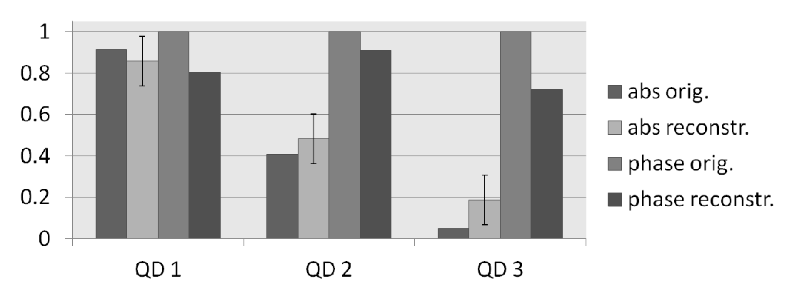
Figure 6: Original and reconstructed coefficients of single-exciton wave function $e_{2}$: Phase in multiples of $2\pi$. Error of absolute values determined by localization.

To demonstrate the success of the tomography, we compare in Fig. 6 the elements of the reconstructed wavefunction for the strongest contribution, i.e. state $e_{2}$ (marked with A in Fig. 5a)), to the original wave function resulting from the input parameters in the Hamiltonian. The agreement for both the amplitude and the relative phase is quite good. The difference results from a non-perfect localization $E^{1}_{i}(\mathbf{r}_{j},\omega_{eg})\neq\delta_{ij}E^{1}_{i}(\mathbf{r}_{i},\omega_{eg})$ resulting from realistic Maxwell simulation from section III.1. This error is marked by the error bars in Fig. 6. It is caused by a weak excitation of quantum dots, which a ideally localized pulse should not excite. Such a non ideal excitation leads to a cross talk between the coefficients. The error bars are estimated to be smaller than: $\Delta_{c^{e}_{i}}=\sum_{j\neq i}|E_{i}(\mathrm{r}_{j})|/|E_{i}(\mathrm{r}_{i})|$.

Note, that in general, the procedure works also for other methods than heterodyne detection in far field, including a localized detection of polarisation or fluorescence, as long as the detection is the same for a localization of the first pulse at different quantum dots. The only limitation is, that the phase of the coefficients can only be detected with methods, that can measure complex signals. For other types of detection like homodyne detection, we can also extract the absolute value of the coefficients, but not their phase.

V Filtering coherent spectra

As additional useful application, we show that strong, undesired resonances can be selectively suppressed from coherent spectra. This can be advantageous while investigating weak resonances, that are masked by other strong resonances: Often, it is not clear, whether weak resonances constitute a vibrational side peak connected to a dominanting strong excitonic peak or a different, much weaker excitonic resonance. This can also be solved by selectively removing excitonic resonances from measured spectra, applying a filter algorithm.
As input information for the filter algorithm, we have to determine expansion coefficients $c^{e_{\alpha}}_{i}$ for the specific state $e_{\alpha}$ for all quantum dots $i$, whose contributions we want to filter out. Additionally, we need all dipole moments $\mu_{gi}$ of the individual nanostructure and also the electric field along the local dipole $\mu_{gi}^{*}\cdot E_{i}^{1}(\mathbf{r}_{i},\omega_{eg})$.
As measurement we record a localized version of the spectrum to be filtered. The localized pulse should excite a ground state to single exciton transition for all quantum dot positions. For the double quantum coherence, this will be the signal $S_{k_{III}}(i,\Omega_{1},\Omega_{2},t_{3})$ for every quantum dot $i$.
For postprocessing we discuss the expression

$$S_{k_{III},w/oe_{\alpha}}(\Omega_{1},\Omega_{2},t_{3})$$

$$\qquad=S_{k_{III}}(\Omega_{1},\Omega_{2},t_{3})-\sum_{i}{c_{i}^{e_{\alpha}}}^{*}\mu_{ig}^{*}\cdot E^{1}(\omega_{eg})f_{e_{\alpha}}(\Omega_{1},\Omega_{2},t_{3})$$

$$\qquad=\sum_{e^{\prime}\neq e_{\alpha},i}{c_{i}^{e^{\prime}}}^{*}\mu_{ig}^{*}\cdot E_{i}^{1}(\omega_{eg})f_{e^{\prime}}(\Omega_{1},\Omega_{2},t_{3})$$ (26)

$$f_{e_{\alpha}}(\Omega_{1},\Omega_{2},t_{3})=\sum_{i}c^{e_{\alpha}}_{i}S_{k_{III}}(i,\Omega_{1},\Omega_{2},t_{3})/(\mu_{ig}^{*}\cdot E_{i}^{1}(\mathbf{r}_{i},\omega_{eg}))$$ (27)

which gives a spectrum, where all contribution of $e_{\alpha}$ during the first pulse are filtered out.

The single-exciton peak $e_{2}$ ($\alpha=2$) dominating the spectrum in Fig. 5 a) is filtered out in Fig. 5d). This spectrum reveals now information about states initially covered by the dominant contribution of $e_{2}$. The procedure can be applied iteratively, using the filtered spectra for obtaining the other excitonic states. This can enhance the reconstruction of the exciton states.

The filtering method can also be applied to other spectroscopic signals as long as a phase sensible detection is used and a localized signal, whose contributions are proportional to the single exciton expansion coefficients, can be measured.

VI Conclusion and outlook

The presented quantum state tomography for the extraction of the delocalized single exciton wave function coefficients, can also be applied to other impulsive two dimensional spectra. The single-exciton to two-exciton transition in double quantum coherence using the localization of the second pulse also also can be used to extract the two exciton coefficients. However since this problem is more complex, it will be subject to future work.

In conclusion, our simulations demonstrate a quantum state tomography that can be used to reconstruct individual wave functions of coupled emitters acting only collectively in the far field. In addition, localized excitations are useful to remove unwanted strong resonances to uncover weak or hidden excitonic resonances. All of these features are not accessible in standard far field spectroscopy. Similar configurations can be alternatively achieved by applying four pulses and using phase cycling to detect a desired componentBrinks et al. (2010) e.g. with phase $\varphi=\varphi_{1}+\varphi_{2}-\varphi_{3}-\varphi_{4}$. We therefore believe that the proposed quantum state tomography opens a new path for the detection of many body interactions on the nanoscale. The proposed protocol is more general as presented here, since fluorescence can also be used rather than heterodyne detection of optical fields Brinks et al. (2010).