Weak Informativity and the Information in One Prior Relative to Another

Abstract

A question of some interest is how to characterize the amount of information that a prior puts into a statistical analysis. Rather than a general characterization, we provide an approach to characterizing the amount of information a prior puts into an analysis, when compared to another base prior. The base prior is considered to be the prior that best reflects the current available information. Our purpose then is to characterize priors that can be used as conservative inputs to an analysis relative to the base prior. The characterization that we provide is in terms of a priori measures of prior-data conflict.

and

1 Introduction

Suppose we have two proper priors $\Pi_{1}$ and $\Pi_{2}$ on a parameter space $\Theta$ for a statistical model $\{P_{\theta}\dvtx\theta\in\Theta\}$. A natural question to ask is: how do we compare the amount of information each of these priors puts into the problem? While there may seem to be natural intuitive ways to express this, such as prior variances, it seems difficult to characterize this precisely in general. For example, the consideration of several examples in Sections 3 and 4 makes it clear that using the variance of the prior is not appropriate for this task.

The motivation for this work comes from Gelman (2006) and Gelman et al. (2008), where the intuitively satisfying notion of weakly informative priors is introduced as a compromise between informative and noninformative priors. The basic idea is that we have a base prior $\Pi_{1}$, perhaps elicited, that we believe reflects our current information about $\theta$, but we choose to be conservative in our inferences and select a prior $\Pi_{2}$ that puts less information into the analysis. While it is common to take $\Pi_{2}$ to be a noninformative prior, this can often produce difficulties when $\Pi_{2}$ is improper, and even when $\Pi_{2}$ is proper, it seems inappropriate, as it completely discards the information we have about $\theta$ as expressed in $\Pi_{1}$. In addition, we may find that a prior-data conflict exists with $\Pi_{1}$ and so look for another prior that reflects at least some of the information that $\Pi_{1}$ puts into an analysis, but avoids the conflict.

We note that our discussion here is only about how we should choose $\Pi_{2}$ given that $\Pi_{1}$ has already been chosen. Of course, the choice of $\Pi_{1}$ is of central importance in a Bayesian analysis. Ideally, $\Pi_{1}$ is chosen based on a clearly justified elicitation process, but we know that this is often not the case. In such a circumstance it makes sense to try and choose $\Pi_{1}$ reasonably but then be deliberately less informative by choosing $\Pi_{2}$ to be weakly informative with respect to $\Pi_{1}$. The point is to inspire confidence that our analysis is not highly dependent on information that may be unreliable. To do this, however, requires a definition of what it means for one prior to be weakly informative with respect to another and that is what this paper is about.

To implement the idea of weak informativity, we need a precise definition. We provide this in Section 2 and note that it involves the notion of prior-data conflict. Intuitively, a prior-data conflict occurs when the prior places the bulk of its mass where the likelihood is relatively low, as the likelihood is indicating that the true value of the parameter is in the tails of the prior. Our definition of weak informativity is then expressed by saying that $\Pi_{2}$ is weakly informative relative to $\Pi_{1}$ whenever $\Pi_{2}$ produces fewer prior-data conflicts a priori than $\Pi_{1}$. This leads to a quantifiable expression of weak informativity that can be used to choose priors. In Section 3 we consider this definition in the context of several standard families of priors and it is seen to produce results that are intuitively reasonable. In Section 4 we consider applications of this concept in some data analysis problems. While our intuition about weak informativity is often borne out, we also find that in certain situations we have to be careful before calling a prior weakly informative.

First, however, we establish some notation and then review how we check for prior-data conflict. We suppose that $P_{\theta}(A)=\int_{A}f_{\theta}(x)\mu(dx)$, that is, each $P_{\theta}$ is absolutely continuous with respect to a support measure $\mu$ on the sample space $\mathcal{X}$, with the density denoted by $f_{\theta}$. With this formulation a prior $\Pi$ leads to a prior predictive probability measure on $\mathcal{X}$ given by $M(A)=\int_{\Theta}P_{\theta}(A)\Pi(d\theta)=\int_{A}m(x)\mu(dx)$, where $m(x)=\int_{\Theta}f_{\theta}(x)\Pi(d\theta)$. If $T$ is a minimal sufficient statistic for $\{P_{\theta}\dvtx\theta\in\Theta\}$, then it is well known that the posterior is the same whether we observe $x$ or $T(x)$. So we will denote the posterior by $\Pi(\cdot|T)$ hereafter. Since $T$ is minimal sufficient, we know that the conditional distribution of $x$ given $T$ is independent of $\theta$. We denote this conditional measure by $P(\cdot|T)$. The joint distribution $P_{\theta}\times\Pi$ can then be factored as

$$P_{\theta}\times\Pi = M\times\Pi(\cdot|x)$$

$$= P(\cdot|T)\times M_{T}\times\Pi(\cdot|T),$$

where $M_{T}$ is the marginal prior predictive distribution of $T$.

While much of Bayesian analysis focuses on the third factor in (1), there are also roles in a statistical analysis for $P(\cdot|T)$ and $M_{T}$. As discussed in Evans and Moshonov (2006, 2007), $P(\cdot|T)$ is available for checking the sampling model, for example, if $x$ is a surprising value from this distribution, then we have evidence that the model $\{P_{\theta}\dvtx\theta\in\Theta\}$ is incorrect. Furthermore, it is argued that, if we conclude that we have no evidence against the model, then the factor $M_{T}$ is available for checking whether or not there is any prior-data conflict, and we do this by comparing the observed value of $T(x)$ to $M_{T}$. If we have no evidence against the model, and no evidence of prior-data conflict, then we can proceed to inferences about $\theta$. Actually, the issues involved in model checking and checking for prior-data conflict are more involved than this (see, e.g., the cited references and Section 5), but (1) gives the basic idea that the full information, as expressed by the joint distribution of $(\theta,x)$, splits into components, each of which is available for a specific purpose in a statistical analysis.

Accordingly, we restrict ourselves here, for any discussions concerning prior-data conflict, to working with $M_{T}$. One issue that needs to be addressed is how one is to compare the observed value $t_{0}=T(x_{0})$ to $M_{T}$. In essence, we need a measure of surprise and for this we use a $P$-value. Effectively, we are in the situation where we have a value from a single fixed distribution and we need to specify the appropriate $P$-value to use. In Evans and Moshonov (2006, 2007) the $P$-value for checking for prior-data conflict is given by

$$M_{T}\bigl{(}m_{T}(t)\leq m_{T}(t_{0})\bigr{)},$$ (2)

where $m_{T}$ is the density of $M_{T}$ with respect to the volume measure on the range space for $T$. In Evans and Jang (2011) it is proved that, for many of the models and priors used in statistical analyses, (2) converges almost surely, as the amount of data increases, to $\Pi(\pi(\theta)\leq\pi(\theta_{*}))$, where $\theta_{*}$ is the true value of $\theta$. So (2) is assessing to what extent the true value is in the tails of the prior, or, equivalently, to what extent the prior information is in conflict with how the data is being generated.

A difficulty with (2) is that it is not generally invariant to the choice of the minimal sufficient statistic $T$. A general invariant $P$-value is developed in Evans and Jang (2010) for situations where we want to compare the observed value of a statistic to a fixed distribution. This requires that the model and $T$ satisfy some regularity conditions, for example, all spaces need to be locally Euclidean, support measures are given by volume measures on these spaces, and $T$ needs to be sufficiently smooth. A formal description of these conditions can be found in Tjur (1974) and it is noted that these hold for the typical statistical application. For example, these conditions are immediately satisfied in the discrete case. Furthermore, for continuous situations, with densities defined as limits, we get the usual expressions for densities. When applied to checking for prior-data conflict, this leads to using the invariant $P$-value

$$M_{T}\bigl{(}m_{T}^{\ast}(t)\leq m_{T}^{\ast}(t_{0})\bigr{)},$$ (3)

where $m_{T}^{\ast}(t)=\int_{T^{-1}{t}}m(x)\mu_{T^{-1}\{t\}}(dx)=m_{T}(t)\cdot\break E(J_{T}^{-1}(x)|T(x)=t)$, $\mu_{T^{-1}\{t\}}$ is the volume measure on $T^{-1}\{t\}$, $J_{T}(x)=(\det(dT(x)\circ dT^{\prime}(x)))^{-1/2}$ and $dT$ is the differential of $T$. Note that $J_{T}(x)$ gives the volume distortion produced by $T$ at $x$. So $m_{T}^{\ast}$ is the density of $M_{T}$ with respect to the support measure given by $\{E(J_{T}^{-1}(x)|T(x)=t)\}^{-1}$ times the volume measure on the range space for $T$.

In applications all models are effectively discrete, as we measure responses to some finite accuracy, and continuous models are viewed as being approximations. The use of (3), rather than (2), then expresses the fact that we do not want volume distortions induced by a transformation to affect our inferences. So we allocate this effect of the transformation with the support measure, rather than with the density, when computing the $P$-value. In the discrete case, as well as when $T$ is linear, (2) and (3) give the same value and otherwise seem to give very similar values. Convergence of (3), to an invariant $P$-value based on the prior, is established in Evans and Jang (2011). We use (3) throughout this paper but note that it is only in Section 3.3 where (3) differs from (2).

Our discussion here is based on a minimal sufficient statistic $T$. We note that, except in mathematically pathological situations, such a statistic exists. It may be, however, that $T$ is high dimensional, for example, $T$ can be of the same dimension as the data. In such situations the dimensionality of the problem can often be reduced by examining components of the prior in a hierarchical fashion. For example, when the prior on $\theta=(\theta_{1},\theta_{2})$ is specified as $\pi(\theta)=\pi_{2}(\theta_{2}|\theta_{1})\pi_{1}(\theta_{1})$, then $\pi_{1}$ and $\pi_{2}(\cdot|\theta_{1})$ are checked separately and so the definition of weak informativity applies to each component separately. This is exemplified by the regression example of Section 4.2 where $\theta=(\theta_{1},\theta_{2})=(\beta,\sigma^{2})$. More on checking the components of a prior can be found in Evans and Moshonov (2006). Furthermore, when ancillaries exist, it is necessary to condition on these when checking for prior-data conflict, as this variation has nothing to do with the prior. This results in a reduction of the dimension of the problem. The relevance of ancillarity to the problem of weakly informative priors is discussed in Section 5.

When choosing a prior it makes sense to consider the prior distribution of more than just the minimal sufficient statistic. For example, Chib and Ergashev (2009) consider the prior distribution of a somewhat complicated function of the parameters and data that has a real world interpretation. If this distribution produces values that seem reasonable in light of what is known, then this goes some distance toward justifying the prior. Also, the level of informativity of the prior can be judged by looking at the prior distribution of this quantity when that is possible. While this is certainly a reasonable approach to choosing $\Pi_{1}$, it does not supply us with a definition of weak informativity. For example, a prior $\Pi_{1}$ can be chosen as discussed in Chib and Ergashev (2009), but then $\Pi_{2}$ could be chosen to be weakly informative with respect to $\Pi_{1}$, to inspire confidence that conclusions drawn are not highly dependent on subjective appraisals.

As we will show, there will typically be many priors $\Pi_{2}$ that are weakly informative with respect to a given base prior $\Pi_{1}$. The question then arises as to which $\Pi_{2}$ we should use. This is partially answered in Section 2 where we show that the definition of weak informativity leads to a quantification of how much less informative $\Pi_{2}$ is than $\Pi_{1}$. For example, we can choose $\Pi_{2}$ in a family of priors to be 50% less informative than $\Pi_{1}$. Still, there may be many such $\Pi_{2}$ and at this time we do not have a criterion that allows us to distinguish among such priors. For example, suppose the base prior is a normal prior for a location parameter. We can derive weakly informative priors with respect to such a prior in the family of normal priors (see Section 3.1) or in the family of $t$ priors (see Section 3.2). There is nothing in our developments that suggests that a weakly informative $t$ prior is to be preferred to a weakly informative normal prior or conversely. Such distinctions will have to be made based on other criteria.

2 Comparing Priors

There are a variety of measures of information used in statistics. Several measures have been based on the concept of entropy, for example, see Lindley (1956) and Bernardo (1979). While these measures have their virtues, we note that their coding theory interpretations can seem somewhat abstract in statistical contexts and they can suffer from nonexistence in certain problems. Also, Kass and Wasserman (1995) contain some discussion concerned with expressing the absolute information content of a prior in terms of additional sample values. Rather than adopting these approaches, we consider comparing priors based on their tendencies to produce prior-data conflicts. This formulation of the relative amount of information put into an analysis has a direct interpretation in terms of statistical consequences.

Suppose that an analyst has in mind a prior $\Pi_{1}$ that they believe represents the information at hand concerning $\theta$. The analyst, however, prefers to use a prior $\Pi_{2}$ that is conservative, when compared to $\Pi_{1}$. In such a situation it seems reasonable to consider $\Pi_{1}$ as a base prior and then compare all other priors to it. This idea comes from Gelman (2006) and leads to the notion of weakly informative priors.

Before we observe data we have no way of knowing if we will have a prior-data conflict. Accordingly, since the analyst has determined that $\Pi_{1}$ best reflects the available information, it is reasonable to consider the prior distribution of $P_{1}(t_{0})=\break M_{1T}(m_{1T}^{\ast}(t)\leq m_{1T}^{\ast}(t_{0}))$ when $t_{0}\sim M_{1T}$. Of course, this is effectively uniformly distributed [exactly so when $m_{1T}^{\ast}(t)$ has a continuous distribution when $t\sim M_{1T}$] and this expresses the fact that all the information about assessing whether or not a prior-data conflict exists is contained in the $P$-value, with no need to compare the $P$-value to its distribution.

Consider now, however, the distribution of $P_{2}(t_{0})\!=M_{2T}(m_{2T}^{\ast}(t)\leq m_{2T}^{*}(t_{0}))$ which is used to check whether or not there is prior-data conflict with respect to $\Pi_{2}$. Given that we have identified that a priori the appropriate distribution of $t_{0}$ is $M_{1T}$, at least for inferences about an unobserved value, then $P_{2}(t_{0})$ is not uniformly distributed. In fact, from the distribution of $P_{2}(t_{0})$ we can obtain an intuitively reasonable idea of what it means for a prior $\Pi_{2}$ to be weakly informative relative to $\Pi_{1}$. Suppose that the prior distribution of $P_{2}(t_{0})$ clusters around 1. This implies that, if we were to use $\Pi_{2}$ as the prior when $\Pi_{1}$ is appropriate, then there is a small prior probability that a prior-data conflict would arise. Similarly, if the prior distribution of $P_{2}(t_{0})$ clusters around 0, then there is a large prior probability that a prior-data conflict would arise. If one prior distribution results in a larger prior probability of there being a prior-data conflict than another, then it seems reasonable to say that the first prior is more informative than the second. In fact, a completely noninformative prior should never produce prior-data conflicts.

So we compare the distribution of $P_{2}(t_{0})$ when $t_{0}\sim M_{1T}$, to the distribution of $P_{1}(t_{0})$ when $t_{0}\sim M_{1T}$, and do this in a way that is relevant to the prior probability of obtaining a prior-data conflict. One approach to this comparison is to select a $\gamma$-quantile $x_{\gamma}\in[0,1]$ of the distribution of $P_{1}(t_{0})$, and then compute the probability

$$M_{1T}\bigl{(}P_{2}(t_{0})\leq x_{\gamma}\bigr{)}.$$ (4)

The value $\gamma$ is presumably some cutoff, dependent on the application, where we will consider that evidence of a prior-data conflict exists whenever$P_{1}(t_{0})\leq\gamma$. Of course, if $m_{1T}^{\ast}(t_{0})$ has a continuous distribution when $t_{0}\sim M_{1T}$, then $x_{\gamma}=\gamma$. Our basic criterion for the weak informativity of $\Pi_{2}$ relative to $\Pi_{1}$ will then be that (4) is less than or equal to $x_{\gamma}$. This implies that the prior probability of obtaining a prior-data conflict under $\Pi_{2}$ is no greater than when $\Pi_{1}$ is used, at least when we have identified $\Pi_{1}$ as our correct prior.

Definition 1.

If (4) is less than or equal to $x_{\gamma}$, then $\Pi_{2}$ is weakly informative relative to $\Pi_{1}$ at level $\gamma$. If $\Pi_{2}$ is weakly informative relative to $\Pi_{1}$ at level $\gamma$ for every $\gamma\leq\gamma_{0}$, then $\Pi_{2}$ is uniformly weakly informative relative to $\Pi_{1}$ at level $\gamma_{0}$. If $\Pi_{2}$ is weakly informative relative to $\Pi_{1}$ at level $\gamma$ for every $\gamma$, then $\Pi_{2}$ is uniformly weakly informative relative to $\Pi_{1}$.

Typically we would like to choose a prior $\Pi_{2}$ that is uniformly weakly informative with respect to $\Pi_{1}$. This still requires us to select a prior from this class, however, and for this we must choose a level $\gamma$.

Once we have selected $\gamma$, the degree of weak informativity of a prior $\Pi_{2}$ relative to $\Pi_{1}$ can be assessed by comparing $M_{1T}(P_{2}(t_{0})\leq x_{\gamma})$ to $x_{\gamma}$ via the ratio

$$1-M_{1T}\bigl{(}P_{2}(t_{0})\leq x_{\gamma}\bigr{)}/x_{\gamma}.$$ (5)

If $\Pi_{2}$ is weakly informative relative to $\Pi_{1}$ at level $\gamma$, then (5) tells us the proportion of fewer prior-data conflicts we can expect a priori when using $\Pi_{2}$ rather than $\Pi_{1}$. Thus, (5) provides a measure of how much less informative $\Pi_{2}$ is than $\Pi_{1}$ at level $\gamma$. So, for example, we might ask for a prior $\Pi_{2}$ that is uniformly weakly informative with respect to $\Pi_{1}$ and then, for a particular $\gamma$, select a prior in this class such that (5) equals 50%.

As we will see in the examples, it makes sense to talk of one prior being asymptotically weakly informative at level $\gamma$ with respect to another prior in the sense that (4) is bounded above by $\gamma$ in the limit as the amount of data increases. In several cases this simplifies matters considerably, as an asymptotically weakly informative prior is easy to find and may still be weakly informative for finite amounts of data.

While (4) seems difficult to work with, the following result is proved in the Appendix and gives a simpler expression.

Lemma 1.

Suppose $P_{i}(t)$ has a continuous distribution under $M_{iT}$ for $i=1,2$. Then there exists $r_{\gamma}$ such that $M_{1T}(P_{2}(t)\leq\gamma)=M_{1T}(m_{2T}^{\ast}(t)\leq r_{\gamma})$, and $\Pi_{2}$ is weakly informative at level $\gamma$ relative to $\Pi_{1}$ whenever $M_{1T}(m_{2T}^{\ast}(t)\leq r_{\gamma})\leq\gamma$. Furthermore, $\Pi_{2}$ is uniformly weakly informative relative to $\Pi_{1}$ if and only if $M_{1T}(m_{2T}^{\ast}(t)\leq m_{2T}^{\ast}(t_{0}))\leq M_{2T}(m_{2T}^{\ast}(t)\leq\break m_{2T}^{\ast}(t_{0}))$ for every $t_{0}$.

Note that the equivalent condition for uniform weak informativity in Lemma 1 says that the probability content, under $M_{1T}$, in the “tails” (regions of low density) of the density $m_{2T}^{\ast}$ is always bounded above by the probability content under $M_{2T}$. So $M_{2T}$ puts more probability content into these tails than $M_{1T}$ and this can be taken as an indication that $M_{2T}$ is more dispersed than $M_{1T}$. Lemma 1 typically applies when we are dealing with continuous distributions on $\mathcal{X}$. It can also be shown that $P_{i}(t)$ has a continuous distribution under $M_{iT}$ if and only if $m_{iT}^{\ast}(t)$ has a continuous distribution under $M_{iT}$.

3 Deriving Weakly Informative Priors

We consider several examples of families of priors that arise in applications. These examples support our definition of weak informativity and also lead to some insights into choosing priors. The results obtained for the examples in this section are combined in Section 4.2 to give results for a practically meaningful context.

We first note that, while we could consider comparing arbitrary priors $\Pi_{2}$ to $\Pi_{1}$, we want $\Pi_{2}$ to reflect at least some of the information expressed in $\Pi_{1}$. The simplest expression of this is to require that $\Pi_{2}$ have the same, or nearly the same, location as $\Pi_{1}$. This restriction simplifies the analysis and seems natural.

3.1 Comparing Normal Priors

Suppose we have a sample $x=(x_{1},\ldots,x_{n})$ from a $N(\mu,1)$ distribution where $\mu$ is unknown. Then $t=T(x)=\bar{x}\sim N(\mu,1/n)$ is minimal sufficient and since $T$ is linear, there is constant volume distortion and so this can be ignored. Suppose that the prior $\Pi_{1}$ on $\mu$ is a $N(\mu_{0},\sigma_{1}^{2})$ distribution with $\mu_{0}$ and $\sigma_{1}^{2}$ known. We then have that $M_{1T}$ is the $N(\mu_{0},1/n+\sigma_{1}^{2})$ distribution. Now suppose that $\Pi_{2}$ is a $N(\mu_{0},\sigma_{2}^{2})$ distribution with $\sigma_{2}^{2}$ known. Then $M_{2T}$ is the $N(\mu_{0},\break 1/n+\sigma_{2}^{2})$ distribution and

$$P_{2}(t_{0}) = M_{2T}\bigl{(}m_{2T}^{\ast}(t)\leq m_{2T}^{\ast}(t_{0})\bigr{)}$$

$$= M_{2T}\bigl{(}m_{2T}(t)\leq m_{2T}(t_{0})\bigr{)}$$

$$= M_{2T}\bigl{(}(t-\mu_{0})^{2}\geq(t_{0}-\mu_{0})^{2}\bigr{)}$$

$$= 1-G_{1}\bigl{(}(t_{0}-\mu_{0})^{2}/(1/n+\sigma_{2}^{2})\bigr{)},$$

where $G_{k}$ denotes the $\operatorname{Chi\mbox{-}squared}(k)$ distribution function. Now under $M_{1T}$ we have that $(t_{0}-\mu_{0})^{2}/\break(1/n+\sigma_{1}^{2})\sim\operatorname{Chi\mbox{-}squared}(1)$. Therefore,

$$M_{1T}\bigl{(}P_{2}(t_{0})\leq\gamma\bigr{)}$$

$$\quad=M_{1T}\bigl{(}1-G_{1}\bigl{(}(t_{0}-\mu_{0})^{2}/(1/n+\sigma_{2}^{2})\bigr{)}\leq\gamma\bigr{)}$$

$$\quad=M_{1T}\biggl{(}\frac{(t_{0}-\mu_{0})^{2}}{1/n+\sigma_{1}^{2}}\geq\frac{1/n+\sigma_{2}^{2}}{1/n+\sigma_{1}^{2}}G_{1}^{-1}(1-\gamma)\biggr{)}$$

$$\quad=1-G_{1}\biggl{(}\frac{1/n+\sigma_{2}^{2}}{1/n+\sigma_{1}^{2}}G_{1}^{-1}(1-\gamma)\biggr{)}.$$

We see immediately that (3.1) will be less than $\gamma$ if and only if $\sigma_{2}>\sigma_{1}$. In other words, $\Pi_{2}$ will be uniformly weakly informative relative to $\Pi_{1}$ if and only if $\Pi_{2}$ is more diffuse than $\Pi_{1}$. Note that $M_{1T}(P_{2}(t_{0})\leq\gamma)$ converges to 0 as $\sigma_{2}^{2}\rightarrow\infty$ to reflect noninformativity. Also, as $n\rightarrow\infty$, then (3.1) increases to $1-G_{1}((\sigma_{2}^{2}/\sigma_{1}^{2})G_{1}^{-1}(1-\gamma))$. So we could ignore $n$ and choose $\sigma_{2}^{2}$ conservatively based on this limit, to obtain an asymptotically uniformly weakly informative prior, as we know this value of $\sigma_{2}^{2}$ will also be weakly informative for finite $n$.

If we specify that we want (5) to equal $p\in[0,1]$, then (3.1) implies that $\sigma_{2}^{2}=(1/n+\sigma_{1}^{2})(G_{1}^{-1}(1-\gamma+p\gamma)/G_{1}^{-1}(1-\gamma))-1/n$. Such a choice will give a proportion $p$ fewer prior-data conflicts at level $\gamma$ than the base prior. This decreases to $\sigma_{1}^{2}G_{1}^{-1}(1-\gamma+p\gamma)/G_{1}^{-1}(1-\gamma)$ as $n\rightarrow\infty$ and so the more data we have the less extra variance we need for $\Pi_{2}$ for weak informativity.

We can generalize this to $t\sim N_{k}(\mu,n^{-1}I)$ with $\Pi_{i}$ given by $\mu\sim N_{k}(\mu_{0},\Sigma_{i})$. Note we have that $M_{iT}$ is the $N_{k}(\mu_{0},n^{-1}I+\Sigma_{i})$ distribution. It is then easy to see that $P_{2}(t_{0})=1-G_{k}((t_{0}-\mu_{0})^{\prime}(n^{-1}I+\Sigma_{2})^{-1}(t_{0}-\mu_{0}))$ and

$$M_{1T}\bigl{(}P_{2}(t_{0})\leq\gamma\bigr{)}$$

$$\quad=M_{1T}\bigl{(}(t_{0}-\mu_{0})^{\prime}(n^{-1}I+\Sigma_{2})^{-1}(t_{0}-\mu_{0})$$

$$\quad\hskip 125.0pt\geq G_{k}^{-1}(1-\gamma)\bigr{)}.$$

Note that (3.1) increases to the probability that $(t_{0}-\mu_{0})^{\prime}\Sigma_{2}{}^{-1}(t_{0}-\mu_{0})\geq G_{k}^{-1}(1-\gamma)$, when $t_{0}\sim N_{k}(\mu_{0},\Sigma_{1})$, as $n\rightarrow\infty$. This probability can be easily computed via simulation.

The following result is proved in the Appendix.

Theorem 1.

For a sample of $n$ from the statistical model $\{N_{k}(\mu,I)\dvtx\mu\in R^{k}\}$, a $N_{k}(\mu_{0},\Sigma_{2})$ prior is uniformly weakly informative relative to a $N_{k}(\mu_{0},\Sigma_{1})$ prior if and only if $\Sigma_{2}-\Sigma_{1}$ is positive semidefinite.

The necessary part of Theorem 1 is much more difficult than the $k=1$ case and shows that we cannot have a $N_{k}(\mu_{0},\Sigma_{2})$ prior uniformly weakly informative relative to a $N_{k}(\mu_{0},\Sigma_{1})$ prior unless $\Sigma_{2}\geq\Sigma_{1}$. It follows from Theorem 1 that a $N_{k}(\mu_{0},\Sigma_{2})$ prior is uniformly weakly informative relative to a $N_{k}(\mu_{0},\Sigma_{1})$ prior if and only if a $N(a^{t}\mu_{0},a^{t}\Sigma_{2}a)$ prior is uniformly weakly informative relative to a $N(a^{t}\mu_{0},a^{t}\Sigma_{1}a)$ prior for every $a\in R^{k}$.

For the choice of $\Sigma_{2}$ we have that, if $\Sigma_{1}$ and $\Sigma_{2}$ are arbitrary $k\times k$ positive definite matrices, then $r\Sigma_{2}\geq\Sigma_{1}$ whenever $r\geq\lambda_{k}(\Sigma_{1})/\lambda_{1}(\Sigma_{2})$ where $\lambda_{i}(\Sigma)$ denotes the $i$th ordered eigenvalue of $\Sigma$. Note that this condition does not require that the $\Sigma_{i}$ have the same eigenvectors. When they do have the same eigenvectors, so $\Sigma_{i}=QD_{i}Q^{\prime}$ is the spectral decomposition of $\Sigma_{i}$, then $\Sigma_{2}\geq\Sigma_{1}$ whenever $\lambda_{i}(\Sigma_{2})\geq\lambda_{i}(\Sigma_{1})$ for $i=1,\ldots,k$.

3.2 Comparing a $t$ Prior with a Normal Prior

It is not uncommon to find $t$ priors being substituted for normal priors on location parameters. Suppose $x=(x_{1},\ldots,x_{n})$ is a sample from a $N(\mu,1)$ distribution where $\mu$ is unknown. We take $\Pi_{1}$ to be a $N(\mu_{0},\sigma_{1}^{2})$ distribution and $\Pi_{2}$ to be a $t_{1}(\mu_{0},\sigma_{2}^{2},\lambda)$ distribution, that is, $t_{1}(\mu_{0},\sigma_{2}^{2},\lambda)$ denotes the distribution of $\mu_{0}+\sigma_{2}z$ with $z$ distributed as a 1-dimensional $t$ distribution with $\lambda$ degrees of freedom. We then want to determine $\sigma_{2}^{2}$ and $\lambda$ so that the $t_{1}(\mu_{0},\sigma_{2}^{2},\lambda)$ prior is weakly informative relative to the normal prior.

We consider first the limiting case as $n\rightarrow\infty$. The limiting prior predictive distribution of the minimal sufficient statistic $T(x)=\bar{x}$ is $N(\mu_{0},\sigma_{1}^{2})$ while $P_{2}(t_{0})$ converges in distribution to $1-H_{1,\lambda}((t_{0}-\mu_{0})^{2}/\sigma_{2}^{2})$ where $H_{1,\lambda}$ is the distribution function of an $F_{1,\lambda}$ distribution. This implies that (4) converges to $1-G_{1}((\sigma_{2}^{2}/\sigma_{1}^{2})H_{1,\lambda}^{-1}(1-\gamma))$ and this is less than or equal to $\gamma$ if and only if $\sigma_{2}^{2}/\sigma_{1}^{2}\geq G_{1}^{-1}(1-\gamma)/H_{1,\lambda}^{-1}(1-\gamma))$. So to have that $\Pi_{2}$ is asymptotically weakly informative relative to $\Pi_{1}$ at level $\gamma$, we must choose $\sigma_{2}^{2}$ large enough. Clearly we have that $\Pi_{2}$ is asymptotically uniformly weakly informative relative to $\Pi_{1}$ if and only if

$$\sigma_{2}^{2}/\sigma_{1}^{2}\geq K(\lambda)=\sup_{\gamma\in[0,1]}G_{1}^{-1}(1-\gamma)/H_{1,\lambda}^{-1}(1-\gamma).$$

In Figure 1 we have plotted $K(\lambda)$ against $\log(\lambda)$.

Figure 1: Plot of $K(\lambda)$ against $\log(\lambda)$ where a $t_{1}(\mu_{0},\sigma_{2}^{2},\lambda)$ prior is asymptotically uniformly weakly informative relative to a $N(\mu_{0},\sigma_{1}^{2})$ prior if and only if $\sigma_{2}^{2}/\sigma_{1}^{2}\geq K(\lambda)$.

Since $K(1)=0.6366$, we require that $\sigma_{2}^{2}\geq\break\sigma_{1}^{2}(0.6366)$ for a Cauchy prior to be uniformly weakly informative with respect to a $N(\mu_{0},\sigma_{1}^{2})$ prior.A $t_{1}(\mu_{0},\sigma_{2}^{2},3)$ prior has variance $3\sigma_{2}^{2}$. If we choose $\sigma_{2}^{2}$ so that the variance is $\sigma_{1}^{2}$, then $\sigma_{2}^{2}/\sigma_{1}^{2}=1/3$. Since this is less than $K(3)=0.8488$, this prior is not uniformly weakly informative. A $t_{1}(\mu_{0},\sigma_{2}^{2},3)$ prior has to have variance at least equal to $(2.5464)\sigma_{1}^{2}$ if we want it to be uniformly weakly informative relative to a $N(\mu_{0},\sigma_{1}^{2})$ prior. This is somewhat surprising and undoubtedly is caused by the peakedness of the $t$ distribution. Note that $K(\lambda)\rightarrow 1$ as $\lambda\rightarrow\infty$, so this increase in variance, for the $t$ prior over the normal prior, decreases as we increase the degrees of freedom.

The situation for finite $n$ is covered by the following result proved in the Appendix.

Theorem 2.

For a sample of $n$ from the statistical model $\{N(\mu,1)\dvtx\mu\in R^{1}\}$, a $t_{1}(\mu_{0},\sigma_{2}^{2},\lambda)$ prior is uniformly weakly informative relative to a $N_{1}(\mu_{0},\sigma_{1}^{2})$ prior whenever $\sigma_{2}^{2}\geq\sigma_{0n}^{2}$, where $\sigma_{0n}^{2}$ is the unique solution of $(1/n+\sigma_{1}^{2})^{-1/2}=\int_{0}^{\infty}(1/n+\sigma_{0n}^{2}/u)^{-1/2}\cdot k_{\lambda}(u)\,du$ with $k_{\lambda}$ the $\operatorname{Gamma}_{\mathrm{rate}}(\lambda/2,\lambda/2)$ density. Further, $\sigma_{0n}^{2}/\sigma_{1}^{2}$ increases to

$$\quad K(\lambda)=\sup_{\gamma\in[0,1]}\frac{G_{1}^{-1}(1-\gamma)}{H_{1,\lambda}^{-1}(1-\gamma)}=\frac{2}{\lambda}\frac{\Gamma^{2}((\lambda+1)/2)}{\Gamma^{2}(\lambda/2)}$$ (8)

as $n\rightarrow\infty$ and so a $t_{1}(\mu_{0},\sigma_{2}^{2},\lambda)$ prior is asymptotically uniformly weakly informative if and only if $\sigma_{2}^{2}/\sigma_{1}^{2}$ is greater than or equal to (8).

Theorem 2 establishes that we can conservatively use (8) to select a uniformly weakly informative $t$ prior.

In Figure 2 we have plotted the value of (4) that arises with $t_{1}(0,\sigma_{2}^{2},3)$ priors, where $\sigma_{2}^{2}$ is chosen in a variety of ways, together with the 45-degree line. A uniformly weakly informative prior will have (4) always below the 45-degree line, while a uniformly weakly informative prior at level $\gamma_{0}$ will have (4) below the 45-degree line to the left of $\gamma_{0}$ and possibly above to the right of $\gamma_{0}$. For example, when $\sigma_{2}^{2}=1/3$, then the $t_{1}(0,\sigma_{2}^{2},3)$ prior and the $N(0,1)$ prior have the same variance. We see that this prior is only uniformly weakly informative at level $\gamma_{0}=0.0357$ and is not uniformly weakly informative.

Figure 2: Plot of (4) versus $\gamma$ for $t_{1}(0,\sigma_{2}^{2},3)$ priors relative to a $N(0,1)$ prior when $n=20$, where $\sigma_{2}^{2}$ is chosen to match variances (thick solid line), match the MAD (dashed line), just achieve uniform weak informativity (dotted line), just achieve asymptotic uniform weak informativity (dash-dot line), and equal to 1 (long-dashed line).

Note that (5) converges to $1-G_{1}((\sigma_{2}^{2}/\sigma_{1}^{2})H_{1,\lambda}^{-1}(1-\gamma))/\gamma$ as $n\rightarrow\infty$, and setting this equal to $p$ implies that $\sigma_{2}^{2}=\sigma_{1}^{2}G_{1}^{-1}(1-\gamma+\gamma p)/H_{1,\lambda}^{-1}(1-\gamma)$ which converges, as $\lambda\rightarrow\infty$, to the result we obtained in Section 3.1. So when $\lambda=3,\gamma=0.05$ and $p=0.5$, we must have $\sigma_{2}^{2}/\sigma_{1}^{2}=5.0239/10.1280=0.49604$.

Our analysis indicates that one has to be careful about the scaling of the $t$ prior if we want to say that the $t$ prior is less informative than a normal prior, at least when we want uniform weak informativity.

Consider now comparing a multivariate $t$ prior to a multivariate normal prior. Let $t_{k}(\mu_{0},\Sigma_{2},\lambda)$ denote the $k$-dimensional $t$ distribution given by $\mu_{0}+\Sigma_{2}^{1/2}z$, where $\Sigma_{2}^{1/2}$ is a square root of the positive definite matrix $\Sigma_{2}$ and $z$ has a $k$-dimensional $t$ distribution with $\lambda$ degrees of freedom. This is somewhat more complicated than the normal case, but we prove the following result in the Appendix which provides sufficient conditions for the asymptotic uniform weak informativity.

Theorem 3.

When sampling from the statistical model $\{N_{k}(\mu,I)\dvtx\mu\in R^{k}\}$, a $t_{k}(\mu_{0},\Sigma_{2},\lambda)$ prior is asymptotically uniformly weakly informative relative to a $N_{k}(\mu_{0},\Sigma_{1})$ prior whenever $\Sigma_{2}-\tau_{\lambda}^{2}\Sigma_{1}$ is positive semidefinite, where $\tau_{\lambda}^{2}=(2/\lambda)\Gamma^{2/k}((k+\lambda)/2)/\allowbreak\Gamma^{2/k}(\lambda/2)$.

In contrast with Theorem 1, we do not have an equivalent characterization of the uniform weak informativity of multivariate $t$ priors in terms of the marginal priors of $a^{t}\mu$. For example, when $k=2$, then $\tau_{\lambda}^{2}\,{=}\,1$ and when $k\,{=}\,1$, then $\tau_{\lambda}^{2}\,{=}\,2\Gamma^{2}((\lambda\,{+}\,1)/2)/\break\lambda\Gamma^{2}(\lambda/2)<1$ for all $\lambda$. Therefore, $a^{t}\Sigma_{2}a-\{2\Gamma^{2}((\lambda+1)/2)/\lambda\Gamma^{2}(\lambda/2)\}a^{t}\Sigma_{1}a>0$ for all $a$ does not imply that $\Sigma_{2}-\Sigma_{1}$ is positive semidefinite, for example, take $\Sigma_{2}=\Sigma_{1}(1+2\Gamma^{2}((\lambda+1)/2)/\lambda\Gamma^{2}(\lambda/2))/2$.

For the choice of $\Sigma_{2}$ we have that, if $\Sigma_{1}$ and $\Sigma_{2}$ are arbitrary $k\times k$ positive definite matrices, then $r\Sigma_{2}\geq\tau_{\lambda}^{2}\Sigma_{1}$ whenever $r\geq\tau_{\lambda}^{2}\lambda_{k}(\Sigma_{1})/\lambda_{1}(\Sigma_{2})$. When the $\Sigma_{i}$ have the same eigenvectors, then $\Sigma_{2}\geq\tau_{\lambda}^{2}\Sigma_{1}$ whenever $\lambda_{i}(\Sigma_{2})\geq\tau_{\lambda}^{2}\lambda_{i}(\Sigma_{1})$ for $i=1,\ldots,k$.

3.3 Comparing Inverse Gamma Priors

Suppose now that we have a sample $x\,{=}\,(x_{1},\ldots,x_{n})$ from a $N(0,\sigma^{2})$ distribution where $\sigma^{2}$ is unknown. Then $t=T(x)=(x_{1}^{2}+\cdots+x_{n}^{2})/n$ is minimal sufficient and $T\sim\operatorname{Gamma}_{\mathrm{rate}}(n/2,n/2\sigma^{2})$. Now suppose that we take $\Pi_{i}$ to be an inverse gamma prior on $\sigma^{2}$, namely, $\sigma^{-2}\sim\operatorname{Gamma}_{\mathrm{rate}}(\alpha_{i},\beta_{i})$. From this we get that $\alpha_{i}T/\beta_{i}\sim F(n,2\alpha_{i})$ and, since $J_{T}(x)=(4x^{\prime}x/\break n)^{-1/2}=(4t/n)^{-1/2},m_{iT,n}^{\ast}(t)=m_{iT,n}(t)\cdot(4t/n)^{1/2}\propto t^{(n-1)/2}(1+nt/2\beta_{i})^{-n/2-\alpha_{i}}$, which implies

$$P_{i,n}(t_{0}) = M_{iT,n}\bigl{(}t^{(n-1)/2}(1+nt/2\beta_{i})^{-n/2-\alpha_{i}}$$

$$\hskip 30.0pt\leq t_{0}^{(n-1)/2}(1+nt_{0}/2\beta_{i})^{-n/2-\alpha_{i}}\bigr{)}.$$

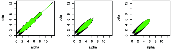
Figure 3: Plot of $(\alpha,\beta)$ corresponding to $\operatorname{Beta}(\alpha,\beta)$ priors that are weakly informative at level $\gamma=0.05$ (light and dark shading) and uniformly weakly informative (light shading) for $n=20$ (on the left), $n=100$ (middle) and $n=\infty$ (on the right).

We want to investigate the weak informativity of a $\operatorname{Gamma}_{\mathrm{rate}}(\alpha_{2},\beta_{2})$ prior relative to a $\operatorname{Gamma}_{\mathrm{rate}}(\alpha_{1},\break\beta_{1})$ prior. For finite $n$ this is a difficult problem, so we simplify this by considering only the asymptotic case. When the prior is $\Pi_{i}$, then, as $n\rightarrow\infty$, we have that $m_{iT,n}(t)\rightarrow m_{iT}(t)=(\beta_{i}^{\alpha_{i}}/\Gamma(\alpha_{i}))t^{-\alpha_{i}-1}e^{-\beta_{i}/t}$, that is, $1/t\sim\operatorname{Gamma}_{\mathrm{rate}}(\alpha_{i},\beta_{i})$ in the limit.Therefore, $P_{2,n}(t_{0})\rightarrow P_{2}(t_{0})=\Pi_{2}(t^{-\alpha_{2}-1/2}e^{-\beta_{2}/t}\leq\break t_{0}^{-\alpha_{2}-1/2}\cdot e^{-\beta_{2}/t_{0}})$ and we want to determine conditions on $(\alpha_{2},\beta_{2})$ so that $\Pi_{1}(P_{2}(t)\leq\gamma)\leq\gamma$.

While results can be obtained for this problem, it is still rather difficult. It is greatly simplified, however, if we impose a natural restriction on $(\alpha_{2},\beta_{2})$. In particular, we want the location of the bulk of the mass for $\Pi_{2}$ to be located roughly in the same place as the bulk of the mass for $\Pi_{1}$. Accordingly, we could require the priors to have the same means or modes, but, as it turns out, the constraint that requires the modes of the $m_{iT}^{\ast}$ functions to be the same greatly simplifies the analysis. Actually, $m_{iT,n}^{\ast}(t)$ converges to 0, but the $n$’s cancel in the inequalities defining $P_{i,n}(t_{0})$ and so we can define $m_{iT,n}^{\ast}(t)=\break t^{-\alpha_{i}-1/2}e^{-\beta_{i}/t}$ which has its mode at $t=\beta_{i}/(\alpha_{i}+1/2)$. Therefore, we must have $\beta_{2}/(\alpha_{2}+1/2)=\beta_{1}/\break(\alpha_{1}+1/2)$ so that $(\alpha_{2},\beta_{2})$ lies on the line through the points $(0,\beta_{1}/2(\alpha_{1}+1/2))$ and $(\alpha_{1},\beta_{1})$. We prove the following result in the Appendix.

Theorem 4.

Suppose we use a $\operatorname{Gamma}_{\mathrm{rate}}(\alpha_{1},\break\beta_{1})$ prior on $1/\sigma^{2}$ when sampling from the statistical model $\{N(0,\sigma^{2})\dvtx\sigma^{2}>0\}$. Then a $\operatorname{Gamma}_{\mathrm{rate}}(\alpha_{2},\beta_{2})$ prior on $1/\sigma^{2}$, with $\beta_{2}/(\alpha_{2}+1/2)=\beta_{1}/(\alpha_{1}+1/2)$, is asymptotically weakly informative relative to the $\operatorname{Gamma}_{\mathrm{rate}}(\alpha_{1},\beta_{1})$ prior whenever $\alpha_{2}\leq\alpha_{1}$ and $\beta_{2}=\beta_{1}(\alpha_{2}+1/2)/(\alpha_{1}+1/2)$ or, equivalently, whenever $\beta_{1}/2(\alpha_{1}+1/2)\leq\beta_{2}\leq\beta_{1}$ and $\alpha_{2}=(\alpha_{1}+1/2)\beta_{2}/\beta_{1}-1/2$.

Of particular interest here is that we cannot reduce the rate parameter $\beta_{2}$ arbitrarily close to 0 and be guaranteed asymptotic weak informativity.

4 Applications

We consider now some applications of determining weakly informative priors.

4.1 Weakly Informative Beta Priors for the Binomial

Suppose that $T\!\sim\!\operatorname{Binomial}(n,\theta)$ and $\theta\!\sim\!\operatorname{Beta}(\alpha,\beta)$. This implies that $m_{T}(t)=\bigl{(}{{n}\atop{t}}\bigr{)}\Gamma(\alpha+\beta)\Gamma(t+\alpha)\Gamma(n-t+\beta)/\Gamma(\alpha)\Gamma(\beta)\Gamma(n+\alpha+\beta)$ and from this we can compute (4) for various choices of $(\alpha,\beta)$.

As a specific example, suppose that $n=20$, the base prior is given by $(\alpha,\beta)=(6,6)$, and we take $\gamma=0.05$ so that $x_{0.05}=0.0588$. As alternatives to this base prior, we consider $\operatorname{Beta}(\alpha,\beta)$ priors. In Figure 3 we have plotted all the $(\alpha,\beta)$ corresponding to $\operatorname{Beta}(\alpha,\beta)$ distributions that are weakly informative with respect to the $\operatorname{Beta}(6,6)$ distribution at level $0.05$, together with the subset of all $(\alpha,\beta)$ corresponding to $\operatorname{Beta}(\alpha,\beta)$ distributions that are uniformly weakly informative relative to the $\operatorname{Beta}(6,6)$ distribution. The graph on the left corresponds to $n=20$, the middle graph corresponds to $n=100$, and the graph on the right corresponds to $n=\infty$. The plot for $n=20$ shows some anomalous effects due to the discreteness of the prior predictive distributions and these effects disappear as $n$ increases. In such an application we may choose to restrict to symmetric priors, as this fixes the primary location of the prior mass. For example, when $n=20$, a $\operatorname{Beta}(\alpha,\alpha)$ prior for $\alpha$ satisfying $1\leq\alpha\leq 12.3639$ is uniformly weakly informative with respect to the $\operatorname{Beta}(6,6)$ prior and we see that values of $\alpha>6$ are eliminated as $n$ increases.

4.2 Weakly Informative Priors for the Normal Regression Model

Consider the situation where $y\sim N_{n}(X\beta,\sigma^{2}I)$, $X\in R^{n\times k}$ is of rank $k$ and $\beta\in R^{k},\sigma^{2}>0$ are unknown. Therefore, $T=(b,s^{2})$ with $b=(X^{\prime}X)^{-1}X^{\prime}y$ and $s^{2}=\|y-Xb\|^{2}$. Suppose we have elicited a prior on $(\beta,\sigma^{2})$ given by $1/\sigma^{2}\sim\operatorname{Gamma}_{\mathrm{rate}}(\alpha_{1},\tau_{1})$, and $\beta|\sigma^{2}\sim N_{k}(\beta_{0},\sigma^{2}\Sigma_{1})$. We now find a prior that is asymptotically uniformly weakly informative relative to this choice. For this we consider gamma priors for $1/\sigma^{2}$ and $t$ priors for $\beta$ given $\sigma^{2}$. For the asymptotics we suppose that $\lambda_{k}((X^{\prime}X)^{-1})\rightarrow 0$ as $n\rightarrow\infty$.

As discussed in Evans and Moshonov (2006, 2007), it seems that the most sensible way to check for prior-data conflict here is to first check the prior on $\sigma^{2}$, based on the prior predictive distribution of $s^{2}$. If no prior-data conflict is found at this stage, then we check the prior on $\beta$ based on the conditional prior predictive for $b$ given $s^{2}$, as $s^{2}$ is ancillary for $\beta$. Such an approach provides more information concerning where a prior-data conflict exists than simply checking the whole prior via (3).

So we consider first obtaining an asymptotically uniformly weakly informative prior for $1/\sigma^{2}$. We have that $s^{2}|\sigma^{2}\sim\operatorname{Gamma}_{\mathrm{rate}}((n-k)/2,(n-k)/2\sigma^{2})$ and so, as in Section 3.3, when $1/\sigma^{2}\sim\operatorname{Gamma}_{\mathrm{rate}}(\alpha_{i},\break\tau_{i})$, the limiting prior predictive distribution of $1/s^{2}$ is $\operatorname{Gamma}_{\mathrm{rate}}(\alpha_{i},\tau_{i})$ as $n\rightarrow\infty$. Furthermore, when $T_{2}(x)=s^{2}$, then $J_{T_{2}}(x)=(4s^{2}/(n-k))^{-1/2}$. Therefore, the limiting value of (4) in this case is the same as that discussed in Section 3.3 and Theorem 4 applies to obtain a $\operatorname{Gamma}_{\mathrm{rate}}(\alpha_{2},\tau_{2})$ prior asymptotically uniformly weakly informative relative to the $\operatorname{Gamma}_{\mathrm{rate}}(\alpha_{1},\tau_{1})$ prior.

If we consider $s^{2}$ as an arbitrary fixed value from its prior predictive distribution, then, when $\beta|\sigma^{2}\sim N_{k}(\beta_{0},\sigma^{2}\Sigma_{1})$, the conditional prior predictive distribution of $b$ given $s^{2}$ converges to the $N_{k}(\beta_{0},s^{2}\Sigma_{1})$ distribution. Furthermore, when $\beta|\sigma^{2}\sim t_{k}(\beta_{0},\sigma^{2}\Sigma_{2},\break\lambda)$, the conditional prior predictive distribution of $b$ given $s^{2}$ converges to the $t_{k}(\beta_{0},s^{2}\Sigma_{2},\lambda)$ distribution. So we can apply Lemma 1 to these limiting distributions. It is then clear that the comparison is covered by Theorem 3, as the limiting prior predictives are of the same form. Therefore, the $t_{k}(\beta_{0},\sigma^{2}\Sigma_{2},\lambda)$ prior is asymptotically uniformly weakly informative relative to the $N_{k}(\beta_{0},\sigma^{2}\Sigma_{1})$ prior whenever $s^{2}\Sigma_{2}\geq s^{2}\tau_{\lambda}^{2}\Sigma_{1}$ or, equivalently, whenever $\Sigma_{2}\!\geq\!\tau_{\lambda}^{2}\Sigma_{1}$ where $\tau_{\lambda}^{2}$ is defined in Theorem 3. Note that this condition does not depend on $s^{2}$. Also, as $\lambda\rightarrow\infty$, we can use Theorem 2 to obtain that a $N_{k}(\beta_{0},\sigma^{2}\Sigma_{2})$ prior is asymptotically uniformly weakly informative relative to the $N_{k}(\beta_{0},\sigma^{2}\Sigma_{1})$ prior whenever $\Sigma_{2}\geq\Sigma_{1}$.

4.3 Weakly Informative Priors for Logistic Regression

Supposing we have a single binary valued response variable $Y$ and $k$ quantitative predictors $X_{1},\ldots,X_{k}$, we observe $(Y,X_{1},\ldots,X_{k})$ at $q$ settings of the predictor variables and have $n_{i}$ observations at the $i$th setting of the predictors. The logistic regression model then says that $Y_{ij}\sim\operatorname{Bernoulli}(p_{i})$ where $\log(p_{i}/\break(1-p_{i}))=\beta_{0}+\beta_{1}(x_{i1}-\bar{x}_{\cdot 1})+\cdots+\beta_{k}(x_{ik}-\bar{x}_{\cdot k})$ for $j=1,\ldots,n_{i}$ and $i=1,\ldots,q$ and the $\beta_{i}$ are unknown real values. For simplicity, we will assume no $x_{ij}-\bar{x}_{\cdot j}$ is zero. For this model $T=(T_{1},\ldots,T_{q})$, with $T_{i}=Y_{i1}+\cdots+Y_{in_{i}}$, is a minimal sufficient statistic. For the base prior we suppose that $\Pi_{1}$ is the product of independent priors on the $\beta_{i}$’s and we consider the problem of finding a prior $\Pi_{2}$ that is weakly informative relative to $\Pi_{1}$. For example, we could take $\Pi_{1}$ to be a product of $N(0,\sigma_{1i}^{2})$ priors and $\Pi_{2}$ to be a product of $N(0,\sigma_{2i}^{2})$ priors and choose the $\sigma_{2i}^{2}$ so that weak informativity is obtained. Note that since $T$ is discrete we can use (2) in our computations.

As we will see, it is not the case that choosing the $\sigma_{2i}^{2}$ very large relative to the $\sigma_{1i}^{2}$ will necessarily make $\Pi_{2}$ weakly informative relative to $\Pi_{1}$. In fact, there is only a finite range of $\sigma_{2i}^{2}$ values where weak informativity will obtain.

While this can be demonstrated analytically, the argument is somewhat technical and it is perhaps easier to see this in an example. The following bioassay data are from Racine et al. (1986) and were also analyzed in Gelman et al. (2008). These data arise from an experiment where 20 animals were exposed to four doses of a toxin and the number of deaths recorded (Table 1).

Table 1:

Dose (g$\bolds{/}$ml)	Number of animals $\bolds{n_{i}}$	Number of deaths $\bolds{t_{i}}$
0.422	5	0
0.744	5	1
0.948	5	3
2.069	5	5

Following Gelman et al. (2008), we took $X_{1}$ to be the variable formed by calculating the logarithm of dose and then standardizing to make the mean of $X_{1}$ equal to 0 and its standard deviation equal to 1$/$2. Gelman et al. (2008) placed independent Cauchy priors on the regression coefficients, namely, $\beta_{0}\sim t_{1}(0,10^{2},1)$ independent of $\beta_{1}\sim t_{1}(0,2.5^{2},1)$.

We consider four possible scenarios for the investigation of weak informativity at level $\gamma=0.05$ and uniform weak informativity. In Figure 4(a) we compare $\Pi_{2}=N(0,\sigma_{0}^{2})\times N(0,\sigma_{1}^{2})$ priors with the prior $\Pi_{1}=N(0,10^{2})\times N(0,2.5^{2})$. The entire region gives the $(\sigma_{0},\sigma_{1})$ values corresponding to priors that are weakly informative at level $\gamma=0.05$, while the lighter subregion gives the $(\sigma_{0},\sigma_{1})$ values corresponding to priors that are uniformly weakly informative. Note that some of the irregularity in the plots is caused by the fact that the prior predictive distributions of $T$ are discrete. The three remaining plots are similar where in Figure 4(b) $\Pi_{1}=t_{1}(0,10^{2},1)\times t_{1}(0,2.5^{2},1)$ and $\Pi_{2}=t_{1}(0,\sigma_{0}^{2},1)\times t_{1}(0,\sigma_{1}^{2},1)$, in Figure 4(c) $\Pi_{1}=N(0,10^{2})\times N(0,2.5^{2})$ and $\Pi_{2}=t_{1}(0,\break\sigma_{0}^{2},1)\times t_{1}(0,\sigma_{1}^{2},1)$, and in Figure 4(d) $\Pi_{1}=t_{1}(0,10^{2},\break 1)\times t_{1}(0,2.5^{2},1)$ and $\Pi_{2}=N(0,\sigma_{0}^{2})\times N(0,\sigma_{1}^{2})$. Note that these plots only depend on the data through the values of $X_{1}$.

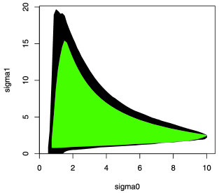
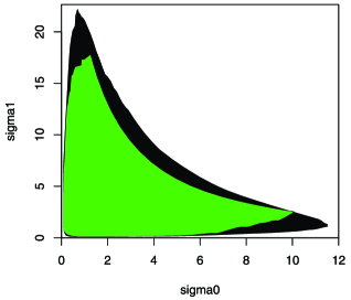
(a)	(b)
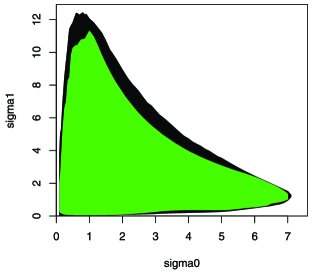
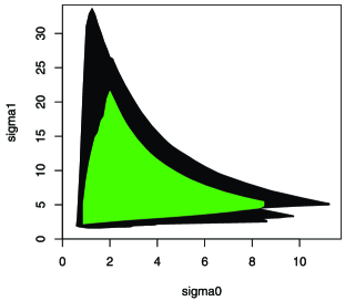
(c)	(d)

Figure 4: Weakly informative $\Pi_{2}$ priors relative to $\Pi_{1}$ at level 0.05 (light and dark shading) and uniformly weakly informative (light shading) where (a) $\Pi_{1}=N(0,10^{2})\times N(0,2.5^{2})$ and $\Pi_{2}=N(0,\sigma_{0}^{2})\times N(0,\sigma_{1}^{2})$, (b) $\Pi_{1}=t_{1}(0,10^{2},1)\times t_{1}(0,2.5^{2},1)$ and $\Pi_{2}=t_{1}(0,\sigma_{0}^{2},1)\times t_{1}(0,\sigma_{1}^{2},1)$, (c) $\Pi_{1}=N(0,10^{2})\times N(0,2.5^{2})$ and $\Pi_{2}=t_{1}(0,\sigma_{0}^{2},1)\times t_{1}(0,\sigma_{1}^{2},1)$ and (d) $\Pi_{1}=t_{1}(0,10^{2},1)\times\allowbreak t_{1}(0,2.5^{2},1)$ and $\Pi_{2}=N(0,\sigma_{0}^{2})\times N(0,\sigma_{1}^{2})$.

We see clearly from these plots that increasing the scaling on any of the $\beta_{i}$ does not necessarily lead to weak informativity and in fact inevitably destroys it. Furthermore, a smaller scaling on a parameter can lead to uniform weak informativity. These plots underscore how our intuition does not work very well with the logistic regression model, as it is not clear how priors on the $\beta_{i}$ ultimately translate to priors on the $p_{i}$. In fact, it can be proven that, if we put independent priors on the $\beta_{i}$, fix all the scalings but one, and let that scaling grow arbitrarily large, then the prior predictive distribution of $T$ converges to a distribution concentrated on two points, for example, when the scaling on $\beta_{0}$ increases these points are given by $\{\sum_{i=1}^{q}T_{i}=0\}\cup\{\sum_{i=1}^{q}T_{i}=\sum_{i=1}^{q}n_{i}\}$, and this is definitely not desirable. This partially explains the results obtained.

Of some interest is how much reduction we actually get, via (5), when we employ a weakly informative prior. In Figure 5 we have plotted contours of the choices of $(\sigma_{0},\sigma_{1})$ that give 0%, 25%, 50% and 75% reduction in prior-data conflicts for the case where $\Pi_{2}=N(0,\sigma_{0}^{2})\times N(0,\sigma_{1}^{2})$ and $\Pi_{1}=N(0,10^{2})\times N(0,2.5^{2})$ when $\gamma=0.05$ (this corresponds to $x_{\gamma}=0.0503$). Note that a substantial reduction can be obtained.

Figure 5: Reduction levels of $N(0,\sigma_{0}^{2})\times N(0,\sigma_{1}^{2})$ relative to $N(0,10^{2})\times N(0,2.5^{2})$ priors using (5) when $\gamma=0.05$. The plotted reduction levels are 0% (solid line), 25% (dashed line), 50% (dotted line) and 75% (long dashed line).

We can also consider fixing one of the scalings and seeing how much reduction we obtain when varying the other. For example, when we fix $\sigma_{0}=2.5$ we find that the maximum reduction is obtained when $\sigma_{1}$ is close to 2.2628, while if we fix $\sigma_{1}=2.5$, then the maximum reduction is obtained when $\sigma_{0}$ is close to 0.875.

It makes sense in any application to check to see if any prior-data conflict exists with respect to the base prior. If there is no prior-data conflict, this increases our confidence that the weakly informative prior is indeed putting less information into the analysis. This is assessed generally using (3), although (2) suffices in this example. When $\Pi_{1}=N(0,10^{2})\times N(0,2.5^{2})$, then (2) equals $0.1073$ and when $\Pi_{1}=t_{1}(0,10^{2},1)\times t_{1}(0,2.5^{2},1)$ (the prior used in Gelman et al., 2008), then (2) equals $0.1130$, so in neither case is there any evidence of prior-data conflict.

5 Refinements Based Upon Ancillarity

Consider an ancillary statistic that is a function of the minimal sufficient statistic, say, $U(T)$. The variation due to $U(T)$ is independent of $\theta$ and so should be removed from the $P$-value (3) when checking for prior-data conflict. Removing this variation is equivalent to conditioning on $U(T)$ and so we replace (3) by

$$M_{T}\bigl{(}m_{T}^{\ast}(t)\leq m_{T}^{\ast}(t_{0})|U(T)\bigr{)},$$ (9)

that is, we use the conditional prior predictive given the ancillary $U(T)$. To remove the maximal amount of ancillary variation, we must have that $U(T)$ is a maximal ancillary. Therefore, (4) becomes

$$M_{1T}\bigl{(}P_{2}(t_{0}|U(T))\leq x_{\gamma}|U(T)\bigr{)},$$ (10)

that is, we have replaced $P_{2}(t_{0})$ by $P_{2}(t_{0}|U(T))=M_{2T}(m_{2T}^{\ast}(t)\leq m_{2T}^{\ast}(t_{0})|U(T))$ and $M_{1T}$ by$M_{1T}(\cdot|U(T))$.

We note that the approach discussed in Section 2 works whenever $T$ is a complete minimal sufficient statistic. This is a consequence of Basu’s Theorem, as, in such a case, any ancillary is statistically independent of $T$ and so conditioning on such an ancillary is irrelevant. This is the case for the examples in Sections 3 and 4.

One problem with ancillaries is that multiple maximal ancillaries may exist. When ancillaries are used for frequentist inferences about $\theta$ via conditioning, this poses a problem because it is not clear which maximal ancillary to use and confidence regions depend on the maximal ancillary chosen. For checking for prior-data conflict via (9), however, this does not pose a problem. This is because we simply get different checks depending on which maximal ancillary we condition on. For example, if conditioning on maximal ancillary $U_{1}(T)$ does not lead to prior-data conflict, but conditioning on maximal ancillary $U_{2}(T)$ does, then we have evidence against no prior-data conflict existing.

Similarly, when we go to use (10), we can also simply look at the effect of each maximal ancillary on the analysis and make our assessment about $\Pi_{2}$ based on this. For example, we can use the maximum value of (10) over all maximal ancillaries to assess whether or not $\Pi_{2}$ is weakly informative relative to $\Pi_{1}$. When this maximum is small, we conclude that we have a small prior probability of finding evidence against the null hypothesis of no prior-data conflict when using $\Pi_{2}$. We illustrate this via an example.

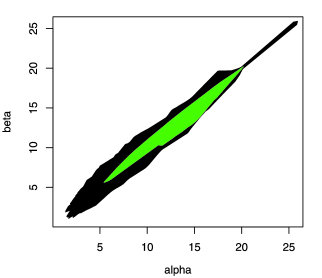
Figure 6: Plot of all $(\alpha,\beta)$ corresponding to $\operatorname{Beta}(\alpha,\beta)$ priors that are weakly informative at level $\gamma=0.05$ (light and dark shading) and uniformly weakly informative (light shading).

Example 1.

Suppose that we have a sample of $n$ from the $\operatorname{Multinomial}(1,(1-\theta)/6,(1+\theta)/6,(2-\theta)/6,(2+\theta)/6)$ distribution where $\theta\in[-1,1]$ is unknown. Then the counts $(f_{1},f_{2},f_{3},f_{4})$ constitute a minimal sufficient statistic and $U_{1}=(f_{1}+f_{2},f_{3}+f_{4})$ is ancillary, as is $U_{2}=(f_{1}+f_{4},f_{2}+f_{3})$. Then $T=(f_{1},f_{2},f_{3},f_{4})|U_{1}$ is given by $f_{1}|\ U_{1}\sim\ \mathrm{Binomial}(f_{1}+f_{2},(1-\theta)/2)$ independent of $f_{3}|\ U_{1}\sim\ \mathrm{Binomial}(f_{3}+f_{4},(2-\theta)/4)$, giving

$$m_{T}(f_{1},f_{2},f_{3},f_{4}|U_{1})$$

$$\quad=\pmatrix{{f_{1}+f_{2}}\cr{f_{1}}}{\pmatrix{f_{3}+f_{4}\cr{f_{3}}}}$$

$$\qquad\cdot\int_{-1}^{1}\biggl{(}\frac{1-\theta}{2}\biggr{)}^{f_{1}}\biggl{(}\frac{1+\theta}{2}\biggr{)}^{f_{2}}\biggl{(}\frac{2-\theta}{4}\biggr{)}^{f_{3}}$$

$$\qquad{}\cdot\biggl{(}\frac{2+\theta}{4}\biggr{)}^{f_{4}}\pi(\theta)\,d\theta.$$

We then have two 1-dimensional distributions $f_{1}|U_{1}$ and $f_{3}|U_{1}$ to use for checking for prior-data conflict. A similar result holds for the conditional distribution given $U_{2}$.

For example, suppose $\pi$ is a $\operatorname{Beta}(20,20)$ distribution on $[-1,1]$, so the prior concentrates about $0$, and for a sample of $n=18$ we have that $U_{1}=f_{1}+f_{2}=10$ and $U_{2}=f_{1}+f_{4}=8$. In Figure 6 we have plotted all the values of $(\alpha,\beta)$ that correspond to a $\operatorname{Beta}(\alpha,\beta)$ prior that is weakly informative relative to the $\operatorname{Beta}(20,20)$ prior at level $\gamma=0.05$, as well as those that are uniformly weakly informative. So for each such $(\alpha,\beta)$ we have that (10) is less than or equal to 0.05 for both $U=U_{1}$ and $U=U_{2}$.

6 Conclusions

We have developed an approach to measuring the amount of information a prior puts into a statistical analysis relative to another base prior. This base prior can be considered as the prior that best reflects current information and our goal is to determine a prior that is weakly informative with respect to it. Our measure is in terms of the prior predictive probability, using the base prior, of obtaining a prior-data conflict. This was applied in several examples where the approach is seen to give intuitively reasonable results. The examples chosen here focused on commonly used prior families. In several cases these were conjugate families, although there is no special advantage computationally to conjugacy in this context.

As noted in several examples, we need to be careful when we conceive of a prior being weakly informative relative to another. Ultimately this concept needs to be made precise and we feel our definition is a reasonable proposal. The definition has intuitive support, in terms of avoiding prior-data conflicts, and provides a quantifiable criterion that can be used to select priors.

In any application we should still check for prior-data conflict for the base prior using (3). If prior-data conflict is found, a substitute prior that is weakly informative relative to the base prior can then be selected and a check made for prior-data conflict with respect to the new prior. While selecting the prior based on the observed data is not ideal, this process at least seems defensible from a logical perspective. For example, the new prior still incorporates some of the information from the base prior and is not entirely driven by the data. Certainly, in the end it seems preferable to base an analysis on a prior for which a prior-data conflict does not exist. Of course, we must still report the original conflict and how this was resolved.

We have restricted our discussion here to proper priors. The concept of weak informativity is obviously related to the idea of noninformativity and improper priors. Certainly any prior that has a claim to being noninformative should not lead to prior-data conflict. At this time, however, there is no precise definition of what a noninformative prior is, whereas we have provided a definition of a weakly informative prior. In the examples of Section 3.1 and 3.2 we see that if the spread of $\Pi_{2}$ is made large enough, then $\Pi_{2}$ is uniformly weakly informative with respect to the base prior. This suggests that the flat improper prior, which is Jeffreys’ prior for this problem, can be thought of as always being uniformly weakly informative. The logistic regression example of Section 4.3 suggests caution, however, in interpreting increased diffuseness as a characterization of weak informativity. In the binomial example of Section 4.1 the uniform prior is always weakly informative with respect to the base prior, while the $\operatorname{Beta}(1/2,1/2)$ (Jeffreys’) prior is not. Further work is required for a full examination of the relationships among the concepts of prior-data conflict, noninformativity and weak informativity.

Appendix

Proof of Lemma 1 We have that $x_{\gamma}=\gamma$ since $P_{1}(t)$ has a continuous distribution under $M_{1T}$. Suppose $m_{iT}^{\ast}(t)$ has a point mass at $r_{0}$ when $t\sim M_{iT}$. The assumption $M_{iT}(m_{iT}^{\ast}(t)=r_{0})>0$ implies$(m_{iT}^{\ast})^{-1}\{r_{0}\}\not=\varnothing$. Then, pick $t_{r_{0}}\in(m_{iT}^{\ast})^{-1}\{r_{0}\}$ so that $m_{iT}^{\ast}(t_{r_{0}})=r_{0}$ and let $\eta_{i}=P_{i}(t_{r_{0}})$. Then, $P_{i}(t)$ has point mass at $\eta_{i}$ because $M_{iT}(P_{i}(t)=\eta_{i})\geq\break M_{iT}(m_{iT}^{\ast}(t)=m_{iT}^{\ast}(t_{r_{0}}))=M_{iT}(m_{iT}^{\ast}(t)=r_{0})>0$.This is a contradiction and so $m_{iT}^{\ast}(t)$ has a continuous distribution when $t\sim M_{iT}$.

Let $r_{\gamma}=\sup\{r\in\mathcal{R}\dvtx M_{2T}(m_{2T}^{\ast}(t)\leq r)\leq\gamma\}$ where $\mathcal{R}=\overline{\{m_{2T}^{\ast}(t)\dvtx t\in\mathcal{T}\}}$ and $\mathcal{T}$ is the range space of $T$. Then, $M_{2T}(m_{2T}^{\ast}(t)\leq r_{\gamma})=\gamma$ and $M_{2T}(m_{2T}^{*}(t)\leq\break r_{\gamma}+\epsilon)>\gamma$ for all $\epsilon>0$. Thus, we have that $\{t\dvtx\break P_{2}(t)\leq\gamma\}=\{t\dvtx m_{2T}^{\ast}(t)\leq r_{\gamma}\}$, $M_{1T}(P_{2}(t)\leq\gamma)=\break M_{1T}(m_{2T}^{\ast}(t)\leq r_{\gamma})$, and $\Pi_{2}$ is weakly informative at level $\gamma$ relative to $\Pi_{1}$ if and only if $M_{1T}(m_{2T}^{\ast}(t)\leq r_{\gamma})\leq\gamma$. The fact that $\{r_{\gamma}\dvtx\gamma\in[0,1]\}\subset\mathcal{R}$ implies the last statement.

Proof of Theorem 1 Suppose first that $\Sigma_{1}\leq\Sigma_{2}$. We have that $n^{-1}I+\Sigma_{1}\leq n^{-1}I+\Sigma_{2}$ and so $(n^{-1}I+\Sigma_{1})^{-1}\geq(n^{-1}I+\Sigma_{2})^{-1}$. This implies that (3.1) is less than $\gamma$ and so the $N_{k}(\mu_{0},\Sigma_{2})$ prior is uniformly weakly informative relative to the $N_{k}(\mu_{0},\Sigma_{1})$ prior.

For the converse put $V_{i}=\{y\dvtx y^{\prime}(n^{-1}I+\Sigma_{i})^{-1}y\leq 1\}$. If $V_{1}\subset V_{2}$, then for $y\in R^{k}\backslash\{0\}$ there exists $c>0$ such that $c^{2}y^{\prime}(n^{-1}I+\Sigma_{1})^{-1}y=1$ which implies $cy\in V_{2}$ and so $c^{2}y^{\prime}(n^{-1}I+\Sigma_{2})^{-1}y\leq 1$. This implies that $y^{\prime}(n^{-1}I+\Sigma_{1})^{-1}y\geq y^{\prime}(n^{-1}I+\Sigma_{2})^{-1}y$ and so $\Sigma_{1}\leq\Sigma_{2}$ and the result follows. If $V_{2}\subset V_{1}$, then the same reasoning says that $\Sigma_{2}\leq\Sigma_{1}$ and (3.1) would be greater than $\gamma$ if $\Sigma_{2}<\Sigma_{1}$.

So we need only consider the case where $V_{1}\cap V_{2}^{c}$, $V_{1}^{c}\cap V_{2}$ both have positive volumes, that is, we are supposing that neither $\Sigma_{2}-\Sigma_{1}$ nor $\Sigma_{1}-\Sigma_{2}$ is positive semidefinite and then will obtain a contradiction. Let $\delta=\inf\{y^{\prime}(n^{-1}I+\Sigma_{1})^{-1}y\dvtx y\in V_{1}\cap\partial V_{2}\}$ and note that $\delta<1$, since $V_{1}^{o}\cap\partial V_{2}\neq\phi$, that is, there are points in the interior of $V_{1}$ on the boundary of $V_{2}$. Now put $V_{0}=\{y\in V_{1}\cap V_{2}^{c}\dvtx y^{\prime}(n^{-1}I+\Sigma_{1})^{-1}y\leq(1+\delta)/2\}$ and note that $V_{0}$ has positive volume.

Let $Y\sim N_{k}(0,n^{-1}I+\Sigma_{1})$ and $\tau_{\gamma}^{2}=G_{k}^{-1}(1-\gamma)$. Then $M_{1T}(P_{1}(t)\,{\leq}\,\gamma\vspace*{1pt})\,{=}\,P(Y^{\prime}(n^{-1}I+\Sigma_{1})^{-1}Y\,{\geq}\,\tau_{\gamma}^{2})=P(Y\notin\tau_{\gamma}V_{1})=1-P_{Y}(\tau_{\gamma}(V_{1}\cap V_{2})\cup\tau_{\gamma}(V_{1}\cap V_{2}^{c}))$ while $M_{1T}(P_{2}(t)\leq\gamma)=P(Y^{\prime}(n^{-1}I+\Sigma_{2})^{-1}\cdot Y\geq\vspace*{1pt}\tau_{\gamma}^{2})=P(Y\notin\tau_{\gamma}V_{2})=1-P_{Y}(\tau_{\gamma}(V_{1}\cap V_{2})\cup\tau_{\gamma}(V_{1}^{c}\cap V_{2}))$. Since $\gamma=M_{1T}(P_{1}(t)\leq\gamma)$, we need only show that $P_{Y}(\tau_{\gamma}(V_{1}\cap V_{2}^{c}))>P_{Y}(\tau_{\gamma}(V_{1}^{c}\cap V_{2}))$ for all $\gamma$ sufficiently small, to establish the result.

Let $f(x)=k_{1}e^{-x/2}$ be such that $f(y^{\prime}(n^{-1}I+\break\Sigma_{1})^{-1}y)$ is the density of $Y$. Then $P_{Y}(\tau_{\gamma}(V_{1}^{c}\cap V_{2}))=\vspace*{1pt}\int_{\tau_{\gamma}(V_{1}^{c}\cap V_{2})}f(y^{\prime}(n^{-1}I+\Sigma_{1})^{-1}y)\,dy\leq f(\tau_{\gamma}^{2}y_{\ast}^{\prime}(n^{-1}I+\Sigma_{1})^{-1}y_{\ast})\operatorname{Vol}((V_{1}^{c}\cap V_{2}))\tau_{\gamma}^{k}$ where $y_{\ast}=\arg\min\{y^{\prime}\cdot(n^{-1}I+\Sigma_{1})^{-1}y\dvtx y\in V_{1}^{c}\cap V_{2}\}$. Note it is clear that $y_{\ast}\in\partial V_{1}$ and so $y_{\ast}^{\prime}(n^{-1}I+\Sigma_{1})^{-1}y_{\ast}=1$ and $f(\tau_{\gamma}^{2}y_{\ast}^{\prime}\cdot(n^{-1}I+\Sigma_{1})^{-1}y_{\ast})=k_{1}e^{-\tau_{\gamma}^{2}/2}$. Also, $P_{Y}(\tau_{\gamma}(V_{1}\cap V_{2}^{c}))\geq P_{Y}(\tau_{\gamma}V_{0})=\int_{\tau_{\gamma}V_{0}}f(y^{\prime}(n^{-1}I+\Sigma_{1})^{-1}y)\,dy\geq f(\tau_{\gamma}^{2}(1+\delta)/2)\operatorname{Vol}(V_{0})\tau_{\gamma}^{k}$ where $f(\tau_{\gamma}^{2}(1+\delta)/2)=k_{1}e^{-\tau_{\gamma}^{2}(1\vspace*{1pt}+\delta)/4}$. Therefore, as $\gamma\rightarrow 0$,

$$\frac{P_{Y}(\tau_{\gamma}(V_{1}\cap V_{2}^{c}))}{P_{Y}(\tau_{\gamma}(V_{1}^{c}\cap V_{2}))}$$

$$\quad\geq e^{\tau_{\gamma}^{2}(1-\delta)/4}\frac{\operatorname{Vol}((V_{1}^{c}\cap V_{2}))}{\operatorname{Vol}(V_{0})}\rightarrow\infty,$$

since $\tau_{\gamma}=(G_{k}^{-1}(1-\gamma))^{1/2}\rightarrow\infty$ as $\gamma\rightarrow 0$ and $0<\delta<1$.

Proof of Theorem 2 First note that we can use (2) instead of (3) in this case as $J_{T}(x)$ is constant in this case. We assume without loss of generality that $\mu_{0}=0.$

We first establish several useful technical results. If $\Pi_{i}$ is a probability distribution that is unimodal and symmetric about 0, and $\phi_{\nu}$ denotes a $N(0,\nu)$ density, we have that $m_{iT}(t)=\int_{R}\phi_{\nu}(t-\mu)\Pi_{i}(d\mu)$ is unimodal and symmetric about 0. We have the following result.

Lemma .1.

If $T$ is a minimal sufficient statistic, $J_{T}(x)$ is constant in $x$, $\Pi_{1}$ and $\Pi_{2}$ are unimodal and symmetric about 0, the $P_{i}(t)$ have continuous distributions when $t\sim M_{iT},m_{1T}(0)>m_{2T}(0)$, and $m_{1T}(t)=m_{2T}(t)$ has a unique solution for $t>0$$,\$then $\Pi_{2}$ is uniformly weakly informative relative to $\Pi_{1}$.

By the unimodality and symmetryof $m_{iT}$, we must have that $P_{i}(t)=M_{iT}(m_{iT}(u)\leq m_{iT}(t))=M_{iT}(|u|\geq|t|)$. We show $M_{1T}(|t|\geq t_{0})\leq M_{2T}(|t|\geq t_{0})$ for all $t_{0}>0$ because it is equivalent to $\Pi_{2}$ being uniformly weakly informative relative to $\Pi_{1}$ by Lemma 1. Let $t_{s}$ be the solution of $m_{1T}(t)=m_{2T}(t)$ on $(0,\infty)$. From the unique solution assumption, $m_{1T}(t)>m_{2T}(t)$ for $t\in(0,t_{s})$ and $m_{1T}(t)<m_{2T}(t)$ for $t>t_{s}$. For $0\leq t_{0}<t_{s},M_{1T}(|t|\geq t_{0})=2\int_{t_{0}}^{\infty}m_{1T}(t)\,dt=1-2\int_{0}^{t_{0}}m_{1T}(t)\,dt\leq 1-\break 2\int_{0}^{t_{0}}m_{2T}(t)\,dt=2\int_{t_{0}}^{\infty}m_{2T}(t)\,dt=M_{2T}(|t|\geq t_{0})$ and for $t_{0}\geq t_{s}$, $M_{1T}(|t|\geq t_{0})=2\int_{t_{0}}^{\infty}m_{1T}(t)\,dt\leq\break 2\int_{t_{0}}^{\infty}m_{2T}(t)\,dt,{=}\,M_{2T}(|t|\,{\geq}\,t_{0})$. Thus, we are done.

We can apply Lemma .1 to comparing normal and $t$ priors when sampling from a normal.

Lemma .2.

Suppose we have a sample of $n$ from a location normal model, $\Pi_{1}$ is a $N(0,\sigma_{1}^{2})$ prior and $\Pi_{2}$ is a $t_{1}(0,\sigma_{2}^{2},\lambda)$ prior. If $m_{1T}(0)>m_{2T}(0)$, then $\Pi_{2}$ is uniformly weakly informative relative to $\Pi_{1}$.

We have that $m_{1T}=\phi_{1/n+\sigma_{1}^{2}}$ and, using the representation of the $t(\lambda)$ distribution as a gamma mixture of normals, we write $m_{2T}(t)=\int_{0}^{\infty}\phi_{1/n+\sigma_{2}^{2}/u}(t)k_{\lambda}(u)\,du$ where $k_{\lambda}$ is the density of $\operatorname{Gamma}_{\mathrm{rate}}(\lambda/2,\lambda/2)$ distribution. By the symmetry of $\phi_{v}$, $m_{2T}$ is symmetric. Also, $\phi_{v}(t_{1})>\phi_{v}(t_{2})$ for $0\,{\leq}\,t_{1}\,{<}\,t_{2}$ and so $m_{2T}(t_{1})\,{=}\,\int\!\phi_{1/n+\sigma_{2}^{2}/u}(t_{1})k_{\lambda}(u)\,du\geq\int\phi_{1/n+\sigma_{2}^{2}/u}(t_{2})k_{\lambda}(u)\,du=m_{2T}(t_{2})$. Thus, $m_{2T}$ is decreasing on $(0,\infty)$, that is, $m_{2T}$ is unimodal. To show that $m_{2T}(t)$ is log-convex with respect to $t^{2}$, we prove that $(d^{2}/d(t^{2})^{2})\log m_{2T}(t)\geq 0$. Note that $(d/d(t^{2}))\phi_{v}(t)=(d/d(t^{2}))[(2\pi v)^{-1/2}\exp\{-t^{2}/2v\}]=-\phi_{v}(t)/2v$,

$$\frac{dm_{2T}(t)}{dt^{2}}$$

$$\quad=-\int_{0}^{\infty}\frac{\phi_{1/n+\sigma_{2}^{2}/u}(t)}{2(1/n+\sigma_{2}^{2}/u)}k_{\lambda}(u)\,du,$$

$$\frac{d^{2}\log m_{2T}(t)}{d(t^{2})^{2}}$$

$$\quad=\frac{1}{m_{2T}(t)}\int_{0}^{\infty}\frac{\phi_{1/n+\sigma_{2}^{2}/u}(t)}{[2(1/n+\sigma_{2}^{2}/u)]^{2}}k_{\lambda}(u)\,du$$

$$\qquad{}-\frac{1}{m_{2T}(t)^{2}}\biggl{(}\int_{0}^{\infty}\frac{\phi_{1/n+\sigma_{2}^{2}/u}(t)}{2(1/n+\sigma_{2}^{2}/u)}k_{\lambda}(u)\,du\biggr{)}^{2}$$

and so $d^{2}\log m_{2T}(t)/d(t^{2})^{2}=\operatorname{Var}_{V}([2(1/n+\break\sigma_{2}^{2}/V)]^{-1})\geq 0$, where $V$ is the random variable having density $\phi_{1/n+\sigma_{2}^{2}/v}(t)k_{\lambda}(v)/m_{2T}(t)$. Thus, $m_{2T}(t)$ is log-convex in $t^{2}$.

The functions $m_{1T}(t)$ and $m_{2T}(t)$ meet in at most two points on $(0,\infty)$ because $\log m_{1T}(t)$ is linear in $t^{2}$ and $\log m_{2T}(t)$ is convex in $t^{2}$. Also, $m_{1T}(t)$ and $m_{2T}(t)$ share at least one point on $(0,\infty)$ because $m_{1T}(0)>m_{2T}(0)$, and the following shows that $m_{1T}(t)<m_{2T}(t)$ for all large $t$. Note first that if $u\geq\sigma_{2}^{2}/2\sigma_{1}^{2}$, then $(1/n+\sigma_{1}^{2})/(1/n+\sigma_{2}^{2}/u)\geq 1/2$ and $t^{2}/(u/n+\sigma_{2}^{2})\geq(2\sigma_{1}^{2}/\sigma_{2}^{2})t^{2}/(1/n+2\sigma_{1}^{2})$. Then,

$$\frac{m_{2T}(t)}{m_{1T}(t)}$$

$$\quad\geq\int_{\sigma_{2}^{2}/2\sigma_{1}^{2}}^{\infty}\frac{(\lambda/2)^{\lambda/2}}{\Gamma(\lambda/2)}\frac{(2\pi(1/n+\sigma_{2}^{2}/u))^{-1/2}}{(2\pi(1/n+\sigma_{1}^{2}))^{-1/2}}u^{\lambda/2-1}$$

$$\hskip 32.0pt\qquad{}\cdot\frac{\exp\{-(u/2)(\lambda+t^{2}/({u/n+\sigma_{2}^{2}}))\}}{\exp\{-(1/2)t^{2}/(1/n+\sigma_{1}^{2})\}}\,du$$

$$\quad\geq\frac{(\lambda/2)^{\lambda/2}}{\Gamma(\lambda/2)}\frac{1}{2^{1/2}}\biggl{(}\frac{\sigma_{2}^{2}}{2\sigma_{1}^{2}}\biggr{)}^{\lambda/2-1}$$

$$\qquad{}\cdot\int_{\sigma_{2}^{2}/2\sigma_{1}^{2}}^{\infty}{\exp\biggl{\{}-\biggl{(}\frac{u}{2}\biggr{)}\biggl{(}\lambda+\frac{(2\sigma_{1}^{2}/\sigma_{2}^{2})t^{2}}{1/n+2\sigma_{1}^{2}}\biggr{)}\biggr{\}}}$$

$$\hskip 38.0pt\qquad{}\cdot\biggl{(}\exp\biggl{\{}\frac{-(1/2)t^{2}}{(1/n+\sigma_{1}^{2})}\biggr{\}}\biggr{)}^{-1}\,du$$

$$\quad=\frac{(\lambda/2)^{\lambda/2}}{\Gamma(\lambda/2)}\frac{1}{2^{1/2}}$$

$$\qquad{}\cdot\biggl{(}\frac{\sigma_{2}^{2}}{2\sigma_{1}^{2}}\biggr{)}^{\lambda/2-1}\exp\{-(1/2)(\sigma_{2}^{2}/2\sigma_{1}^{2})\lambda\}$$

$$\qquad{}\cdot{\exp\biggl{\{}\!\biggl{(}\frac{1}{2}\biggr{)}t^{2}\biggl{(}\!\biggl{(}\frac{1}{n}+\sigma_{1}^{2}\biggr{)}^{-1}-\biggl{(}\frac{1}{n}+2\sigma_{1}^{2}\biggr{)}^{-1}\biggr{)}\!\biggr{\}}}$$

$$\qquad{}\cdot\biggl{\{}2^{-1}\biggl{(}\lambda+\frac{(2\sigma_{1}^{2}/\sigma_{2}^{2})t^{2}}{(1/n+2\sigma_{1}^{2})}\biggr{)}\biggr{\}}^{-1}\rightarrow\infty$$

as $t^{2}\rightarrow\infty$.

The above conditions together imply that $m_{1T}(t)$ and $m_{2T}(t)$ meet in exactly one point on $(0,\infty)$. Therefore, $\Pi_{2}$ is uniformly weakly informative relative to $\Pi_{1}$ by Lemma .1.

Since $\int_{0}^{\infty}(1/n+\sigma^{2}/u)^{-1/2}k_{\lambda}(u)\,du$ is strictly decreasing in $\sigma^{2}$, we see that $m_{1T}(0)=(2\pi(1/n+\break\sigma_{1}^{2}))^{-1/2}\geq m_{2T}(0)=(2\pi)^{-1/2}\int_{0}^{\infty}(1/n+\sigma_{2}^{2}/u)^{-1/2}\cdot k_{\lambda}(u)\,du$ is equivalent to $\sigma_{2}\geq\sigma_{0n}$ where $\sigma_{0n}$ satisfies $(1/n+\sigma_{1}^{2})^{-1/2}=\int_{0}^{\infty}(1/n+\sigma_{0n}^{2}/u)^{-1/2}k_{\lambda}(u)\,du$. This proves the first part of Theorem 2.

We also need the following results for the remaining parts of Theorem 2.

Lemma .3.

(i) $\sigma_{0n}^{2}/\sigma_{1}^{2}$ increases as $n\sigma_{1}^{2}\rightarrow\infty$, (ii) $\sigma_{0n}^{2}/\sigma_{1}^{2}\rightarrow(2/\lambda)\Gamma^{2}((\lambda+1)/2)/\Gamma^{2}(\lambda/2)$ as$n\sigma_{1}^{2}\rightarrow\infty$.

(i) We have $n^{-1/2}(1/n+\sigma_{1}^{2})^{-1/2}=\break n^{-1/2}\int_{0}^{\infty}(1/n+\sigma_{0n}^{2}/u)^{-1/2}k_{\lambda}(u)\,du$ and putting $\alpha=n\sigma_{1}^{2},\beta=n\sigma_{0n}^{2}$, we can write this as

$$\qquad(1+\alpha)^{-1/2}=\int_{0}^{\infty}(1+\beta/u)^{-1/2}k_{\lambda}(u)\,du.$$ (1)

Differentiating both sides of (1) with respect to $\alpha$, we have $(1+\alpha)^{-3/2}=\int_{0}^{\infty}(1+\beta/\break u)^{-3/2}u^{-1}k_{\lambda}(u)\,du(d\beta/d\alpha)$. If we let $U\sim\break\operatorname{Gamma}_{\mathrm{rate}}(\lambda/2,\lambda/2)$, then this integral can be written as the expectation

$$E\bigl{(}(1+\beta/U)^{-3/2}U^{-1}\bigr{)}$$

$$\quad=E\bigl{(}(1+\beta/U)^{-3/2}(\beta/U+1-1)/\beta\bigr{)}$$

$$\quad=\beta^{-1}E\bigl{(}(1+\beta/U)^{-1/2}\bigr{)}$$

$$\qquad{}-\beta^{-1}E\bigl{(}(1+\beta/U)^{-3/2}\bigr{)}$$

$$\quad\leq\beta^{-1}E\bigl{(}(1+\beta/U)^{-1/2}\bigr{)}$$

$$\qquad{}-\beta^{-1}\bigl{\{}E\bigl{(}(1+\beta/U)^{-1/2}\bigr{)}\bigr{\}}^{3}$$

$$\quad=\beta^{-1}(1+\alpha)^{-1/2}-\beta^{-1}(1+\alpha)^{-3/2}$$

$$\quad=(1+\alpha)^{-3/2}(\alpha/\beta),$$

where the inequality follows via Jensen’s inequality. Hence, $d\beta/d\alpha=(1+\alpha)^{-3/2}[E((1+\beta/U)^{-3/2}\cdot U^{-1})]^{-1}\geq\beta/\alpha$ and so $\beta/\alpha$ is an increasing function of $\alpha$ because $d(\beta/\alpha)/d\alpha=\alpha^{-1}(d\beta/d\alpha)-\beta/\alpha^{2}\geq 0$. This proves $\sigma_{0n}^{2}/\sigma_{1}^{2}=n\sigma_{0n}^{2}/n\sigma_{1}^{2}=\beta/\alpha$ increases as $\alpha=n\sigma_{1}^{2}\rightarrow\infty$.

(ii) It is easy to check that $\beta=0$ when $\alpha=0$ and $\beta>0$ for $\alpha>0$. Let $\alpha_{0},\beta_{0}$ be a pair satisfying $\alpha_{0}>0$ and (1). Then, $\beta/\alpha\geq\beta_{0}/\alpha_{0}>0$ for $\alpha>\alpha_{0}$ and $\beta\rightarrow\infty$ as $\alpha\rightarrow\infty$. Therefore,

$$\lim_{\alpha\rightarrow\infty}\biggl{(}\frac{\beta}{\alpha}\biggr{)}^{1/2} = \lim_{\alpha\rightarrow\infty}\frac{\sqrt{\beta}}{\sqrt{1+\alpha}}$$

$$= \lim_{\alpha\rightarrow\infty}E\biggl{(}\frac{\sqrt{\beta}}{\sqrt{1+\beta/U}}\biggr{)}$$

$$= \lim_{\beta\rightarrow\infty}E\biggl{(}\frac{\sqrt{\beta}}{\sqrt{1+\beta/U}}\biggr{)}=E\bigl{(}\sqrt{U}\bigr{)}$$

$$= \int_{0}^{\infty}\sqrt{u}k_{\lambda}(u)\,du$$

$$= (2/\lambda)^{1/2}\Gamma\bigl{(}(\lambda+1)/2\bigr{)}/\Gamma(\lambda/2)$$

and this proves (ii).

Lemma .4.

Suppose we have a sample of $n$ from a location normal model, $\Pi_{1}$ is a $N(0,\sigma_{1}^{2})$ prior and $\Pi_{2}$ is a $t_{1}(0,\sigma_{2}^{2},\lambda)$ prior. Then $\Pi_{2}$ is asymptotically uniformly weakly informative relative to $\Pi_{1}$ if and only if $\sigma_{2}^{2}/\sigma_{1}^{2}\geq(2/\lambda)\Gamma^{2}((\lambda+1)/2)/\Gamma^{2}(\lambda/2)$.

Suppose that $\sigma_{2}^{2}/\sigma_{1}^{2}\geq(2/\lambda)\Gamma^{2}((\lambda+1)/\break 2)/\Gamma^{2}(\lambda/2)$. Then by Lemma .3 $\sigma_{2}^{2}/\sigma_{1}^{2}\geq\sigma_{0n}^{2}/\sigma_{1}^{2}$ for all $n$ and so $\Pi_{2}$ is uniformly weakly informative with respect to $\Pi_{1}$ for all $n$. So (4) is bounded above by $\gamma$ for all $n$ and so the limiting value of (4) is also bounded above by $\gamma$. This establishes that $\Pi_{2}$ is asymptotically uniformly weakly informative relative to $\Pi_{1}$.

Suppose now that $\sigma_{2}^{2}/\sigma_{1}^{2}<(2/\lambda)\Gamma^{2}((\lambda+1)/2)/\break\Gamma^{2}(\lambda/2)$. Note that $m_{1T}(t)=\lim_{n\rightarrow\infty}m_{1T,n}(t)=\break(2\pi\sigma_{1}^{2})^{-1/2}\exp(-t^{2}/(2\sigma_{1}^{2}))$ and $m_{2T}(t)=\break\lim_{n\rightarrow\infty}m_{2T,n}(t)=\Gamma((\lambda+1)/2)/(\Gamma(\lambda/2)\sqrt{\pi\lambda\sigma_{2}^{2}})(1+x^{2}/(\sigma_{2}^{2}\lambda))^{-(\lambda+1)/2}$. Therefore, we get $m_{1T}(0)=\break 1/\sqrt{2\pi\sigma_{1}^{2}}<\Gamma((\lambda+1)/2)/\Gamma(\lambda/2)\sqrt{\pi\lambda\sigma_{2}^{2}}=m_{2T}(0)$. Let $B=\{t\dvtx m_{2T}(t)>m_{1T}(0)\}$ and $\gamma=M_{2T}(B^{c})$. Then, $m_{1T}(t)\leq m_{1T}(0)\leq m_{2T}(t)$ on $B$ and$M_{1T}(P_{2}(t)\leq\gamma)=M_{1T}(B^{c})=1-M_{1T}(B)=1-\break\int_{B}m_{1T}(t)\,dt\geq 1-\int_{B}m_{1T}(0)\,dt\geq 1-\int_{B}m_{2T}(t)\,dt=M_{2T}(B^{c})=\gamma$. Hence, $\Pi_{2}$ is not weakly informative relative to $\Pi_{1}$ at level $\gamma$. Therefore, $\sigma_{2}^{2}/\sigma_{1}^{2}\geq(2/\break\lambda)\Gamma^{2}((\lambda+1)/2)/\Gamma^{2}(\lambda/2)$.

It is now immediate that $\sup_{\gamma\in[0,1]}G_{1}^{-1}(1-\gamma)/\break H_{1,\lambda}^{-1}(1-\gamma)=(2/\lambda)\Gamma^{2}((\lambda+1)/2)/\Gamma^{2}(\lambda/2)$ and the proof of Theorem 2 is complete.

Proof of Theorem 3 Since the minimal sufficient statistic $T(x)=\bar{x}$ is linear, there is no volume distortion and we can use (2) instead of (3). The limiting prior predictive distribution of $T(x)=\bar{x}$ under $\Pi_{1}$ is $N(\mu_{0},\Sigma_{1})$ and under $\Pi_{2}\$it is $t_{k}(\mu_{0},\Sigma_{2},\lambda)$. It is easy to check that $U_{1}=(T-\mu_{0})^{\prime}\Sigma_{1}^{-1}(T-\mu_{0})\sim\chi^{2}(k)$ when $T\sim\Pi_{1}$ and $U_{2}=(T-\mu_{0})^{\prime}\Sigma_{2}^{-1}(T-\mu_{0})\sim kF_{k,\lambda}$ when $T\sim\Pi_{2}$. This implies that $P_{2,n}(t_{0})$ converges to $P_{2}(t_{0})=\Pi_{2}(\pi_{2}(t)\leq\pi_{2}(t_{0}))=1-H_{k,\lambda}((t_{0}-\mu_{0})^{\prime}\Sigma_{2}^{-1}(t_{0}-\mu_{0})/k)$, where $H_{k,\lambda}$ is the distribution function of an $F_{k,\lambda}$ distribution. Further, we have that (4) converges to $\Pi_{1}(P_{2}(t)\leq\gamma)$.

Let $V_{i}=\{u\in R^{k}\dvtx u^{\prime}\Sigma_{i}^{-1}u<1\}$ for $i=1,2$. By the continuity of $\Pi_{2}(\pi_{2}(t)\leq r)$ as a function of $r$, and the continuity of $\pi_{2}(t)$, there exists $t_{0}$ such that $P_{2}(t)\leq\gamma$ if and only if $\pi_{2}(t)\leq\pi_{2}(t_{0})$. Hence, $\Pi_{2}$ is asymptotically uniformly weakly informative relative to $\Pi_{1}$ if and only if $\Pi_{1}(\pi_{2}(t)\leq\pi_{2}(t_{0}))\leq\break\Pi_{2}(\pi_{2}(t)\leq\pi_{2}(t_{0}))$ for all $t_{0}\in R^{k}$ by Lemma 1. Since $\pi_{2}(t)$ is decreasing in $u_{2}=U_{2}(t)$, the set $\{\pi_{2}(t)\leq\pi_{2}(t_{0})\}=\{u_{2}(t)\geq u_{2}(t_{0})\}=\mu_{0}+u_{2}(t_{0})V_{2}^{c}$. So we must prove that $\Pi_{1}(\mu_{0}+r^{1/2}V_{2}^{c})\leq\Pi_{2}(\mu_{0}+r^{1/2}V_{2}^{c})$ for all $r\geq 0$.

The positive semidefiniteness of $\Sigma_{2}-\tau_{\lambda}^{2}\Sigma_{1}$ implies that $\Sigma_{1}^{-1}/\tau_{\lambda}^{2}-\Sigma_{2}^{-1}$ is positive semidefinite. Then, for $u\in V_{2}^{c}$, that is, $u^{\prime}\Sigma_{2}^{-1}u\geq 1$, we have $u^{\prime}\Sigma_{1}^{-1}u=\tau_{\lambda}^{2}\cdot u^{\prime}(\Sigma_{1}^{-1}/\tau_{\lambda}^{2})u\geq\tau_{\lambda}^{2}u^{\prime}\Sigma_{2}^{-1}u\geq\tau_{\lambda}^{2}$. Thus, $V_{2}^{c}\subset\tau_{\lambda}V_{1}^{c}$.

Now we prove a stronger inequality $\Pi_{1}(\mu_{0}+\break r^{1/2}\tau_{\lambda}\cdot V_{1}^{c})\leq\Pi_{2}(\mu_{0}+r^{1/2}V_{2}^{c})$ for all $r\geq 0$. Note that

$$\Pi_{1}(\mu_{0}+r^{1/2}\tau_{\lambda}V_{1}^{c})$$

$$\quad=\Pi_{1}\bigl{(}u_{1}(t)\geq r\tau_{\lambda}^{2}\bigr{)}$$

$$\quad=\int_{r\tau_{\lambda}^{2}}^{\infty}\frac{2^{-k/2}}{\Gamma(k/2)}u^{k/2-1}e^{-u/2}\,du,$$

$$\Pi_{2}(\mu_{0}+r^{1/2}V_{2}^{c})$$

$$\quad=\Pi_{2}(u_{2}(t)\geq r)$$

$$\quad=\int_{r/k}^{\infty}\frac{\Gamma((k+\lambda)/2)}{\Gamma(k/2)\Gamma(\lambda/2)}$$

$$\qquad{}\cdot\biggl{(}\frac{k}{\lambda}\biggr{)}^{k/2}u^{k/2-1}\biggl{(}1+\frac{ku}{\lambda}\biggr{)}^{-(k+\lambda)/2}\,du,$$

and set $f(r)=\Pi_{2}(\mu_{0}+r^{1/2}V_{2}^{c})-\Pi_{1}(\mu_{0}+r^{1/2}\tau_{\lambda}\cdot V_{1}^{c})$. Then, $f(0)=0$ and

$$\frac{df(r)}{dr} = \frac{2^{-k/2}}{\Gamma(k/2)}(r\tau_{\lambda}^{2})^{k/2-1}e^{-r\tau_{\lambda}^{2}/2}\tau_{\lambda}^{2}$$

$${}\cdot\frac{\Gamma((k+\lambda)/2)}{\Gamma(k/2)\Gamma(\lambda/2)}\biggl{(}\frac{k}{\lambda}\biggr{)}^{k/2}\biggl{(}\frac{r}{k}\biggr{)}^{k/2-1}$$

$${}\cdot(1+r/\lambda)^{-(k+\lambda)/2}\frac{1}{k}$$

$$= \frac{(\tau_{\lambda}^{2}/2)^{k/2}}{\Gamma(k/2)}r^{k/2-1}e^{-r\tau_{\lambda}^{2}/2}$$

$${}-\frac{\Gamma((k+\lambda)/2)}{\Gamma(k/2)\Gamma(\lambda/2)}\lambda^{-k/2}r^{k/2-1}$$

$$\quad{}\cdot(1+r/\lambda)^{-(k+\lambda)/2}$$

$$= p_{1}-p_{2}.$$

Note that $p_{1}-p_{2}\geq 0$ is equivalent to $p_{1}/p_{2}\geq 1$. Further recalling the definition of $\tau_{\lambda}^{2}$ from the statement of the theorem,

$$\frac{p_{1}}{p_{2}} = \frac{\tau_{\lambda}^{k}\Gamma(\lambda/2)}{\Gamma((k+\lambda)/2)}\biggl{(}\frac{\lambda}{2}\biggr{)}^{k/2}(1+r/\lambda)^{(k+\lambda)/2}$$

$${}\cdot\exp(-r\tau_{\lambda}^{2}/2)$$

$$= (1+r/\lambda)^{(k+\lambda)/2}\exp(-r\tau_{\lambda}^{2}/2)\geq 1.$$

The logarithm of $p_{1}/p_{2}$ given by $\log(p_{1}/p_{2})=-r\tau_{\lambda}^{2}/\break 2+((k+\lambda)/2)\log(1+r/\lambda)$ is concave as a function of $r>0$. Hence, $\log(p_{1}/p_{2})=0$ has exactly two solutions: $r=0$ and $r=r_{s}$. Because of its concavity, the function $\log(p_{1}/p_{2})$ is positive on $(0,r_{s})$ and negative on $(r_{s},\infty)$. This implies that $f(r)$ is increasing on $(0,r_{s})$ and decreasing on $(r_{s},\infty)$. Since $f(0)=0$ and $\lim_{r\rightarrow\infty}f(r)=0$, the function $f$ is nonnegative, that is, $f(r)\geq 0$ for all $r\geq 0$. Thus, $\Pi_{1}(\mu_{0}+r^{1/2}V_{2}^{c})\leq\Pi_{1}(\mu_{0}+r^{1/2}\tau_{\lambda}V_{1}^{c})\leq\Pi_{2}(\mu_{0}+r^{1/2}V_{2}^{c})$ for all $r\geq 0$.

Proof of Theorem 4 Let $x_{c}^{-1}=\beta_{1}/(\alpha_{1}+\break 1/2)=\beta_{2}/(\alpha_{2}+1/2)$. For $i=1,2$, let $t_{i}(t_{0})=1/\break(x_{c}r_{i}(t_{0}))$ be the two solutions of $m_{2T}^{\ast}(t_{i})=m_{2T}^{\ast}(t_{0})$ (one of the $t_{i}$ equals $t_{0})$ so $0<r_{1}\leq 1\leq r_{2}$. Note that $r_{2}(t_{0})=1$ if and only if $t_{0}=x_{c}^{-1}$ and then $r_{1}(t_{0})=1$ as well. Then, $\log(r_{1}/r_{2})=r_{1}-r_{2}$ and $dr_{1}/dr_{2}=(r_{2}-1)r_{1}/[(r_{1}-1)r_{2}]$. Now $\{t\dvtx m_{2T}^{\ast}(t)\leq m_{2T}^{\ast}(t_{0})\}=\{t\dvtx 1/t\leq x_{c}r_{1}(t_{0})\mbox{ or }1/t\geq x_{c}r_{2}(t_{0})\}$. By Lemma 1 we have that uniform weak informativity is equivalent to $M_{1T}(m_{2T}^{\ast}(t)\leq m_{2T}^{\ast}(t_{0}))\leq M_{2T}(m_{2T}^{\ast}(t)\leq m_{2T}^{\ast}(t_{0}))$ for all $t_{0}$ and so we must prove that $M_{1T}(t\notin(t_{2}(t_{0}),t_{1}(t_{0})))=M_{1T}(1/t\leq x_{c}r_{1}(t_{0})$ or $1/t\geq\break x_{c}r_{2}(t_{0}))=1-M_{1T}(x_{c}r_{1}(t_{0})\leq 1/t\leq x_{c}r_{2}(t_{0}))\leq 1-M_{2T}(x_{c}r_{1}(t_{0})\leq 1/t\leq x_{c}r_{2}(t_{0}))$ for all $t_{0}$. Since $r_{1}$ is implicitly a function of $r_{2}$, it is equivalent to prove that $M_{1T}(x_{c}r_{1}\leq 1/t\leq x_{c}r_{2})-M_{2T}(x_{c}r_{1}\leq\break 1/t\leq x_{c}r_{2})\geq 0$ for all $r_{2}\geq 1$. Using $(r_{1}/r_{2})^{\alpha}=\break\exp(\alpha(r_{1}-r_{2}))$, we have that the derivatives of the two terms are given by

$$p_{1} = \frac{d}{dr_{2}}\int_{x_{c}r_{1}}^{x_{c}r_{2}}c_{1}u^{\alpha_{1}-1}e^{-\beta_{1}u}\,du$$

$$= c_{1}(x_{c}r_{2})^{\alpha_{1}-1}e^{-\beta_{1}x_{c}r_{2}}x_{c}$$

$${}-c_{1}(x_{c}r_{1})^{\alpha_{1}-1}e^{-\beta_{1}x_{c}r_{1}}x_{c}\frac{dr_{1}}{dr_{2}}$$

$$= c_{1}x_{c}^{\alpha_{1}}r_{2}^{\alpha_{1}-1}e^{-\beta_{1}x_{c}r_{2}}$$

$${}\cdot\biggl{(}1-\frac{r_{2}-1}{r_{1}-1}\exp\bigl{(}(r_{2}-r_{1})(\beta_{1}x_{c}-\alpha_{1})\bigr{)}\biggr{)},$$

$$p_{2} = c_{2}x_{c}^{\alpha_{2}}r_{2}^{\alpha_{2}-1}e^{-\beta_{2}x_{c}r_{2}}$$

$${}\cdot\biggl{(}1-\frac{r_{2}-1}{r_{1}-1}\exp\bigl{(}(r_{2}-r_{1})(\beta_{2}x_{c}-\alpha_{2})\bigr{)}\biggr{)},$$

where $c_{i}=\beta_{i}^{\alpha_{i}}/\Gamma(\alpha_{i})$. Then, recalling the definition of $x_{c}$, we have that the ratio $p_{1}/p_{2}=(c_{1}/c_{2})x_{c}^{\alpha_{1}-\alpha_{2}}\cdot r_{2}^{\alpha_{1}-\alpha_{2}}e^{(\beta_{2}-\beta_{1})x_{c}r_{2}}=(c_{1}/c_{2})x_{c}^{\alpha_{1}-\alpha_{2}}(r_{2}e^{-r_{2}})^{\alpha_{1}-\alpha_{2}}$strictly decreases as $r_{2}$ increases from $1$ to $\infty$ when $\alpha_{1}>\alpha_{2}$ because $\alpha_{1}-\alpha_{2}=(\beta_{1}-\beta_{2})x_{c}\geq 0$, and is identically 1 when $\alpha_{1}=\alpha_{2}$. Suppose then that $\alpha_{1}>\alpha_{2}$ so there is at most one $r_{2}$ value where $p_{1}=p_{2}$ and the derivative is 0. If $(p_{1}/p_{2})|_{r_{2}=1}<1$, then $p_{1}-p_{2}<0$ for all $r_{2}\geq 1$ and $M_{1T}(x_{c}r_{1}\leq 1/t\leq x_{c}r_{2})-M_{2T}(x_{c}r_{1}\leq 1/t\leq x_{c}r_{2})$ strictly decreases from $0$. This cannot hold because $M_{1T}(x_{c}r_{1}\leq 1/t\leq x_{c}r_{2})-M_{2T}(x_{c}r_{1}\leq 1/t\leq x_{c}r_{2})\rightarrow 0$ as $r_{2}\rightarrow\infty$. Hence, $(p_{1}/\break p_{2})|_{r_{2}=1}\geq 1$ and $M_{1T}(x_{c}r_{1}\leq 1/t\leq x_{c}r_{2})-\break M_{2T}(x_{c}r_{1}\leq 1/t\leq x_{c}r_{2})$ increases from $0$ near $r_{2}=1$ and decreases to $0$ as $r_{2}\rightarrow\infty$. Therefore, $M_{1T}(x_{c}r_{1}\leq 1/t\leq x_{c}r_{2})-M_{2T}(x_{c}r_{1}\leq 1/t\leq x_{c}r_{2})$ goes up from $0$ and down to $0$ as $r_{2}$ increases from $1$ to $\infty$, and we have $M_{1T}(x_{c}r_{1}\leq 1/t\leq x_{c}r_{2})-M_{2T}(x_{c}r_{1}\leq 1/t\leq x_{c}r_{2})\geq 0$ for all $r_{2}\geq 1$.

References

- Bernardo (1979) {barticle}[author] \bauthor\bsnmBernardo, \bfnmJose-M.\binitsJ.-M. (\byear1979). \btitleReference posterior distributions for Bayesian inference (with discussion). \bjournalJ. Roy. Statist. Soc. Ser. B \bvolume41 \bpages113–147. \bidmr=0547240 \endbibitem
- Chib and Ergashev (2009) {barticle}[author] \bauthor\bsnmChib, \bfnmSiddartha\binitsS. and \bauthor\bsnmErgashev, \bfnmBakhodir\binitsB. (\byear2009). \btitleAnalysis of multifactor affine yield curve models. \bjournalJ. Amer. Statist. Assoc. \bvolume104 \bpages1324–1337. \endbibitem
- Evans and Jang (2010) {barticle}[author] \bauthor\bsnmEvans, \bfnmMichael\binitsM. and \bauthor\bsnmJang, \bfnmGun Ho\binitsG. H. (\byear2010). \btitleInvariant -values for model checking. \bjournalAnn. Statist. \bvolume38 \bpages312–323. \bidmr=2589329 \endbibitem
- Evans and Jang (2011) {barticle}[author] \bauthor\bsnmEvans, \bfnmMichael\binitsM. and \bauthor\bsnmJang, \bfnmGun Ho\binitsG. H. (\byear2011). \btitleA limit result for the prior predictive applied to checking for prior-data conflict. \bjournalStatist. Probab. Lett. \bvolume81 \bpages1034–1038. \endbibitem
- Evans and Moshonov (2006) {barticle}[author] \bauthor\bsnmEvans, \bfnmMichael\binitsM. and \bauthor\bsnmMoshonov, \bfnmHadas\binitsH. (\byear2006). \btitleChecking for prior-data conflict. \bjournalBayesian Anal. \bvolume1 \bpages893–914. \bidmr=2282210 \endbibitem
- Evans and Moshonov (2007) {bincollection}[author] \bauthor\bsnmEvans, \bfnmMichael\binitsM. and \bauthor\bsnmMoshonov, \bfnmHadas\binitsH. (\byear2007). \btitleChecking for prior-data conflict with hierarchically specified priors. In \bbooktitleBayesian Statistics and Its Applications (\beditor\bfnmA. K.\binitsA. K. \bsnmUpadhyay, \beditor\bfnmU.\binitsU. \bsnmSingh and \beditor\bfnmD.\binitsD. \bsnmDey, eds.) \bpages145–159. \bpublisherAnamaya Publishers, \baddressNew Delhi. \endbibitem
- Gelman (2006) {barticle}[author] \bauthor\bsnmGelman, \bfnmAndrew\binitsA. (\byear2006). \btitlePrior distributions for variance parameters in hierarchical models. \bjournalBayesian Anal. \bvolume1 \bpages515–533. \bidmr=2221284 \endbibitem
- Gelman et al. (2008) {barticle}[author] \bauthor\bsnmGelman, \bfnmAndrew\binitsA., \bauthor\bsnmJakulin, \bfnmAleks\binitsA., \bauthor\bsnmPittau, \bfnmMaria Grazia\binitsM. G. and \bauthor\bsnmSu, \bfnmYu-Sung\binitsY.-S. (\byear2008). \btitleA weakly informative default prior distribution for logistic and other regression models. \bjournalAnn. Appl. Statist. \bvolume2 \bpages1360–1383. \bidmr=2655663 \endbibitem
- Kass and Wasserman (1995) {barticle}[author] \bauthor\bsnmKass, \bfnmRobert E.\binitsR. E. and \bauthor\bsnmWasserman, \bfnmLarry\binitsL. (\byear1995). \btitleA reference Bayesian test for nested hypotheses and its relationship to the Schwarz criterion. \bjournalJ. Amer. Statist. Assoc. \bvolume90 \bpages928–934. \bidmr=1354008 \endbibitem
- Lindley (1956) {barticle}[author] \bauthor\bsnmLindley, \bfnmD. V.\binitsD. V. (\byear1956). \btitleOn a measure of the information provided by an experiment. \bjournalAnn. Math. Statist. \bvolume27 \bpages986–1005. \bidmr=0083936 \endbibitem
- Racine et al. (1986) {barticle}[author] \bauthor\bsnmRacine, \bfnmA.\binitsA., \bauthor\bsnmGrieve, \bfnmA. P.\binitsA. P., \bauthor\bsnmFlühler, \bfnmH.\binitsH. and \bauthor\bsnmSmith, \bfnmA. F. M.\binitsA. F. M. (\byear1986). \btitleBayesian methods in practice: Experiences in the pharmaceutical industry (with discussion). \bjournalJ. Roy. Statist. Soc. Ser. C \bvolume35 \bpages93–150. \bidmr=0868007 \endbibitem
- Tjur (1974) {bmisc}[author] \bauthor\bsnmTjur, \bfnmT.\binitsT. (\byear1974). \bhowpublishedConditional Probability Models. Institute of Mathematical Statistics, Univ. Copenhagen, Copenhagen. \bidmr=0345151 \endbibitem