Eigen-Direction Alignment Based Physical-Layer Network Coding for MIMO Two-Way Relay Channels

Abstract

In this paper, we propose a novel communication strategy which incorporates physical-layer network coding (PNC) into multiple-input multiple output (MIMO) two-way relay channels (TWRCs). At the heart of the proposed scheme lies a new key technique referred to as eigen-direction alignment (EDA) precoding. The EDA precoding efficiently aligns the two-user’s eigen-modes into the same directions. Based on that, we carry out multi-stream PNC over the aligned eigen-modes. We derive an achievable rate of the proposed EDA-PNC scheme, based on nested lattice codes, over a MIMO TWRC. Asymptotic analysis shows that the proposed EDA-PNC scheme approaches the capacity upper bound as the number of user antennas increases towards infinity. For a finite number of user antennas, we formulate the design criterion of the optimal EDA precoder and present solutions. Numerical results show that there is only a marginal gap between the achievable rate of the proposed EDA-PNC scheme and the capacity upper bound of the MIMO TWRC, in the median-to-large SNR region. We also show that the proposed EDA-PNC scheme significantly outperforms existing amplify-and-forward and decode-and-forward based schemes for MIMO TWRCs.

I Introduction

A two-way relay channel (TWRC), where two users exchange information simultaneously via an intermediate relay, can potentially double the throughput of a conventional one-way relay channel [1]. Recently, it has been shown that physical-layer network coding (PNC) can achieve within 1/2 bit of the capacity of a single-input single-output (SISO) Gaussian TWRC [2], [3], and it is asymptotically optimal at high signal-to-noise ratios (SNRs). In the PNC scheme, the two users transmit signals simultaneously to the relay. The relay recovers and forwards only compressed information of the two users, rather than the complete information. This is in contrast to the well-known amplify-and-forward (AF) [4]-[6] and decode-and-forward (DF) based schemes [7] for TWRCs.

The existing work on PNC is limited to SISO scenarios. It is well-known that multiple-input multiple-output (MIMO) systems can provide many advantages over SISO systems, in a rich-scattering environment [8]. The challenge is to extend PNC to MIMO TWRCs. In [1] and [2], the PNC scheme required that the two-user’s signals received by the relay are aligned in the same spatial direction. This condition is naturally guaranteed in a SISO Gaussian TWRC [1], [2]. However, in a MIMO environment, each user has multiple eigen-modes. The directions of the eigen-modes (referred to as eigen-directions) of the two users in the TWRC are different in general. Therefore, the main challenge is to design an efficient technique to align the eigen-directions of the two users. This will lead to a practical PNC scheme for MIMO TWRC. We will show that the performance can be up to 50% higher in spectral efficiency at practical SNR levels, compared with the existing schemes for MIMO TWRCs that do not employ PNC.

In this paper, we propose a novel eigen-direction alignment (EDA) precoding based PNC scheme for MIMO TWRCs.  The key of the proposed EDA precoding is that it efficiently aligns the two-user’s eigen-modes into the same directions. Then, we construct multiple independent PNC streams over the aligned eigen-modes established by the EDA precoding. We refer to the proposed strategy as an EDA-PNC scheme.

We derive achievable rates of the proposed EDA-PNC scheme, based on nested lattice codes [2]. Our asymptotic analysis shows that the proposed EDA-PNC scheme approaches the capacity upper bound of a MIMO TWRC, as the numbers of user antennas increase towards infinity. For a finite number of user antennas, we formulate the design criterion of the optimal EDA precoder, which leads to a non-convex optimization problem. For a relatively small spatial dimension, we develop an exhaustive search method to obtain the optimal EDA precoder. For a larger spatial dimension, we derive approximate solutions to the optimization problem. Numerical results show that there is only a marginal gap between the achievable rate of the proposed EDA-PNC scheme and the capacity upper bound of the MIMO TWRC, in the median-to-large SNR region. We also show that the proposed EDA-PNC scheme significantly outperforms the existing AF- and DF-based schemes for MIMO TWRC.

The paper is organized as follows. In Section II, we depict the model of a MIMO TWRC and a two-phase transmission protocol. In Section III, we derive a capacity upper bound and briefly discuss two existing schemes. In Section IV, we propose the EDA-PNC scheme. In Section V, we derive the achievable rate of the proposed scheme and present an asymptotical result. The design criterion of the optimal EDA precoder is also given in Section V. In Section VI, we discuss sub-optimal EDA precoders. Numerical results are shown and discussed in Section VII. Finally, we draw the conclusions in Section VIII.

II System Model

In this section, we introduce the modelling of a MIMO TWRC and describe a two-phase transmission protocol. We focus on a real-valued model in this paper. The extension of our results to a complex-valued model is straightforward, as detailed in Appendix I.

II-A Configuration of a MIMO TWRC

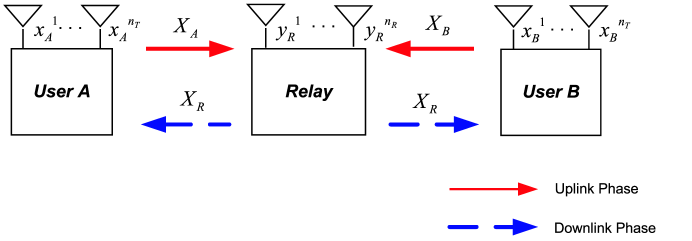
Figure 1: Configuration of a MIMO TWRC.

A MIMO TWRC, in which user $A$ and user $B$ exchange information via a relay, is illustrated in Fig. 1. Each user is equipped with $n_{T}$ antennas and the relay has $n_{R}$ antennas. All the channels in the system are assumed to be flat-fading within the bandwidth of interest. The channel from user $A$ $($or $B)$ to the relay is denoted by an $n_{R}$-by-$n_{T}$ matrix $\mathbf{H}_{A,R}$ $\left(\text{or }\mathbf{H}_{B,R}\right)$. The channel from the relay to user $A$ $($or $B)$ is denoted by an $n_{T}$-by-$n_{R}$ matrix $\mathbf{H}_{R,A}$ $\left(\text{or }\mathbf{H}_{R,B}\right)$.

The users and the relay operate in half-duplex mode. There is no direct link between the two users. The transmission protocol employs two consecutive equal-duration time-slots for each round of information exchange between the users via the relay. Each time-slot consists of $n$ channel users. In the first time-slot (uplink phase), the two users transmit to the relay simultaneously and the relay remains silent. In the second time-slot (downlink phase), the relay broadcasts to the two silent users. We assume that the channel coefficients remain the same for each round of information exchange. We also assume that the channel matrices are globally known by both users, as well as by the relay.

In this paper, we will only consider the situation of $n_{T}$ $\geq$ $n_{R}$. This configuration applies to practical scenarios such as a wireless sensor network where the physical sizes of the intermediate sensor nodes are smaller than those of the terminal nodes.

II-B Uplink Phase

The discrete channel of the uplink phase can be written as

$$Y_{R}\left[l\right]=\mathbf{H}_{A,R}X_{A}\left[l\right]+\mathbf{H}_{B,R}X_{B}\left[l\right]+Z_{R}\left[l\right],\text{ }l=1,\cdots,n,$$ (1)

where $X_{m}\left[l\right]$ is an $n_{T}$-by-1 column vector with the $i$th entry $x_{m,i}\left[l\right],i=1,\cdots,n_{T}$, being the coded signal transmitted from antenna $i$ of user $m$, $m\in\left\{A,B\right\}$, at time instant $l$; $Y_{R}\left[l\right]$ is an $n_{R}$-by-1 column vector with the $j$th entry $y_{R,j}\left[l\right],j=1,\cdots,n_{R}$, being the signal received from antenna $j$ of the relay; $Z_{R}\left[l\right]$ is an $n_{R}$-by-1 additive white Gaussian noise (AWGN) vector at the relay with the $j$th entry $z_{R,j}\left[l\right]\sim\mathcal{N}\left(0,\sigma_{R}^{2}\right),$ $j=1,\cdots,n_{R}$, where $\sigma_{R}^{2}$ is the noise variance. For notational simplicity, the time index $l$ may be omitted in situations without causing ambiguity.

The channel input covariances of the two users are denoted by $\mathbf{Q}_{m}=\mathcal{E}\left(X_{m}X_{m}^{T}\right),m\in\left\{A,B\right\}$, where $\mathcal{E}\left(\cdot\right)$ stands for the expectation operation. The power constraint of the uplink phase is given by

$$\text{Tr}\left\{\mathbf{Q}_{A}+\mathbf{Q}_{B}\right\}\leq P_{T}$$ (2)

where $P_{T}$ is the total transmission power of the two users. The average per-user SNR of the uplink phase is defined as

$$SNR\triangleq\frac{P_{T}}{2\sigma_{R}^{2}}.$$ (3)

II-C Relay’s Operation

Upon receiving $\mathbf{Y}_{R}=\left[Y_{R}\left[1\right],\cdots,Y_{R}\left[n\right]\right]$, the relay generates a signal matrix $\mathbf{X}_{R}=\left[X_{R}\left[1\right],\cdots,X_{R}\left[n\right]\right]$. Here, $X_{R}\left[l\right]$ is an $n_{R}$-by-$1$ real vector with the $j$th entry $x_{R,j}\left[l\right]$, $j=1,\cdots,n_{R}$, being the signal transmitted from the $j$th antenna of the relay, at time instant $l$, in the downlink phase. In general, the relationship between $\mathbf{X}_{R}$ and $\mathbf{Y}_{R}$ can be written as

$$\mathbf{X}_{R}=f_{R}\left(\mathbf{Y}_{R}\right)$$ (4)

where $f_{R}\left(\cdot\right)$ denotes the relay’s functionality. The relay’s power constraint is given by

$$\text{Tr}\left\{\mathbf{Q}_{R}\right\}\leq P_{R}$$ (5)

where $\mathbf{Q}_{R}=\mathcal{E}\left(X_{R}X_{R}^{T}\right)\$denotes the channel input covariance matrix of the relay in the downlink phase.

Remark 1

In this paper, the power constraints under consideration are given by $\left(\ref{Eq_PowerConstraint}\right)$ and $\left(\ref{Eq_RelayPowerConstraint}\right)$. The generalization to the case with a global sum-power constraint can be readily done by trading off the portion of power allocated to the users and that to the relay.

II-D Downlink Phase

During the downlink phase, the signal $\mathbf{X}_{R}=\left[X_{R}\left[1\right],\cdots,X_{R}\left[n\right]\right]$ serves as the channel input and is broadcast to users $A$ and $B$. The signals received by user $m$, $m\in\left\{A,B\right\},$ are given by

$$Y_{m}\left[l\right]=\mathbf{H}_{R,m}X_{R}\left[l\right]+Z_{m}\left[l\right],l=1,\cdots,n,$$ (6)

where $Z_{m}\left[l\right]$ is an $n_{T}$-by-1 AWGN vector with the $i$th entry $z_{m,i}\left[l\right]\sim\mathcal{N}\left(0,\sigma_{m}^{2}\right)$, $i=1,\cdots,n_{T}$, where $\sigma_{m}^{2}$ is the noise variance at user $m$. Upon receiving $\mathbf{Y}_{A}=\left[Y_{A}\left[1\right],\cdots,Y_{A}\left[n\right]\right]$, user $A$ decodes user $B$’s message with the help of the perfect knowledge of $\mathbf{X}_{A}=\left[X_{A}\left[1\right],\cdots,X_{A}\left[n\right]\right]$. Meanwhile, similar operations are performed by user $B$. This finishes one round of information exchange.

For notational simplicity, we assume $\sigma_{R}^{2}=\sigma_{A}^{2}=\sigma_{B}^{2}=1$ in this paper. Then, the average per-user SNR is $SNR=P_{T}/2$ and the SNR of the relay is $SNR_{R}=$ $P_{R}$. The extension of our results to the case of unequal noise power is straightforward.

III Capacity Upper Bound and Existing Schemes for a MIMO TWRC

III-A Definitions

The achievable rate-pair and rate-region of a MIMO TWRC are defined as follows:

Definition 1

A rate-pair $\left(R_{A}\text{, }R_{B}\right)$ is said to be achievable if there exists a set of $2^{nR_{A}}$ codewords for user $A$, a set of $2^{nR_{B}}$ codewords for user $B$ and a relay functionality $\mathbf{X}_{R}=f_{R}\left(\mathbf{Y}_{R}\right),$ satisfying power constraints (2) and (5), such that the decoding error probabilities approach zero at both user nodes of the TWRC, as $n\rightarrow\infty$.

Remark 2

The rate of each user is defined as the amount of transmitted bits in each transmission round, normalized by the duration of one phase (consisting of $n$ channel uses).

Definition 2

The achievable rate-region $\mathcal{R}$ is defined as the convex closure of all achievable rate-pairs.

III-B Capacity Upper Bound of a MIMO TWRC

We now derive a new capacity upper bound (UB) for a MIMO TWRC. We present the result in the following lemma, which is an extension of the cut-set bound for a SISO TWRC [2].

Lemma 1

For given input covariance matrices $\mathbf{Q}_{A},$ $\mathbf{Q}_{B}$ and $\mathbf{Q}_{R}$, the achievable rate-pair of a MIMO TWRC is upper bounded by

$$R_{A}\leq R_{A}^{UB}=\frac{1}{2}\min\left[\log\det\left(\mathbf{I}+\mathbf{H}_{A,R}\mathbf{Q}_{A}\mathbf{H}_{A,R}^{T}\right)\text{, }\log\det\left(\mathbf{I}+\mathbf{H}_{R,B}\mathbf{Q}_{R}\mathbf{H}_{R,B}^{T}\right)\right]$$ (7a)

$$R_{B}\leq R_{B}^{UB}=\frac{1}{2}\min\left[\log\det\left(\mathbf{I}+\mathbf{H}_{B,R}\mathbf{Q}_{B}\mathbf{H}_{B,R}^{T}\right)\text{, }\log\det\left(\mathbf{I}+\mathbf{H}_{R,A}\mathbf{Q}_{R}\mathbf{H}_{R,A}^{T}\right)\right].$$ (7b)

Proof:

From the cut-set bound, the achievable rate-pair of a TWRC is upper-bounded by [2]

$$R_{A}\leq R_{A}^{UB}=\min\left\{I(X_{A};Y_{R}|X_{B}),I(X_{R};Y_{B})\right\},$$ (8a)

$$R_{B}\leq R_{B}^{UB}=\min\left\{I(X_{B};Y_{R}|X_{A}),I(X_{R};Y_{A})\right\}.$$ (8b)

Applying the capacity formula of a real-valued MIMO channel [12] for given input covariances $\mathbf{Q}_{A},$ $\mathbf{Q}_{B}$ and $\mathbf{Q}_{R}$, we obtain (7).    

With the result in Lemma 1, the capacity UB of a MIMO TWRC can be determined by optimizing the covariance matrices $\mathbf{Q}_{A},$ $\mathbf{Q}_{B}$ and $\mathbf{Q}_{R}$. This capacity UB provides an upper limit on the data rate that any MIMO two-way relay scheme can achieve.

III-C Analog Network Coding for a MIMO TWRC

Much progress has been made in developing communication strategies to approach the capacity of a MIMO TWRC. Among those, an AF-based scheme, namely analog network coding (ANC) [4]-[6], has attracted a great deal of attention. In ANC, the relay broadcasts an amplified version of its received signal to the two users. The maximum achievable rate of ANC in MIMO TWRC remains unsolved and a sub-optimal solution is reported in [6]. In this paper, we will consider the upper bound of the achievable rate of ANC, derived in [33], as a benchmark for comparison purpose.

The ANC scheme has two disadvantages. First, it suffers from noise amplification, since the noise received by the relay is not suppressed before the signal is forwarded to the users. Second, it suffers from unnecessary power consumption at the relay, since the AF relay forwards a linear, rather than an algebraic, superposition of the signals from the two users [1].

III-D DF with Network Coding for a MIMO TWRC

A DF-based scheme has also been studied for a MIMO TWRC [7], [17]. In the DF-based scheme, the relay completely decodes both users’ messages. The decoded messages of two users are re-encoded with a network code [1], [9], and a channel code. The resultant coded signal is broadcast to the two users in the downlink phase. We refer to this scheme as DF with network coding (DF-NC).

The achievable rate of the DF-NC scheme is briefly discussed as follows. The uplink phase of DF-NC can be viewed as a MIMO multiple-access channel whose exact achievable rate-region is still an open problem, although its upper and lower bounds are studied in [20]. We will use the upper bound in [20] for comparison purpose. The downlink rate-region of the DF-NC scheme can be obtained by extending the result in [2] to a MIMO scenario. The overall achievable rate-region of the DF-NC scheme is the intersection of the uplink and downlink rate-regions determined above.

The DF-NC scheme suffers from a severe multiplexing loss [3], [7], as complete decoding at the relay is demanding and unnecessary. As a result, the achievable rate of the DF-NC scheme may far below the capacity of a MIMO TWRC, especially in the high SNR region [7].

IV Eigen-Direction Alignment Based Physical-Layer Network Coding

In this section, we propose a new strategy for MIMO TWRCs. The proposed strategy consists of two key components: eigen-direction alignment (EDA) precoding and physical-layer network coding (PNC). In particular, the proposed EDA precoding algorithm efficiently aligns the eigen-directions of two users. Then, we carry out multi-stream PNC over the aligned eigen-modes established by the EDA precoding.

To illustrate the proposed EDA precoding algorithm, we first describe a straightforward (naive) method to perform the eigen-direction alignment.

IV-A A Naive Eigen-Direction Alignment Approach

Denote by $\mathbf{F}_{A}$ and $\mathbf{F}_{B}$ the linear precoding matrices of user $A$ and user $B$, respectively. The users’ transmitted signals can be written as

$$X_{m}\left[l\right]=\mathbf{F}_{m}C_{m}\left[l\right],m\in\left\{A,B\right\},l=1,\cdots,n,$$ (9)

where $C_{m}\left[l\right]=\left[c_{m,1}\left[l\right],\cdots,c_{m,n_{R}}\left[l\right]\right]^{T}$, $\mathcal{E}\left(C_{m}C_{m}^{T}\right)=\mathbf{I}$, is a length-$n_{R}$ column vector whose entries denote the independently coded signals. As a straightforward approach, the precoder performs channel inverse, i.e., $\mathbf{F}_{m}$ is given by

$$\mathbf{F}_{m}=\mathbf{H}_{m,R}^{T}\left(\mathbf{H}_{m,R}\mathbf{H}_{m,R}^{T}\right)^{-1}\mathbf{\Psi}_{m},m\in\left\{A,B\right\},$$ (10)

where $\mathbf{H}_{m,R}^{T}\left(\mathbf{H}_{m,R}\mathbf{H}_{m,R}^{T}\right)^{-1}$ is the Moore-Penrose pseudo-inverse of $\mathbf{H}_{m,R}$ (for $n_{T}\geq n_{R}$) and $\mathbf{\Psi}_{m}$ is an $n_{R}\times n_{R}$ diagonal matrix which allocates power among the $n_{R}$ eigen-modes for user $m$. With (10), the signal received by the relay in (1) can be written as

$$Y_{R}\left[l\right] =\mathbf{H}_{A,R}\mathbf{F}_{A}C_{A}\left[l\right]+\mathbf{H}_{B,R}\mathbf{F}_{B}C_{B}\left[l\right]+Z_{R}\left[l\right]$$ (11a)

$$=\mathbf{\Psi}_{A}C_{A}\left[l\right]+\mathbf{\Psi}_{B}C_{B}\left[l\right]+Z_{R}\left[l\right].$$ (11b)

Eq. (11b) represents $n_{R}$ parallel sub-channels, as both $\mathbf{\Psi}_{A}$ and $\mathbf{\Psi}_{B}$ are diagonal matrices. The above approach is referred to as a naive EDA precoding. Unfortunately, it is well-known that the channel inverse in precoding suffers from a significant power loss when the channel matrix is ill-conditioned [12]. Thus, this approach may not be an efficient method to align the eigen-directions.

IV-B Proposed Eigen-Direction Alignment Precoding

Now, we propose our new EDA precoding algorithm which can effectively avoid the power loss suffered by the naive EDA precoder. Consider an invertible linear transformation of the relay’s received signal as

$$\widetilde{Y}_{R}\left[l\right] = \mathbf{K}^{-1}Y_{R}\left[l\right]$$

$$= \mathbf{K}^{-1}\mathbf{H}_{A,R}X_{A}\left[l\right]+\mathbf{K}^{-1}\mathbf{H}_{B,R}X_{B}\left[l\right]+\mathbf{K}^{-1}Z_{R}\left[l\right],\text{ }l=1,\cdots,n,$$

where $\mathbf{K}$ is an $n_{R}$-by-$n_{R}$ invertible square matrix referred to as the rotation matrix. The equivalent channel matrices are now given by

$$\widetilde{\mathbf{H}}_{m,R}=\mathbf{K}^{-1}\mathbf{H}_{m,R},m\in\left\{A,B\right\}.$$ (13)

Applying the aforementioned naive EDA precoding over the equivalent channel in (13), we obtain the proposed new EDA precoding matrix as

$$\mathbf{F}_{m} = \widetilde{\mathbf{H}}_{m,R}^{T}\left(\widetilde{\mathbf{H}}_{m,R}\widetilde{\mathbf{H}}_{m,R}^{T}\right)^{-1}\mathbf{\Psi}_{m}$$ (14)

$$= \mathbf{H}_{m,R}^{T}\left(\mathbf{H}_{m,R}\mathbf{H}_{m,R}^{T}\right)^{-1}\mathbf{K\Psi}_{m},m\in\left\{A,B\right\}.$$

The signal received by the relay in (1) can then be written as

$$Y_{R}\left[l\right]=\mathbf{H}_{A,R}\mathbf{F}_{A}C_{A}\left[l\right]+\mathbf{H}_{B,R}\mathbf{F}_{B}C_{B}\left[l\right]+Z_{R}\left[l\right]=\mathbf{K}\left(\mathbf{\Psi}_{A}C_{A}\left[l\right]+\mathbf{\Psi}_{B}C_{B}\left[l\right]\right)+Z_{R}\left[l\right]$$ (15)

where $l=1,\cdots,n$. At the relay, after the linear transformation (IV-B), we obtain

$$\widetilde{Y}_{R}\left[l\right]=\mathbf{\Psi}_{A}C_{A}\left[l\right]+\mathbf{\Psi}_{B}C_{B}\left[l\right]+\widetilde{Z}_{R}\left[l\right]$$ (16)

where $\widetilde{Z}_{R}\left[l\right]=\mathbf{K}^{-1}Z_{R}\left[l\right]$ is the equivalent noise vector. From (16), it is clear that $n_{R}$ aligned eigen-modes are established. Note that we can always scale the entries of $\widetilde{Y}_{R}$ such that the equivalent noises of all eigen-modes have unit power. Thus, without loss of generality, we confine the rotation matrix $\mathbf{K}$ that the diagonal elements of $\mathbf{K}^{-1}\left(\mathbf{K}^{-1}\right)^{T}$ are 1, i.e.,

$$\left[\mathbf{K}^{-1}\left(\mathbf{K}^{-1}\right)^{T}\right]_{\text{diag}}=\mathbf{I}\text{.}$$ (17)

This is to ensure that the entries in the effective noise vector $\widetilde{Z}_{R}\left[l\right]$ have unit power.

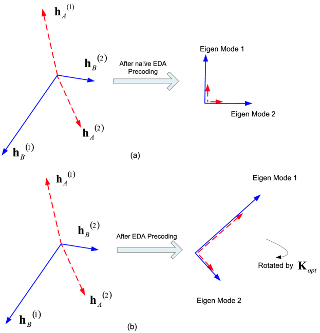
Figure 2: Geometrical illustration of (a) Naive EDA precoding and (b) EDA precoding (with $\mathbf{KK}^{T}=\mathbf{I}$), for a two dimension case. Here, $\mathbf{H}_{m,R}=[\mathbf{h}_{m}^{\left(1\right)},\mathbf{h}_{m}^{\left(2\right)}],m\in\left\{A,B\right\}$. The dashed arrow and solid arrow denote users $A$ and $B$, respectively. For $A$, since the correlation of its channel vectors is large, a significant power loss is suffered in the naive EDA precoding. The proposed EDA precoding can effectively avoid this loss by introducing a rotation.

The proposed EDA precoding scheme reduces to the naive EDA scheme by letting $\mathbf{K}$ $=\mathbf{I}$. By varying the rotation matrix $\mathbf{K}$, we can actually align the eigen-modes of the two users into any $n_{R}$ pre-determined directions in the $n_{R}$-dimension vector space, as illustrated in Fig. 2. An immediate question is how to determined the optimal rotation matrix $\mathbf{K}$. We will retain the answer to this problem till the next section.

IV-C The Overall Proposed EDA-PNC Scheme

We now describe a multi-stream PNC scheme. In the uplink phase, the proposed EDA precoding (14) is employed to establish $n_{R}$ aligned parallel sub-channels. The two users perform single-stream PNC for each aligned sub-channel, and there are $n_{R}$ independent PNC streams in total. Similarly to the case of SISO PNC [2], the relay recovers the $n_{R}$ bin-indices (as defined in [2]) instead of completely decoding both users’ individual messages. In the downlink phase, the aggregation of the $n_{R}$ bin-indices is re-encoded and broadcast to the two users. Finally, each user recovers the other user’s message with the help of the perfect knowledge of its own message.

V Achievable Rates of the Proposed EDA-PNC Scheme for MIMO TWRCs

V-A Achievable Rate-Pair

We now present a theorem on the achievable rate-pair of the proposed EDA-PNC scheme. Define $x^{+}\triangleq\max\left(x,0\right).$

Theorem 1

For given $\mathbf{K}$, $\mathbf{\Psi}_{A}$, $\mathbf{\Psi}_{B}$ and $\mathbf{Q}_{R}$, an achievable rate-pair of the proposed EDA-PNC scheme is given by

$$R_{A} \leq\min\left\{R_{A,UL}^{EDA},R_{A,DL}^{EDA}\right\}$$ (18a)

$$R_{B} \leq\min\left\{R_{B,UL}^{EDA},R_{B,DL}^{EDA}\right\}$$ (18b)

where

$$R_{A,UL}^{EDA} =\frac{1}{2}\mathop{\displaystyle\sum}\limits_{i=1}^{n_{R}}\left[\log\left(\frac{\Psi_{A}\left(i,i\right)^{2}}{\Psi_{A}\left(i,i\right)^{2}+\Psi_{B}\left(i,i\right)^{2}}+\Psi_{A}\left(i,i\right)^{2}\right)\right]^{+},$$ (19a)

$$R_{B,UL}^{EDA} =\frac{1}{2}\mathop{\displaystyle\sum}\limits_{i=1}^{n_{R}}\left[\log\left(\frac{\Psi_{B}\left(i,i\right)^{2}}{\Psi_{A}\left(i,i\right)^{2}+\Psi_{B}\left(i,i\right)^{2}}+\Psi_{B}\left(i,i\right)^{2}\right)\right]^{+},$$ (19b)

$$R_{A,DL}^{EDA} =\frac{1}{2}\log\det\left(\mathbf{I}+\mathbf{H}_{R,B}\mathbf{Q}_{R}\mathbf{H}_{R,B}^{T}\right),$$ (19c)

$$R_{B,DL}^{EDA} =\frac{1}{2}\log\det\left(\mathbf{I}+\mathbf{H}_{R,A}\mathbf{Q}_{R}\mathbf{H}_{R,A}^{T}\right).$$ (19d)

The proof of Theorem 1 is given in Appendix II. The main idea of the proof is to utilize the results on nested lattice codes in [2].

V-B An Asymptotic Result on the Achievable Rate-Pair

We next derive an asymptotic result which is based on the following observation.

Fact 1

Assume that the entries of the channel matrix $\mathbf{H}_{m,R}$ are i.i.d. with zero mean and unit variance. Then,

$$\frac{1}{n_{T}}\mathbf{H}_{m,R}\mathbf{H}_{m,R}^{T}\overset{\text{P}}{\rightarrow}\mathbf{I}\text{, as }n_{T}\rightarrow\mathbf{\infty,}$$ (20)

where “$\overset{\text{P}}{\rightarrow}$” represents convergence in probability.

The above result is straightforward by invoking the weak law of large numbers.

Theorem 2

Assume that the channel coefficients in $\mathbf{H}_{A,R}$ and $\mathbf{H}_{B,R}$ are i.i.d. withe zero mean and unit variance. As $n_{T}$ tends to infinity (while $n_{R}$ remains finite), the proposed EDA-PNC scheme asymptotically achieves the capacity of a MIMO TWRC in probability. $\square$

The proof of Theorem 2 is given in Appendix III. Theorem 2 states that the proposed EDA-PNC scheme achieves the capacity upper bound of a MIMO TWRC with probability 1 as $n_{T}\rightarrow\mathbf{\infty}$. This asymptotic result will be verified by the numerical results presented later.

V-C Determining the Achievable Rate-Region

Here, we consider the achievable rate-region of the proposed EDA-PNC scheme, based on the results of Theorem 1. Define the following rate-regions

$$\mathcal{R}_{UL}^{EDA} \triangleq \left\{\left(R_{A},R_{B}\right):R_{A}\leq R_{A,UL}^{EDA},R_{B}\leq R_{B,UL}^{EDA}\right\},$$ (21a)

$$\mathcal{R}_{DL}^{EDA} \triangleq \left\{\left(R_{A},R_{B}\right):R_{A}\leq R_{A,DL}^{EDA},R_{B}\leq R_{B,DL}^{EDA}\right\}.$$ (21b)

The above two rate-regions will be respectively determined in the following.

V-C1 Uplink Rate-Region

The boundary of the uplink rate-region $\mathcal{R}_{UL}^{EDA}$ can be determined by solving the following weighted sum-rate (WSR) problem

$$\max_{\mathbf{K,\Psi}_{A},\text{ }\mathbf{\Psi}_{B}}\left\{\alpha R_{A,UL}^{EDA}+\left(1-\alpha\right)R_{B,UL}^{EDA}\right\}$$ (22a)

subject to

$$\text{Tr}\left(\left(\mathbf{H}_{A,R}\mathbf{H}_{A,R}^{T}\right)^{-1}\mathbf{K\Psi}_{A}^{2}\mathbf{K}^{T}+\left(\mathbf{H}_{B,R}\mathbf{H}_{B,R}^{T}\right)^{-1}\mathbf{K\Psi}_{B}^{2}\mathbf{K}^{T}\right)\leq P_{T}.$$ (22b)

and (17), for $0\leq\alpha\leq 1$. Note that the power constraint in (22b) is obtained by substituting (14) and $\mathbf{Q}_{m}=\mathbf{F}_{m}\mathbf{F}_{m}^{T}$, $m\in\left\{A,B\right\}$, into (2).

The problem in (22) is non-convex and hence is difficult to solve. For a small $n_{R}$, e.g., $n_{R}=2$, the optimal parameters $\left(\mathbf{K,\Psi}_{A},\mathbf{\Psi}_{B}\right)$ can be found by an exhaustive search. Unfortunately, this method quickly becomes prohibitively complex as $n_{R}$ increases. We will provide approximate solutions to this problem in Section VI.

V-C2 Downlink Rate-Region

The boundary of the downlink rate-region $\mathcal{R}_{DL}^{EDA}$ can be determined by solving

$$\max_{\mathbf{Q}_{R}:\text{ Tr}\left(\mathbf{Q}_{R}\right)\leq P_{R}}\left\{\alpha R_{A,DL}^{EDA}+\left(1-\alpha\right)R_{B,DL}^{EDA}\right\}$$ (23)

for $0\leq\alpha\leq 1$. Note that $\log\det\left(\cdot\right)\$is concave and thus the objective function in (23) is concave in $\mathbf{Q}_{R}$. In addition, Tr$\left(\mathbf{Q}_{R}\right)\leq P_{R}$ is a linear constraint. Therefore, (23) can be solved using convex optimization.

V-C3 Overall Rate-Region

The overall achievable rate-region of the proposed EDA-PNC scheme is the intersection of $\mathcal{R}_{UL}^{EDA}$ and $\mathcal{R}_{DL}^{EDA}$.

The major difficulty in determining the above achievable rate-region of the proposed EDA-PNC scheme is to solve the WSR problem in (22). In the next section, we will provide two suboptimal solutions to this problem.

VI Approximate Solutions to the Optimal EDA Precoder

VI-A Approximate Solution I

To simplify the problem in (22), we introduce two extra constraints on the proposed EDA precoder: 1) The rotation matrix $\mathbf{K}$ is unitary, i.e.,

$$\mathbf{KK}^{T}=\mathbf{I},$$ (24)

and 2) The power matrices satisfy

$$\mathbf{\Psi}_{A}=\mathbf{\Sigma},\text{ }\mathbf{\Psi}_{B}=\gamma\mathbf{\Sigma},$$ (25)

where $\gamma$ is a positive scalar and $\mathbf{\Sigma}$ is a diagonal matrix with non-negative diagonal elements. Although these extra constraints may lead to a certain performance loss, a close-form solution then exists, which yields crucial insights into the design of the EDA precoder. Later, we will consider the relaxation of these two constraints to obtain a better approximate solution.

VI-A1 Optimal Unitary Rotation Matrix $\mathbf{K}$ (for $\mathbf{\Psi}_{B}=\gamma\mathbf{\Psi}_{A}$)

Now we derive the most power-efficient unitary rotation matrix $\mathbf{K}$ for given $\mathbf{\Psi}_{A}=\mathbf{\Sigma}$ and $\mathbf{\Psi}_{B}=\gamma\mathbf{\Sigma}$. The problem is formulated as

$$\mathbf{K}_{opt}^{(\mathbf{\Sigma},\gamma)}=\arg\min_{\mathbf{K:}\text{ }\mathbf{KK}^{T}=\mathbf{I}}\text{Tr}\left(\mathbf{F}_{A}\mathbf{F}_{A}^{H}+\mathbf{F}_{B}\mathbf{F}_{B}^{H}\right)$$ (26)

Let the singular value decomposition (SVD) of the channel matrix $\mathbf{H}_{m,R}$ be

$$\mathbf{H}_{m,R}=\mathbf{U}_{m}\mathbf{\Sigma}_{m}\mathbf{V}_{m}^{T},\text{ }m\in\left\{A,B\right\},$$ (27)

where $\mathbf{U}_{m}$ and $\mathbf{V}_{m}^{T}$ are unitary matrices and $\mathbf{\Sigma}_{m}$ is an $n_{R}$-by-$n_{T}$ diagonal matrix with positive diagonal elements. Denote by $\mathbf{\Sigma}_{m}^{-1}$ the pseudo-inverse of $\mathbf{\Sigma}_{m}$, i.e.,

$$\mathbf{\Sigma}_{m}^{-1}=\left[\begin{array}[]{c}\mathbf{\Upsilon}_{m}^{-1}\\ \mathbf{0}_{(n_{T}-n_{R})\times n_{R}}\end{array}\right]$$

where $\mathbf{\Upsilon}_{m}$ is an $n_{R}$-by-$n_{R}$ matrix formed by the first $n_{R}$ columns of $\mathbf{\Sigma}_{m}$ and $\mathbf{0}_{(n_{T}-n_{R})\times n_{R}}$ denotes an $(n_{T}-n_{R})$-by-$n_{R}$ matrix with all-zero entries. For notational simplicity, we denote $\left(\mathbf{\Sigma}_{m}\mathbf{\Sigma}_{m}^{T}\right)^{-1}$ by $\mathbf{\Sigma}_{m}^{-2}$. Then, using (14) and (27), the problem (26) becomes

$$\mathbf{K}_{opt}^{(\mathbf{\Sigma},\gamma)}=\arg\min_{\mathbf{K:}\text{ }\mathbf{KK}^{T}=\mathbf{I}}\text{Tr}\left(\left(\mathbf{U}_{A}\mathbf{\Sigma}_{A}^{-2}\mathbf{U}_{A}^{T}+\gamma^{2}\mathbf{U}_{B}\mathbf{\Sigma}_{B}^{-2}\mathbf{U}_{B}^{T}\right)\mathbf{K\Sigma K}^{T}\right).$$ (28)

Define

$$\mathbf{G}\left(\gamma\right)\triangleq\mathbf{U}_{A}\mathbf{\Sigma}_{A}^{-2}\mathbf{U}_{A}^{T}+\gamma^{2}\mathbf{U}_{B}\mathbf{\Sigma}_{B}^{-2}\mathbf{U}_{B}^{T}.$$ (29)

The eigen-decomposition of $\mathbf{G}\left(\gamma\right)$ yields $\mathbf{G}\left(\gamma\right)=\mathbf{U}_{G\left(\gamma\right)}\mathbf{\Lambda}_{G\left(\gamma\right)}\mathbf{U}_{G\left(\gamma\right)}^{T}$ where $\mathbf{\Lambda}_{G\left(\gamma\right)}$ is a diagonal matrix with the diagonal entries arranged in the ascending order, and $\mathbf{U}_{G\left(\gamma\right)}$ is a unitary matrix. Without loss of generality, we always assume that the diagonal entries of $\mathbf{\Sigma}$ are arranged in the descending order. Now, we present the optimal unitary rotation matrix $\mathbf{K}$ in the following theorem.

Theorem 3

For any given $\mathbf{\Psi}_{A}=\mathbf{\Sigma}$ and $\mathbf{\Psi}_{B}=\gamma\mathbf{\Sigma}$, the solution to the problem in (28) is

$$\mathbf{K}_{opt}^{(\gamma)}=\mathbf{U}_{G\left(\gamma\right)}.$$ (30)

Proof:

With (29), the objective function in (28) is written as

$$\text{Tr}\left(\mathbf{G}\left(\gamma\right)\mathbf{K\Sigma}^{2}\mathbf{K}^{T}\right)=\text{Tr}\left(\mathbf{U}_{G\left(\gamma\right)}\mathbf{\Lambda}_{G\left(\gamma\right)}\mathbf{U}_{G\left(\gamma\right)}^{T}\mathbf{K\Sigma}^{2}\mathbf{K}^{T}\right)\leq\text{Tr}\left(\mathbf{\Lambda}_{G\left(\gamma\right)}\mathbf{\Sigma}^{2}\right).$$ (31)

where the equality in the last step holds when $\mathbf{K=U}_{G\left(\gamma\right)}$. The inequality in (31) follows the fact [21], [32]: for any two hermitian matrix $\mathbf{M}$ and $\mathbf{N}$ with eigen decomposition $\mathbf{M}=\mathbf{U}_{M}\mathbf{\Lambda}_{M}\mathbf{U}_{M}^{T}$ and $\mathbf{N}=\mathbf{U}_{N}\mathbf{\Lambda}_{N}\mathbf{U}_{N}^{T}$,

$$\text{Tr}\left(\mathbf{MN}\right)\leq\text{Tr}\left(\mathbf{\Lambda}_{M}\mathbf{\Lambda}_{N}\right)$$ (32)

where the diagonal elements of $\mathbf{\Lambda}_{M}$ and those $\mathbf{\Lambda}_{N}$ are reversely ordered. This finishes the proof.    

We have the following comments on Theorem 3.

Remark 3

The optimal unitary rotation matrix $\mathbf{K}_{opt}^{(\gamma)}$ is dependent of $\gamma$, but not of $\mathbf{\Sigma}$. Thus, we write $\mathbf{K}_{opt}^{(\gamma)}$ instead of $\mathbf{K}_{opt}^{(\mathbf{\Sigma},\gamma)}$.

Remark 4

With $\mathbf{K}_{opt}^{(\gamma)}=\mathbf{U}_{G\left(\gamma\right)}$, the power constraint in (2) can be expressed as

$$\text{Tr}\left[\mathbf{G}\left(\gamma\right)\mathbf{K}_{opt}^{(\gamma)}\mathbf{\Sigma}^{2}\left(\mathbf{K}_{opt}^{(\gamma)}\right)^{T}\right]=\text{Tr}\left(\mathbf{\Lambda}_{G\left(\gamma\right)}\mathbf{\Sigma}^{2}\right)\leq P_{T}\text{.}$$ (33)

VI-A2 Uplink Rate-Region Revisited

Here, we present an approximate solution to the the uplink achievable rate-region $\mathcal{R}_{UL}^{EDA}$ of the proposed EDA-PNC scheme. With $\mathbf{\Psi}_{A}=\mathbf{\Sigma}$ and $\mathbf{\Psi}_{B}=\gamma\mathbf{\Sigma}$, (19a) and (19b) become

$$\widetilde{R}_{A,UL}^{EDA} =\frac{1}{2}\mathop{\displaystyle\sum}\limits_{i=1}^{n_{R}}\left[\log\left(\frac{1}{1+\gamma^{2}}+\Sigma\left(i,i\right)^{2}\right)\right]^{+},$$ (34a)

$$\widetilde{R}_{B,UL}^{EDA} =\frac{1}{2}\mathop{\displaystyle\sum}\limits_{i=1}^{n_{R}}\left[\log\left(\frac{\gamma^{2}}{1+\gamma^{2}}+\gamma^{2}\Sigma\left(i,i\right)^{2}\right)\right]^{+}$$ (34b)

where $\Sigma\left(i,i\right)$ denotes the $i$th diagonal entry of $\mathbf{\Sigma}$.

Correspondingly, the WSR problem in (22) becomes

$$\max_{\mathbf{\Sigma},\text{ }\gamma,\mathbf{K}}\left\{\alpha\widetilde{R}_{A,UL}^{EDA}+\left(1-\alpha\right)\widetilde{R}_{B,UL}^{EDA}\right\}$$ (35a)

subject to

$$\text{Tr}(\mathbf{G}\left(\gamma\right)\mathbf{K\Sigma}^{2}\mathbf{K}^{T})\leq P_{T}\text{ and }\mathbf{KK}^{T}=\mathbf{I.}$$ (35b)

For the above problem, if the optimal $\left(\mathbf{K},\mathbf{\Sigma}\right)$ couple for any given $\gamma$ can be found, the optimal solution to (35) can be easily determined by a one-dimension full search over $\gamma$.

We next determine the optimal $\left(\mathbf{K},\mathbf{\Sigma}\right)$ couple for an arbitrarily given $\gamma$. The optimal unitary rotation matrix $\mathbf{K}$ to the problem in (35), for a given $\gamma$, is presented in the following lemma (which is a direct result of Theorem 3).

Lemma 2

Given $\gamma$, the optimal $\mathbf{K}$ to the maximum WSR problem in (35) is $\mathbf{K}_{opt}^{(\gamma)}=\mathbf{U}_{G\left(\gamma\right)}$ given in (30).

The remaining task is to find the optimal diagonal matrix $\mathbf{\Sigma}$. The optimization problem in (35a) can be equivalently written as

$$\max_{\mathbf{\Sigma}}\left\{\frac{\alpha}{2}\mathop{\displaystyle\sum}\limits_{i=1}^{n_{R}}\left[\log\left(\frac{1}{1+\gamma^{2}}+\Sigma\left(i,i\right)^{2}\right)\right]^{+}+\frac{1-\alpha}{2}\mathop{\displaystyle\sum}\limits_{i=1}^{n_{R}}\left[\log\left(\frac{\gamma^{2}}{1+\gamma^{2}}+\gamma^{2}\Sigma\left(i,i\right)^{2}\right)\right]^{+}\right\}$$ (36)

subject to Tr$\left(\mathbf{\Lambda}_{G\left(\gamma\right)}\mathbf{\Sigma}^{2}\right)\leq P_{T}$ (cf., (33)).

The objective function (36) involves $[\cdot]^{+}$ operations, and thus is not concave. However, if we know in advance which $[\cdot]^{+}$ operations should be activated, (36) can be converted into a convex optimization problem. Consider any two index subsets $S_{m}\subseteq$ $\{1,\ldots,n_{R}\}$, $m\in\left\{A,B\right\}$. We formulate the following problem

$$\max_{\mathbf{\Sigma}}\left\{\frac{\alpha}{2}\mathop{\displaystyle\sum}\limits_{i\in S_{A}}\left[\log\left(\frac{1}{1+\gamma^{2}}+\Sigma\left(i,i\right)^{2}\right)\right]+\frac{1-\alpha}{2}\mathop{\displaystyle\sum}\limits_{i\in S_{B}}\left[\log\left(\frac{\gamma^{2}}{1+\gamma^{2}}+\gamma^{2}\Sigma\left(i,i\right)^{2}\right)\right]\right\}$$ (37)

subject to Tr$\left(\mathbf{\Lambda}_{G\left(\gamma\right)}\mathbf{\Sigma}^{2}\right)\leq P_{T}$. The solution to the above problem is given in the following lemma, with the proof given in Appendix IV.

Lemma 3

For given $S_{A}$, $S_{B}$ and $\gamma$, the solution to the problem in (37) is given by

$$\Sigma_{opt}^{\left(S_{A},S_{B},\gamma\right)}(i,i)=\left\{\begin{array}[]{cc}\sqrt{\left(\frac{1}{2\lambda\Lambda_{G\left(\gamma\right)}(i,i)}-\frac{1}{1+\gamma^{2}}\right)^{+}}&\text{if }i\in S_{A}\text{ and }i\in S_{B}\\ \sqrt{\left(\frac{\alpha}{2\lambda\Lambda_{G\left(\gamma\right)}(i,i)}-\frac{1}{1+\gamma^{2}}\right)^{+}}&\text{if }i\in S_{A}\text{ and }i\notin S_{B}\\ \sqrt{\left(\frac{1-\alpha}{2\lambda\Lambda_{G\left(\gamma\right)}(i,i)}-\frac{1}{1+\gamma^{2}}\right)^{+}}&\text{if }i\notin S_{A}\text{ and }i\in S_{B}\\ 0&\text{if }i\notin S_{A}\text{ and }i\notin S_{B}\end{array}\right.$$ (38)

where $\lambda$ is a real scalar satisfying

$$\mathop{\displaystyle\sum}\limits_{i=1}^{n_{R}}\Lambda_{G\left(\gamma\right)}(i,i)\left(\Sigma_{opt}^{\left(S_{A},S_{B},\gamma\right)}(i,i)\right)^{2}=P_{T}.$$ (39)

Lemma 3 yields the optimal power matrix $\mathbf{\Sigma}_{opt}^{\left(S_{A},S_{B},\gamma\right)}$ for given $S_{A}$ and $S_{B}$. The optimal power matrix $\mathbf{\Sigma}_{opt}^{\left(\gamma\right)}$ can be found by evaluating $\mathbf{\Sigma}_{opt}^{\left(S_{A},S_{B},\gamma\right)}$ for all possible $\{S_{A},S_{B}\}$.

We now conclude the solution to (35) in the following theorem.

Theorem 4

For any given $\gamma$ , the optimal ($\mathbf{K}$, $\mathbf{\Sigma})$ to the problem in (35) is given by

$$\mathbf{K=K}_{opt}^{(\gamma)}\text{ and }\mathbf{\Sigma}=\mathbf{\Sigma}_{opt}^{\left(\gamma\right)}$$

where $\mathbf{\Sigma}_{opt}^{\left(\gamma\right)}$ is the optimal $\mathbf{\Sigma}_{opt}^{\left(S_{A},S_{B},\gamma\right)}$ over all possible {$S_{A},S_{B}$}, and $\mathbf{K}_{opt}^{(\gamma)}$ is given in (30).

Proof:

This follows directly from Lemma 2 and Lemma 3.    

To solve (36) more efficiently, we may confine $S_{A}=S_{B}$. Then, the solution is given by

$$\widetilde{\Sigma}_{opt}^{\left(\gamma\right)}(i,i)=\sqrt{\left(\frac{1}{2\lambda\Lambda_{G\left(\gamma\right)}(i,i)}-\frac{1}{1+\gamma^{2}}\right)^{+}}.$$ (40)

It is observed from numerical results that the extra constraint of $S_{A}=S_{B}$ incurs un-noticeable performance loss. Finally, we perform a one-dimension full search over $\gamma$ which yields the approximate solution. This algorithm is summarized as the approximate solution I below.

Approximate Solution I

$$\text{for }\gamma=0\text{ to }1\ \text{and}\ 1/\gamma=1\text{ to }0\text{, with a step }\delta\ \ \ \ \ \ \ \ \ \ \ \ \ \ \ \ \ \ \ \ \ \ \$$

$$\ \ \ \ \ \text{compute }\mathbf{\Lambda}_{G\left(\gamma\right)}\ \text{using (\ref{Eq Definition of G})}$$

$$\ \ \ \ \ \ \ \ \ \ \text{{compute}}{\ }\widetilde{{\mathbf{\Sigma}}}{{}_{opt}^{\left(\gamma\right)}\ }\text{{using (\ref{Eq Lemma3 Revised})}}$$

$$\ \ \ \ \ \ \ \ \ \ \text{{compute}}{\ \widetilde{R}_{A,UL}^{EDA}\ }\text{{and}}{\ \widetilde{R}_{B,UL}^{EDA}\ }\text{{\ in(\ref{Eq RateA UL}) and (\ref{Eq RateB UL})}}$$

backup the corresponding WSR

end

find the highest WSR in the backup

VI-B Approximate Solution II

The approximate solution I (AS-I) relies on two constraints: 1) $\mathbf{KK}^{T}=\mathbf{I}$ and 2) $\mathbf{\Psi}_{A}=\mathbf{\Sigma}$, $\mathbf{\Psi}_{B}=\gamma\mathbf{\Sigma}$. We next relax these constraints to improve the AS-I.

We start with the first constraint. Recall the optimization problem in (28). We may ask what is the optimal rotation matrix $\mathbf{K}$ while relaxing the unitary matrix constraint. This problem is formulated as

$$\min_{\mathbf{K}}\text{Tr}(\mathbf{G}\left(\gamma\right)\mathbf{K\Sigma}^{2}\mathbf{K}^{T})$$ (41a)

s.t.

$$\left[\mathbf{K}^{-1}\left(\mathbf{K}^{-1}\right)^{T}\right]_{\text{diag}}=\mathbf{I}\text{.}$$ (41b)

We present a solution the this problem, with the proof given in Appendix V.

Lemma 4

For $\mathbf{\Psi}_{A}=\mathbf{\Sigma}$ and $\mathbf{\Psi}_{B}=\gamma\mathbf{\Sigma}$ with $\mathbf{\Sigma}$ given by (40), the optimal rotation matrix $\mathbf{K}$ for the problem in (41a) and (41b) is given by $\mathbf{K}_{opt}^{(\gamma)}$ in (30).

The above lemma means that, given the power matrices $\mathbf{\Psi}_{A}$ and $\mathbf{\Psi}_{B}$ obtained from AS-I, it is impossible to find a more power-efficient $\mathbf{K}$ than the unitary one given by (30).

We next relax the second constraint. With $\mathbf{K}$ given by (30), we optimize the power matrices $\mathbf{\Psi}_{A}$ and $\mathbf{\Psi}_{B}$ without confining to $\mathbf{\Psi}_{B}=\gamma\mathbf{\Psi}_{A}$. The corresponding WSR problem is written as

$$\max_{\mathbf{\Psi}_{A},\text{ }\mathbf{\Psi}_{B}}\left\{\alpha R_{A,UL}^{EDA}+\left(1-\alpha\right)R_{B,UL}^{EDA}\right\}$$ (42a)

subject to

$$\text{Tr}\left(\mathbf{U}_{A}\mathbf{\Sigma}_{A}^{-2}\mathbf{U}_{A}^{T}\mathbf{K}_{opt}^{(\gamma)}\mathbf{\Psi}_{A}^{2}\left(\mathbf{K}_{opt}^{(\gamma)}\right)^{T}+\mathbf{U}_{B}\mathbf{\Sigma}_{B}^{-2}\mathbf{U}_{B}^{T}\mathbf{K}_{opt}^{(\gamma)}\mathbf{\Psi}_{B}^{2}\left(\mathbf{K}_{opt}^{(\gamma)}\right)^{T}\right)\leq P_{T}.$$ (42b)

The objective function in (42a) is concave in $\mathbf{\Psi}_{A}$ and $\mathbf{\Psi}_{B}$ if we set the term $\frac{\mathbf{\Psi}_{A}^{2}}{\mathbf{\Psi}_{A}^{2}+\mathbf{\Psi}_{B}^{2}}$ of $R_{A,UL}^{EDA}$ in (19a), and $\frac{\mathbf{\Psi}_{B}^{2}}{\mathbf{\Psi}_{A}^{2}+\mathbf{\Psi}_{B}^{2}}$ of $R_{B,UL}^{EDA}$ in (19b), to be pre-determined constant matrices $\mathbf{\theta}$ and $\mathbf{I}-\mathbf{\theta}$, respectively. The solution can then be found by recursively solving (42a) by fixing $\mathbf{\theta}$ (which is a convex optimization problem), and then updating $\mathbf{\theta}$ using the new solution of $\mathbf{\Psi}_{A}$ and $\mathbf{\Psi}_{B}$. The details are tedious and thus omitted here.

We summarize approximate solution II as follows:

Approximate Solution II

$$\ \ \ \ \ \ \text{Given the }\gamma\text{ and }\mathbf{K}_{opt}^{\left(\gamma\right)}\ \text{from Approxi. Solution I}\ \ \ \ \ \ \ \ \ \ \ \ \ \ \ \ \ \ \ \$$

solve the problem in (42a) and (42b)

VII Numerical Results

In this section, we provide numerical results to evaluate the performance of the proposed EDA-PNC scheme for MIMO TWRCs. In simulation, we always assume that the relay SNR and the average per-user SNR are identical, i.e., $SNR_{R}=$ $SNR$. The results presented below are obtained by averaging over 1,000 channel realizations.

VII-A Achievable Sum-Rates of MIMO TWRCs with $n_{T}\geq n_{R}=2$

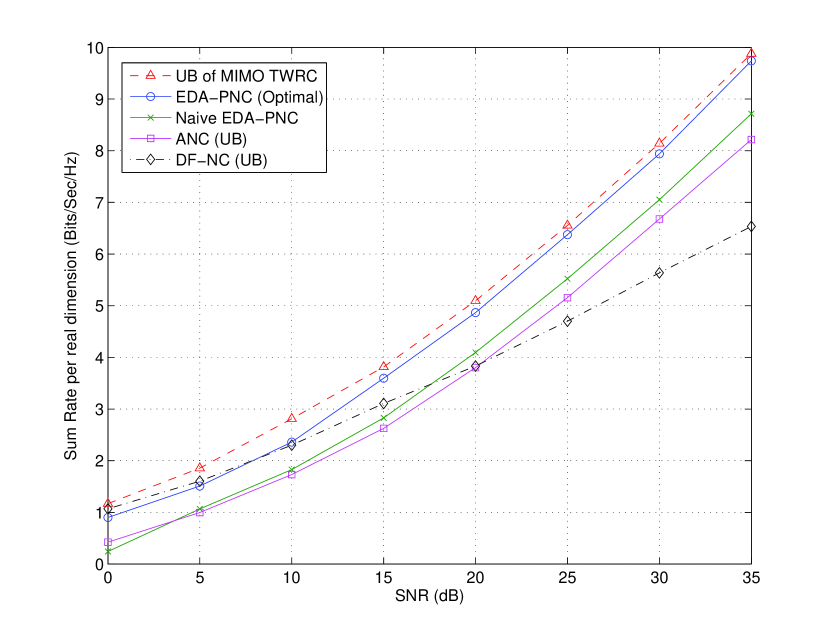
Figure 3: Achievable sum-rate of the proposed EDA-PNC scheme for a MIMO TWRC with $n_{T}=n_{R}=2.$

Here, we present the numerical results for real-valued MIMO TWRCs with $n_{T}=n_{R}=2$. The coefficients in the channel matrices are independently drawn from $\mathcal{N}(0,1)$. The optimal rotation matrix $\mathbf{K}$ and the optimal power matrices $\mathbf{\Psi}_{A}$ and $\mathbf{\Psi}_{B}$ are found by utilizing the exhaustive search method. The achievable sum-rate of the proposed EDA-PNC scheme is plotted in Fig. 3. The sum-capacity UB of the MIMO TWRC, the achievable sum-rate UBs of the ANC and DF-NC schemes, as well as the achievable sum-rate of the naive EDA-PNC (with $\mathbf{K=I}$) scheme, are also included for comparison. In the high SNR region, we observe that the gap between the achievable sum-rate of the proposed EDA-PNC scheme and the sum-capacity UB of the MIMO TWRC is very small, e.g., less than 0.3 bit/Sec/Hz in spectral efficiency, or less than 0.4 dB in power efficiency, at a SNR greater than 15 dB. We also see that the proposed EDA-PNC scheme significantly outperforms the ANC, DF-NC and the naive EDA scheme. Specifically, the ANC scheme suffers from a significant power loss of about 3-4 dB compared with the proposed EDA-PNC scheme. The DF-NC scheme suffers from a severe multiplexing loss, as the slope of its performance curve is nearly halved compared to the other schemes. In the low SNR region, we observe that the DF-NC scheme almost achieves the sum-capacity UB, and that the proposed EDA-PNC scheme is inferior to the DF-NC scheme. This is due to the inherited disadvantage of nested lattice codes in the low SNR region [2].

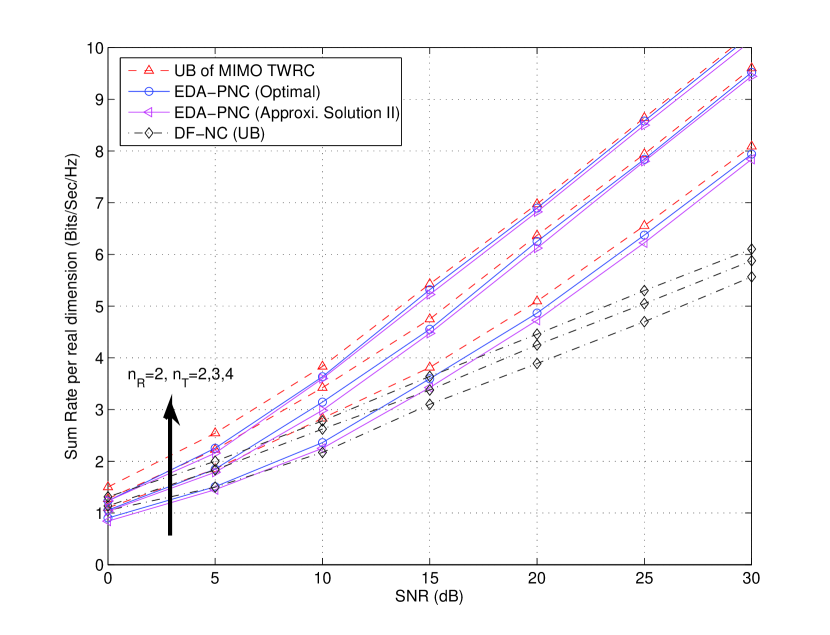
Figure 4: Achievable sum-rate of the proposed EDA-PNC scheme for MIMO TWRCs with $n_{R}=2$, $n_{T}=2,3,4$.

Next, we show the numerical result of the proposed EDA-PNC scheme for MIMO TWRCs with $n_{R}=2$ and $n_{T}=2,3,4$. In Fig. 4, two performance curves of the proposed EDA-PNC scheme are illustrated. One is based on the exhaustive search method, and the other is based on the approximate solution II (AS-II) method developed in Section VI. The sum-capacity UBs of the MIMO TWRCs and the performance curves of the DF-NC scheme are also plotted. In the medium-to-high SNR region, the gap between the proposed EDA-PNC scheme and the sum-capacity UB of the MIMO TWRC diminishes as $n_{T}$ increases. This agrees well with the asymptotic optimality of EDA-PNC, as stated in Theorem 2. We also see that there is a tiny gap between the optimal EDA-PNC curve (obtained from the exhaustive search) and the one based on AS-II. This implies that the proposed AS-II algorithm is nearly optimal for $n_{R}$ $=2$.

VII-B Achievable Rates of MIMO TWRCs with $n_{T}\geq n_{R}=4$

Now, we consider complex-valued MIMO TWRCs with $n_{T}\geq n_{R}=4$. The channel coefficients are now independently drawn from $\mathcal{CN}$(0,1). In this case, the complexity of exhaustive search in finding the the optimal EDA precoder is prohibitively high. Thus, we confine our results to the approximate solutions developed in Section VI.

VII-B1 Achievable Sum-Rates

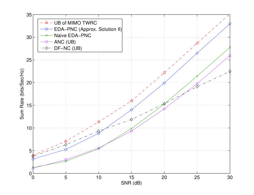
Figure 5: Achievable sum-rate of the proposed EDA-PNC scheme for a MIMO TWRC with $n_{T}=n_{R}=4.$

In Fig. 5, we plot the achievable sum-rate of the proposed EDA-PNC scheme with $n_{T}=n_{R}=4$. This figure also includes the performance curves of the other schemes considered in Fig. 3. The only difference is that the AS-II algorithm is used in plotting the performance curve of the proposed EDA-PNC scheme. Comparing Fig. 5 with Fig. 3, we see that the relative performance trends of these schemes are quite similar, except that the gap between the proposed EDA-PNC and the capacity UB is slightly larger (about 1.4 dB in power efficiency in the high SNR region) in Fig. 5. We conjecture that this performance degradation is mainly due to the sub-optimality of AS-II. We will seek for the possibility of improving AS-II in our future work.

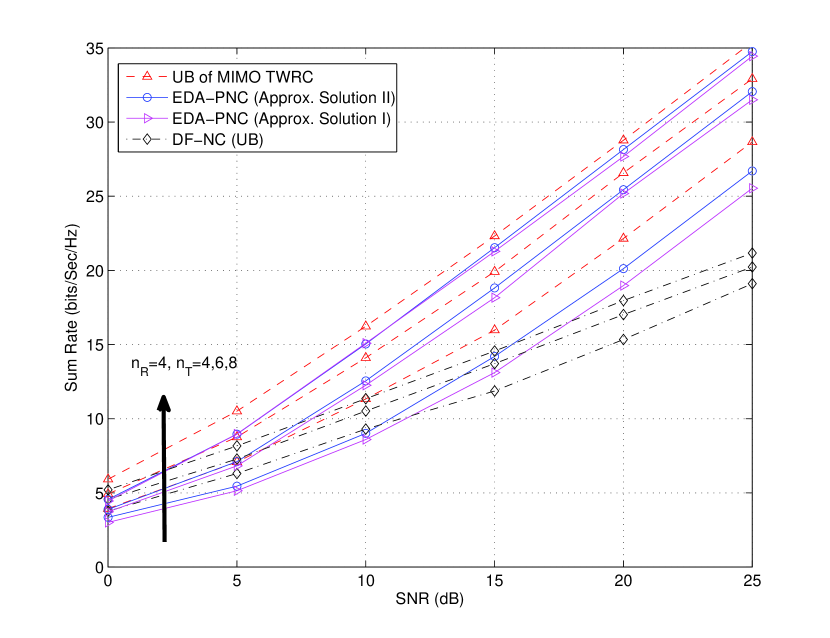
Figure 6: Achievable sum-rate of the proposed EDA-PNC scheme for MIMO TWRCs with $n_{R}=4$, $n_{T}=4,6,8$.

In Fig. 6, we further study the impact of $n_{T}$ on the achievable sum-rate in the case of $n_{R}$ $=4$. Similar to Fig. 4, we see that the proposed EDA-PNC scheme asymptotically approaches the capacity UB as $n_{T}$ increases. It is also worth mentioning that, for $n_{T}=8$ and $n_{R}=4$, the proposed EDA-PNC scheme can increase the spectral efficiency by more than 50% relative to the DF-NC scheme, at a practical SNR level (e.g., SNR=15 dB). In addition, we compare the performance of AS-I and AS-II algorithms in Fig. 6. We see that AS-II always slightly outperforms AS-I. For this reason, we only include the performance curves of AS-II in the other figures presented in this paper.

VII-B2 Achievable Rate-Regions

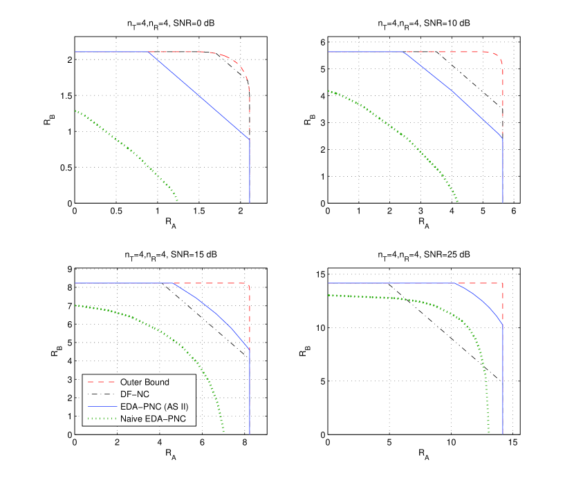
Figure 7: Achievable rate-region of the proposed EDA-PNC scheme for a MIMO TWRC with $n_{T}=n_{R}=4,$ where $SNR=0,10,15,25$ dB.

We next show the achievable rate-region of the proposed EDA-PNC scheme (based on AS-II). The results for the case of $n_{T}=n_{R}=4$ is shown in Fig. 7, at SNR = 0, 10, 15, 25 dB. We also include the rate-regions of the capacity UB, the DF-NC scheme and the naive EDA-PNC scheme. Clearly, the proposed scheme achieves a significantly larger rate-region relative to the DF-NC scheme and the naive EDA-PNC scheme, at a medium-to-high SNR. For a SNR of 15 dB, the proposed EDA-PNC scheme outperforms the DF-NC scheme, whereas the naive EDA-PNC scheme is worse than the DF-NC scheme, for the entire rate-region. Compared to the naive EDA precoding, the performance gain achieved by the proposed EDA precoding is significant. For low SNRs, e.g., SNR = 0 dB, the achievable rate-region of DF-NC is very close to the capacity outer bound of the MIMO TWRC and is better than that of the EDA-PNC scheme. This is in agreement with the observations in Figs. 3-6.

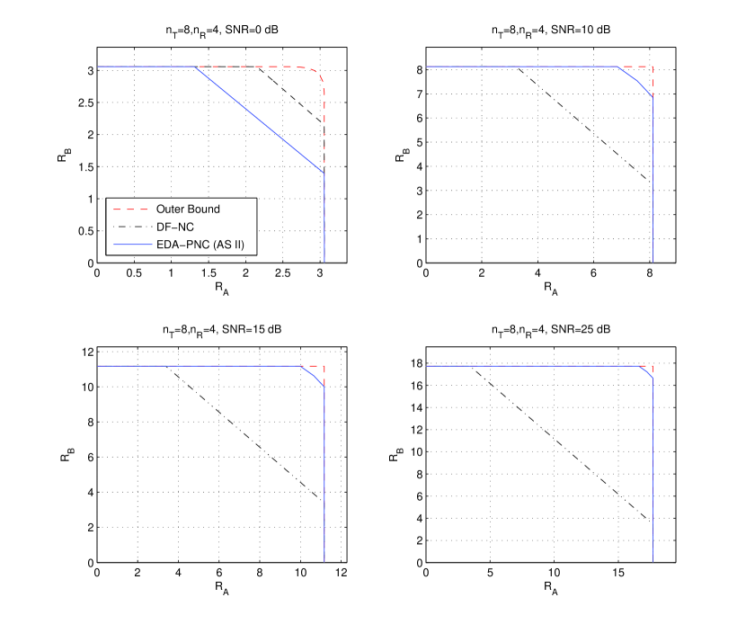
Figure 8: Achievable rate-region of the proposed EDA-PNC scheme for a MIMO TWRC with $n_{T}=8$, $n_{R}=4,$ where $SNR=0,10,15,25$ dB.

Finally, in Fig. 8, we plot the achievable rate-region of the proposed EDA-PNC scheme with $n_{T}=8$ and $n_{R}=4$. Comparing to Fig. 7, we observe that the gap between the achievable rate-region of the proposed EDA-PNC scheme and the capacity outer bound of MIMO TWRC becomes smaller for the entire SNR range. This agrees well with Theorem 2.

In summary, the results shown in Fig. 3-8 clearly demonstrates the benefits of the proposed EDA-PNC scheme for MIMO TWRCs.

VIII Conclusions

In this paper, we proposed an EDA-PNC scheme to approach the capacity of a MIMO TWRC. The proposed EDA precoder efficiently creates $n_{R}$ aligned parallel channels for the two users, which provides a platform to perform multi-stream PNC. In such a manner, the benefits of PNC can now be exploited in a MIMO two-way relay system. We derived an achievable rate of the proposed EDA-PNC scheme and showed that, as $n_{T}/n_{R}$ increases (towards infinity), the proposed EDA-PNC scheme approaches the capacity upper bound of a MIMO TWRC. For a finite $n_{T}$, numerical results demonstrated that there is only a marginal gap between the achievable rate of the proposed scheme and the capacity upper bound, and the proposed scheme clearly outperforms the existing benchmark schemes. It is worth mentioning that the discussions in this paper is limited to the situation of $n_{T}\geq n_{R}$. The extension of this work to the case of $n_{T}<n_{R}$ requires a dimension reduction method and is of interest for future work.

Appendix I Treatment for a Complex-Valued Model

The results of this paper derived based on a real-valued system model can be readily extended to the case of a complex-valued model. The key observation is that every complex-valued system model can be equivalently expressed in a real-valued form.

For example, suppose that the uplink channel model in (1) is complex-valued. It can be equivalently expressed in a real-valued form as

$$\left[\begin{array}[]{c}\mathfrak{R}\left(Y_{R}\right)\\ \mathfrak{I}\left(Y_{R}\right)\end{array}\right]=\sum\limits_{m\in\left\{A,B\right\}}\left[\begin{array}[]{cc}\mathfrak{R}\left(\mathbf{H}_{m,R}\right)&-\mathfrak{I}\left(\mathbf{H}_{m,R}\right)\\ \mathfrak{I}\left(\mathbf{H}_{m,R}\right)&\mathfrak{R}\left(\mathbf{H}_{m,R}\right)\end{array}\right]\left[\begin{array}[]{c}\mathfrak{R}\left(X_{m}\right)\\ \mathfrak{I}\left(X_{m}\right)\end{array}\right]+\left[\begin{array}[]{c}\mathfrak{R}\left(Z_{R}\right)\\ \mathfrak{I}\left(Z_{R}\right)\end{array}\right]$$ (43)

where $\mathfrak{R}\left(\mathbf{\cdot}\right)$ and $\mathfrak{I}\left(\mathbf{\cdot}\right)$ denote the real part and imaginary part of a complex-valued matrix (or a vector), respectively.

It is noteworthy that the above relationship also applies to the downlink channel model (6). In this way, the results obtained for the real-valued system are directly applicable to a complex-valued system.

Appendix II Proof of Theorem 1

Here we only provide a sketch of the proof. We refer the interested readers to [2] (cf., proof of Th.1 in [2]) for more details.

VIII-A Uplink Achievable Rate-Pair

Recall from (16) that the $n_{R}$ aligned eigen-modes (sub-channels) created by EDA precoding can be written in an entry-by-entry form as

$$y_{R,i}\left[l\right]=\Psi_{A}\left(i,i\right)c_{A,i}\left[l\right]+\Psi_{B}\left(i,i\right)c_{B,i}\left[l\right]+z_{R,i}\left[l\right],l=1,\cdots,n,i=1,\cdots,n_{R}.$$ (44)

where $y_{n_{R},i}\left[l\right]$ (or $z_{n_{R},i}\left[l\right]$) represents the $i$th entry of $\widetilde{Y}_{R}\left[l\right]$ (or $\widetilde{Z}_{R}\left[l\right]$).

VIII-A1 Encoding

The construction of nested lattice codes for each sub-channel $i$ follows exactly from [2]. Let $\mathcal{C}_{m,i}$, $m\in\left\{A,B\right\}$, be the codebook of user $m$ for the $i$th sub-channel, and 2${}^{nR_{m,i}}$ be the size of $\mathcal{C}_{m,i}$. To deliver a message in the $i$th sub-channel, user $m$ chooses a codeword $W_{m,i}\in\mathcal{C}_{m,i}$ associated with the message. After a random dithering and a module-lattice operation [2], a length-$n$ signal sequence

$$\mathbf{c}_{m,i}=\left[c_{m,i}\left[1\right],\cdots,c_{m,i}\left[n\right]\right],$$

is generated which will be transmitted in the $i$th sub-channel. The above encoding operation is performed for all $n_{R}$ sub-channels.

VIII-A2 Decoding (the bin-index) at the Relay

Upon receiving $\left\{\widetilde{Y}_{R}\left[l\right]\right\}_{l=1}^{n}$, the relay computes the so-called “bin-index” $T_{i}$ instead of $W_{A,i}$ and $W_{B,i}$ for each sub-channel $i$, $i=1,\cdots,n_{R}$. (See the definition of bin-index in [2]). From Theorem 3 in [2], the error probability of recovering the bin-index $T_{i}$ at the relay is arbitrarily small as $n\rightarrow\infty$ if

$$R_{A,i} \leq \frac{1}{2}\left[\log\left(\frac{\Psi_{A}\left(i,i\right)^{2}}{\Psi_{A}\left(i,i\right)^{2}+\Psi_{B}\left(i,i\right)^{2}}+\Psi_{A}\left(i,i\right)^{2}\right)\right]^{+},\text{ }$$ (45a)

$$R_{B,i} \leq \frac{1}{2}\left[\log\left(\frac{\Psi_{B}\left(i,i\right)^{2}}{\Psi_{A}\left(i,i\right)^{2}+\Psi_{B}\left(i,i\right)^{2}}+\Psi_{B}\left(i,i\right)^{2}\right)\right]^{+},$$ (45b)

where $i=1,\cdots,n_{R}.$

Since the aligned sub-channels are orthogonal to each other, the rate-pair ($R_{A}$, $R_{B}$) with which all the bin-indices $\left\{T_{i}\right\}_{i=1}^{n_{R}}$ can be recovered correctly is given by (19a) and (19b).

VIII-B Downlink Achievable Rate-Pair

VIII-B1 Relay’s Encoding

Define a “super bin-index” as $T$ $\mathbf{\triangleq[}T_{1},T_{2},\cdots,T_{n_{R}}\mathbf{]}$ and assume that $T$ is recovered correctly by the relay. Also, assume that $R_{A}\geq R_{B}$. We generate 2${}^{nR_{A}}$ $n_{R}$-by-$n$ codeword matrices with each column drawn independently from a multi-variant Gaussian distribution with zero mean and covariance $\mathbf{Q}_{R}$. This forms a rate-$R_{A}$ codebook $\mathcal{C}_{R}$ (whose generation is independent of the codebooks $\left\{\mathcal{C}_{m,1},\cdots,\mathcal{C}_{m,n_{R}}\right\}$ used in the uplink phase). The codebook $\mathcal{C}_{R}$ is employed to map each super bin-index $T$ into a codeword in $\mathcal{C}_{R}$. Denote by $\mathbf{X}_{R}\left(T\right)$ the codeword in $\mathcal{C}_{R}$ mapped to $T$. Then, $\mathbf{X}_{R}\left(T\right)$ is transmitted over the $n_{R}$ antennas at the relay.

VIII-B2 Decoding of the Two Users

Upon receiving $\mathbf{Y}_{A}$, user $A$ decodes $T_{A}$, by finding in $\mathcal{C}_{A}^{DL}$ a codeword that is jointly typical with $\mathbf{Y}_{A}$. Here, $\mathcal{C}_{A}^{DL}$ is constructed by selecting the codewords in $\mathcal{C}_{R}$ corresponding to $\left[W_{A,1},\cdots,W_{A,n_{R}}\right]$ (which are perfectly known to user $A)$. Note that the cardinality of $\mathcal{C}_{A}^{DL}$ is $2^{nR_{B}}$ [2]. From the argument of random coding and jointly typical decoding [11], we have $\Pr\left[T_{A}\neq T\right]\rightarrow 0$ as $n\rightarrow\infty$ if

$$R_{B}\leq R_{B,DL}^{EDA}=\frac{1}{2}\log\det\left(\mathbf{I}+\mathbf{H}_{R,A}\mathbf{Q}_{R}\mathbf{H}_{R,A}^{T}\right).$$ (46a)

With $$T=\left[T_{1},\cdots,T_{n_{R}}\right] \left[W_{A,1},\cdots,W_{A,n_{R}}\right] A B$$ and , user can uniquely determine the messages of user using the method described in [2].

Similarly, user $B$ can reliably determine the messages of user A if

$$R_{A}\leq R_{A,DL}^{EDA}=\frac{1}{2}\log\det\left(\mathbf{I}+\mathbf{H}_{R,B}\mathbf{Q}_{R}\mathbf{H}_{R,B}^{T}\right).$$ (46b)

Combining (19a), (19b), (46a) and (46b), we complete the proof of Theorem 1.

Appendix III Proof of Theorem 2

Proof:

Since the downlink rate-pair of the EDA-PNC scheme is identical to that of the capacity UB, we only need to consider the uplink rate-pair. Specifically, we need to show that

$$R_{m,UL}^{UB}-R_{m,UL}^{EDA}\overset{\text{P}}{\rightarrow}0\text{ for }n_{T}\rightarrow\infty\text{, }m\in\left\{A,B\right\}\text{.}$$ (47)

Clearly, $R_{m,UL}^{UB}$ and $R_{m,UL}^{EDA}$ are continuous functions of $\mathbf{H}_{m,R}\mathbf{H}_{m,R}^{T}$. From the property of convergence in probability (cf., Theorem 4, pp. 261 of [30]), to prove (47), it suffices to show that, if

$$\frac{1}{n_{T}}\mathbf{H}_{m,R}\mathbf{H}_{m,R}^{T}\rightarrow\mathbf{I}\text{, as }n_{T}\rightarrow\mathbf{\infty,}$$ (48)

then

$$R_{m,UL}^{UB}-R_{m,UL}^{EDA}\rightarrow 0\text{, for }n_{T}\rightarrow\infty.$$ (49)

From (7a) and (7b), we have

$$R_{m,UL}^{UB}=\frac{1}{2}\log\det\left(\mathbf{I}+\mathbf{H}_{m,R}\mathbf{Q}_{m}\mathbf{H}_{m,R}^{T}\right).$$ (50)

Let $P_{m,T}$ be the power allocated to user $m$, $m\in\left\{A,B\right\}$. With (48), it can be shown that as $n_{T}\rightarrow\mathbf{\infty}$, the optimal $\mathbf{Q}_{m}$ takes the form of

$$\mathbf{Q}_{m}=\frac{P_{m,T}}{n_{R}n_{T}}\mathbf{H}_{m,R}^{T}\mathbf{H}_{m,R}.$$ (51)

Thus, as $n_{T}\rightarrow\mathbf{\infty}$, we obtain

$$R_{m,UL}^{UB} = \frac{1}{2}\log\det\left(\mathbf{I+}\frac{P_{m,T}}{n_{R}n_{T}}\mathbf{H}_{m,R}\mathbf{H}_{m,R}^{T}\mathbf{H}_{m,R}\mathbf{H}_{m,R}^{T}\right)$$

$$= \frac{1}{2}n_{R}\log n_{T}+\frac{1}{2}\log\det\left[\frac{1}{n_{T}}\mathbf{I+}\frac{P_{m,T}}{n_{R}}\left(\frac{1}{n_{T}}\mathbf{H}_{m,R}\mathbf{H}_{m,R}^{T}\right)\left(\frac{1}{n_{T}}\mathbf{H}_{m,R}\mathbf{H}_{m,R}^{T}\right)\right]$$

$$= \frac{1}{2}n_{R}\log n_{T}+\frac{1}{2}\log\det\left[\frac{P_{m,T}}{n_{R}}\mathbf{I}\right]+o\left(1\right)$$ (52b)

$$= \frac{n_{R}}{2}\log\left(\frac{n_{T}P_{m,T}}{n_{R}}\right)+o\left(1\right),$$ (52c)

where (52) follows by substituting (51) into (50), and (52b) follows from (48).

Now, consider the EDA precoder

$$\mathbf{F}_{m}=\mathbf{H}_{m,R}^{T}\left(\mathbf{H}_{m,R}\mathbf{H}_{m,R}^{T}\right)^{-1}\mathbf{K\Psi}_{m}\,\text{, }m\in\left\{A,B\right\}\text{.}$$ (53)

We choose

$$\mathbf{K=I}\text{ and }\mathbf{\Psi}_{m}=\sqrt{\frac{n_{T}P_{m,T}}{n_{R}}}\mathbf{I}.$$ (54)

The power constraint is asymptotically met, i.e.,

$$\text{Tr}\left\{\mathbf{F}_{m}\mathbf{F}_{m}^{T}\right\}=\text{Tr}\left\{\left(\mathbf{H}_{m,R}\mathbf{H}_{m,R}^{T}\right)^{-1}\frac{n_{T}P_{m,T}}{n_{R}}\right\}\overset{\text{P}}{\rightarrow}P_{m,T}\text{, for }n_{T}\rightarrow\infty.$$ (55)

The choice of $\mathbf{K}$ and $\mathbf{\Psi}_{m}$ in (54) is in no sense optimal. However, we will show that this suboptimal choice is sufficient to prove (49). To see this, the uplink achievable rate of the EDA-PNC scheme is given by

$$R_{m,UL}^{EDA} = \frac{1}{2}\sum_{i=1}^{n_{R}}\left[\log\left(\frac{\Psi_{m}^{2}\left(i,i\right)}{\Psi_{A}^{2}\left(i,i\right)+\Psi_{B}^{2}\left(i,i\right)}+\Psi_{m}^{2}\left(i,i\right)\right)\right]^{+}$$ (56)

$$= \frac{n_{R}}{2}\log\left(\frac{n_{T}P_{m,T}}{n_{R}}\right)+o(1)\text{, as }n_{T}\rightarrow\infty,$$ (57)

where (56) follows from Theorem 2 and (57) is from (54) together with the fact that $\frac{\Psi_{m}^{2}\left(i,i\right)}{\Psi_{A}^{2}\left(i,i\right)+\Psi_{B}^{2}\left(i,i\right)}\leq 1$, for $i=1,\cdots,n_{R}$.

Combining (52c) and (57), we arrive at (49), which completes the proof of Theorem 2.    

Appendix IV Proof of Lemma 3

Proof:

The objective function (37) is jointly concave in $\left\{\Sigma\left(1,1\right),\cdots,\Sigma\left(n_{R},n_{R}\right)\right\}$. The Lagrangian of problem (37) is given by

$$L\left(\lambda,\Sigma\left(1,1\right),\cdots,\Sigma\left(n_{R},n_{R}\right)\right)$$ (58)

$$= \frac{\alpha}{2}\mathop{\displaystyle\sum}\limits_{i\in S_{A}}\left[\log\left(\frac{1}{1+\gamma^{2}}+\Sigma\left(i,i\right)^{2}\right)\right]+\frac{1-\alpha}{2}\mathop{\displaystyle\sum}\limits_{i\in S_{B}}\left[\log\left(\frac{\gamma^{2}}{1+\gamma^{2}}+\gamma^{2}\Sigma\left(i,i\right)^{2}\right)\right]$$

$$-\lambda\mathop{\displaystyle\sum}\limits_{i=1}^{k}\Lambda_{G\left(\gamma\right)}\left(i,i\right)\Sigma\left(i,i\right)^{2}$$

where $\lambda$ is a non-negative scalar. The partial derivative of the Lagrangian in (58) with respect to each $\Sigma\left(i,i\right)^{2}$ is given by

$$\frac{\partial L}{\partial\left(\Sigma\left(i,i\right)^{2}\right)}=\left\{\begin{array}[]{cc}\frac{1}{2}\frac{1}{\frac{1}{1+\gamma^{2}}+\Sigma\left(i,i\right)^{2}}-\lambda\Lambda_{G\left(\gamma\right)}\left(i,i\right),&\text{if }i\in S_{A}\text{ and }i\in S_{B}\\ \frac{1}{2}\frac{\alpha}{\frac{1}{1+\gamma^{2}}+\Sigma\left(i,i\right)^{2}}-\lambda\Lambda_{G\left(\gamma\right)}\left(i,i\right),&\text{if }i\in S_{A}\text{ and }i\notin S_{B}\\ \frac{1}{2}\frac{1-\alpha}{\frac{1}{1+\gamma^{2}}+\Sigma\left(i,i\right)^{2}}-\lambda\Lambda_{G\left(\gamma\right)}\left(i,i\right),&\text{if }i\notin S_{A}\text{ and }i\in S_{B}\\ 0,&\text{if }i\notin S_{A}\text{ and }i\notin S_{B}\end{array}\right.$$

where $i=1,..,n_{R}.$ The Karush-Kuhn-Tucker condition is

$$\frac{\partial L}{\partial\left(\Sigma\left(i,i\right)^{2}\right)}\left\{\begin{array}[]{c}=0,\text{ if }\Sigma\left(i,i\right)>0\\ \leq 0,\text{ if }\Sigma\left(i,i\right)=0\end{array}\right.$$ (59)

which yields the solution (38).    

Appendix V Proof of Lemma 4

Without loss of generality, let the SVD of $\mathbf{K\Sigma}$ be

$$\mathbf{K\Sigma}=\mathbf{UDV}^{T}.$$ (60)

where the diagonal elements of $\mathbf{\Sigma}$ and $\mathbf{D}$ are both arranged in the descending order. From (60), the rank of $\mathbf{D}$ is the same as $\mathbf{\Sigma}$ (as $\mathbf{K}$, $\mathbf{U}$, and $\mathbf{V}$ are all of full rank). This implies that, if $\Sigma\left(i,i\right)$ $=0$ for any index $i$, then $D\left(i,i\right)$ $=0$.

Let us first consider that $\mathbf{\Sigma}$ has full rank. We will relax this constraint later. Using (32), we obtain

$$\text{Tr}(\mathbf{G}(\gamma)\mathbf{UD}^{2}\mathbf{U}^{T})=\text{Tr}\left(\mathbf{U}_{G\left(\gamma\right)}\mathbf{\Lambda}_{G\left(\gamma\right)}\mathbf{U}_{G\left(\gamma\right)}^{T}\mathbf{UD}^{2}\mathbf{U}^{T}\right)\geq\text{Tr}\left(\mathbf{\Lambda}_{G\left(\gamma\right)}\cdot\mathbf{D}^{2}\right)$$

where the diagonal entries of $\mathbf{\Lambda}_{G\left(\gamma\right)}$ are arranged in the ascending order, and the equality holds when $\mathbf{U}=\mathbf{U}_{G\left(\gamma\right)}$.

Then, the optimization problem in (41a) and (41b) can be expressed as

$$\min_{\mathbf{D},\mathbf{V}}\text{Tr}\left(\mathbf{\Lambda}_{G\left(\gamma\right)}\cdot\mathbf{D}^{2}\right)$$ (61a)

s.t.

$$\left[\mathbf{VD}^{-2}\mathbf{V}^{T}\right]_{\text{diag}}=\mathbf{\Sigma}^{-2}.$$ (61b)

Note that the diagonal elements of $\mathbf{\Sigma}^{-2}$ and $\mathbf{D}^{-2}$ are both arranged in the ascending order. Denote the diagonal entries of $\mathbf{\Sigma}^{-2}$ by $\left[\sigma_{1},\cdots\sigma_{n_{R}}\right]$ and those of $\mathbf{D}^{-2}$ as $\left[d_{1},\cdots,d_{n_{R}}\right]$. From Th. 4.3.32 of [32], for any $\left[d_{1},\cdots,d_{n_{R}}\right]$ majorized by $\left[\sigma_{1},\cdots\sigma_{n_{R}}\right]$, there always exists a unitary matrix $\mathbf{V}$ satisfying (61b).  Therefore, the optimization problem specified in (61a) and (61b) becomes

$$\min_{d_{1},\cdots,d_{n_{R}}}\sum_{i=1}^{n_{R}}\frac{\Lambda_{G\left(\gamma\right)}\left(i,i\right)}{d_{i}}$$ (62)

subject to the majorization constraint as [32]

$$d_{i} \geq 0\text{ }\forall\text{ }i\in\left\{1,\cdots,n_{R}\right\}$$ (63)

$$d_{1} \leq d_{2}\leq\cdots\leq d_{n_{R}}$$

$$\sum_{i=1}^{t}d_{i} \leq \sum_{i=1}^{t}\sigma_{i},t=1,\cdots,n_{R}-1,$$

$$\sum_{i=1}^{n_{R}}d_{i} = \sum_{i=1}^{n_{R}}\sigma_{i}.$$

We next show that, with $\mathbf{\Sigma}$ given by (40), the solution to the optimization problem (41a) (41b) is given by

$$d_{i}=\sigma_{i},\forall\text{ }i=1,...,n_{R}.$$ (64)

To prove (64), we need some facts, as detailed below.

Fact 2

For any $i,j\in\left\{1,\cdots,n_{R}\right\}$ with $i<j$, we have

$$\frac{\Lambda_{G}\left(i,i\right)}{\sigma_{i}^{2}}\geq\frac{\Lambda_{G}\left(j,j\right)}{\sigma_{j}^{2}}.$$ (65)

Proof:

From (40), we have

$$\sigma_{i}=\frac{1}{\left[\left(\frac{1}{2\lambda\Lambda_{G\left(\gamma\right)}\left(i,i\right)}-\frac{1}{1+\gamma^{2}}\right)^{+}\right]}$$ (66)

where $\lambda>0$. Note that $\sigma_{i}>0$ for all $i=1,...,n_{R}$ (as $\mathbf{\Sigma}$ is of full rank). Then,

$$\frac{\sigma_{i}^{2}}{\sigma_{j}^{2}}=\frac{\left(\frac{1}{2\lambda\Lambda_{G\left(\gamma\right)}\left(j,j\right)}-\frac{1}{1+\gamma^{2}}\right)^{2}}{\left(\frac{1}{2\lambda\Lambda_{G\left(\gamma\right)}\left(i,i\right)}-\frac{1}{1+\gamma^{2}}\right)^{2}}\overset{\left(1\right)}{\leq}\frac{\left(\frac{1}{2\lambda\Lambda_{G\left(\gamma\right)}\left(j,j\right)}\right)^{2}}{\left(\frac{1}{2\lambda\Lambda_{G\left(\gamma\right)}\left(i,i\right)}\right)^{2}}\overset{\left(2\right)}{\leq}\frac{\frac{1}{2\lambda\Lambda_{G\left(\gamma\right)}\left(j,j\right)}}{\frac{1}{2\lambda\Lambda_{G\left(\gamma\right)}\left(i,i\right)}}=\frac{\Lambda_{G\left(\gamma\right)}\left(i,i\right)}{\Lambda_{G\left(\gamma\right)}\left(j,j\right)},$$ (67)

where steps $\overset{\left(1\right)}{\leq}$ and $\overset{\left(2\right)}{\leq}$ are both from $\frac{1}{2\lambda\Lambda_{G\left(\gamma\right)}\left(j,j\right)}\leq\frac{1}{2\lambda\Lambda_{G\left(\gamma\right)}\left(i,i\right)}$ (as the diagonal elements of $\Lambda$_G(γ) are arranged in the ascending order). This yields (65).    

From (63), we see that, for any $\left[d_{1},\cdots,d_{n_{R}}\right]$ in the feasible region, $d_{1}\leq\sigma_{1}$ and $d_{n_{R}}\geq\sigma_{n_{R}}$. Denote the objective function in (62) as

$$f\left(d_{1},\cdots,d_{n_{R}}\right)=\mathop{\displaystyle\sum}\limits_{i=1}^{n_{R}}\frac{\Lambda_{G\left(\gamma\right)}\left(i,i\right)}{d_{i}}.$$ (68)

For any $d_{1}\leq\sigma_{1}$ and $d_{n_{R}}\geq\sigma_{n_{R}}$, let $\varepsilon$ be a non-negative number satisfying

$$d_{1}+\varepsilon\leq\sigma_{1}\text{ and }d_{n_{R}}-\varepsilon\geq\sigma_{n_{R}}.$$ (69)

Fact 3

$$f\left(d_{1}+\varepsilon,\cdots,d_{n_{R}}-\varepsilon\right)\leq f\left(d_{1},\cdots,d_{n_{R}}\right)$$ (70)

where equality holds when $\varepsilon=0$.

Proof:

We have

$$f\left(d_{1}+\varepsilon,\cdots,d_{n_{R}}-\varepsilon\right)-f\left(d_{1},\cdots,d_{n_{R}}\right)$$

$$=\frac{\Lambda_{G\left(\gamma\right)}\left(1,1\right)}{d_{1}+\varepsilon}+\frac{\Lambda_{G\left(\gamma\right)}\left(n_{R},n_{R}\right)}{d_{n_{R}}-\varepsilon}-\left(\frac{\Lambda_{G\left(\gamma\right)}\left(1,1\right)}{d_{1}}+\frac{\Lambda_{G\left(\gamma\right)}\left(n_{R},n_{R}\right)}{d_{n_{R}}}\right)$$

$$=-\Lambda_{G\left(\gamma\right)}\left(1,1\right)\frac{\varepsilon}{\left(d_{1}+\varepsilon\right)d_{1}}+\Lambda_{G\left(\gamma\right)}\left(n_{R},n_{R}\right)\frac{\varepsilon}{\left(d_{n_{R}}-\varepsilon\right)d_{n_{R}}}$$

$$\overset{(a)}{\leq}-\Lambda_{G\left(\gamma\right)}\left(1,1\right)\frac{\varepsilon}{\left(d_{1}+\varepsilon\right)^{2}}+\Lambda_{G\left(\gamma\right)}\left(n_{R},n_{R}\right)\frac{\varepsilon}{\left(d_{n_{R}}-\varepsilon\right)^{2}}$$

$$=\left(-\frac{\Lambda_{G\left(\gamma\right)}\left(1,1\right)}{\left(d_{1}+\varepsilon\right)^{2}}+\frac{\Lambda_{G\left(\gamma\right)}\left(n_{R},n_{R}\right)}{\left(d_{n_{R}}-\varepsilon\right)^{2}}\right)\varepsilon$$

$$\overset{(b)}{\leq}\left(-\frac{\Lambda_{G\left(\gamma\right)}\left(1,1\right)}{\sigma_{1}^{2}}+\frac{\Lambda_{G\left(\gamma\right)}\left(n_{R},n_{R}\right)}{\sigma_{n_{R}}^{2}}\right)\varepsilon$$

$$\overset{(c)}{\leq}0$$

where step ($a$) is self-evident, step ($b$) follows from (69) and step ($c$) follows from (65) in Fact 1. The equalities in steps ($a$)-($c$) hold when $\varepsilon=0$, which completes the proof.    

Fact 3 implies that the objective function $f\left(d_{1}+\varepsilon,\cdots,d_{n_{R}}-\varepsilon\right),$ with $\varepsilon$ constrained by (69), is minimized when $\varepsilon=\sigma_{1}-d_{1}$ or $\varepsilon=\sigma_{n_{R}}-d_{n_{R}}$. Therefore, the optimum of the problem in (62) is achieved at either $d_{1}=\sigma_{1}$ or $d_{n_{R}}=\sigma_{n_{R}}$. Without loss of generality, we assume that $d_{1}=\sigma_{1}$. Then, the dimension of the problem in (62) reduces from $n_{R}$ to $n_{R}-1$. Applying the same reasoning to this ($n_{R}-1$)-dimension problem, we can further show that $d_{2}=\sigma_{2}$. Continuing this process, we eventually have (64), or equivalently,

$$\mathbf{D}=\mathbf{\Sigma}.$$

Therefore, from (60) and the uniqueness of SVD, we obtain $\mathbf{V}=\mathbf{I}$ and $\widetilde{\mathbf{K}}_{opt}^{\left(\gamma\right)}\mathbf{=U}_{G\left(\gamma\right)}=\mathbf{K}_{opt}^{(\gamma)}.$

Next, consider that $\mathbf{\Sigma}$ does not have full rank. Define

$$\overline{\mathbf{\Sigma}}=\mathbf{\Sigma}+\delta\sqrt{\mathbf{\Delta}}$$

where $\delta$ is an arbitrary positive number, and $\mathbf{\Delta}$ is a diagonal matrix with non-negative diagonal elements. We can properly choose such a $\mathbf{\Delta}$ that: (a) $\overline{\mathbf{\Sigma}}$ is of full rank; (b) For a sufficiently small $\delta$, Fact 2 always holds for $\overline{\mathbf{\Sigma}}$ (and so does Fact 3). To this end, we choose

$$\Delta\left(i,i\right)=0\text{, if }\Sigma\left(i,i\right)\neq 0$$ (71)

and

$$\frac{\Lambda_{G}\left(i,i\right)}{\Delta^{-2}\left(i,i\right)}\geq\frac{\Lambda_{G}\left(j,j\right)}{\Delta^{-2}\left(j,j\right)}\text{, if }\Sigma\left(i,i\right)=\Sigma\left(j,j\right)=0,i<j\text{.}$$ (72)

We verify Fact 2 for the above choice of $\mathbf{\Delta}$. Noting that the diagonal entries of $\mathbf{\Sigma}$ are arranged in descending order, we only need to consider three cases: (i) $\Sigma\left(i,i\right)$ $>$ 0, $\Sigma\left(j,j\right)$ $>$ 0, $i<j$; (ii) $\Sigma\left(i,i\right)$ $>$ 0, $\Sigma\left(j,j\right)$ = 0, $i<j$; (iii) $\Sigma\left(i,i\right)$ = $\Sigma\left(j,j\right)$ = 0, $i<j$. From our previous proof, Fact 2 holds for case (i). For case (ii), Fact 2 can be guaranteed by letting $\delta$ be sufficiently small. For case (iii), Fact 2 is guaranteed from (72). Thus, Fact 2 is guaranteed for a sufficiently small $\delta$ and the chosen $\mathbf{\Delta}$.

Now, consider the following optimization problem:

$$\min_{\mathbf{K}}\text{Tr}\left(\mathbf{G}\left(\gamma\right)\mathbf{K}\overline{\mathbf{\Sigma}}\mathbf{K}^{T}\right)$$ (73a)

s.t.

$$\left[\mathbf{K}^{-1}\left(\mathbf{K}^{-1}\right)^{T}\right]_{\text{diag}}=\mathbf{I}\text{.}$$ (73b)

Noting that $\overline{\mathbf{\Sigma}}$ is of full rank and Facts 2 and 3 hold for $\overline{\mathbf{\Sigma}}$, we see that the optimal solution to the above problem is $\mathbf{K}=\mathbf{K}_{opt}^{(\gamma)}$. Now, let $\delta\rightarrow 0$. From the continuity of the problem in (73), the optimal $\mathbf{K}$ is still given by $\mathbf{K}_{opt}^{(\gamma)}$. This completes the proof of Lemma 4.

References

- [1] S. Zhang, S. Liew, and P. Lam, “Physical-layer network coding,” in ACM Mobicom ‘06.
- [2] W. Nam, S. Chung, Y. H. Lee, “Capacity of the Gaussian two-way relay channel to within 1/2 bit”, IEEE Trans. Inform. Theory, vol. 56, no. 11, pp. 5488-5494, Nov. 2010.
- [3] M. P. Wilson, K. Narayanan, H. D. Pfister and A. Sprintson, “Joint physical layer coding and network coding for bidirectional relaying”, IEEE Trans. Inform. Theory, vol. 56, no. 11, pp. 5641-5654, Nov. 2010.
- [4] S. Katti, S. Gollakota, and D. Katabi, “Embracing Wireless Interference: Analog Network Coding”, ACM SIGCOMM’07.
- [5] R. Zhang, Y.-C. Liang, C. C. Chai, and S. Cui, “Optimal beamforming for two-way multi-antenna relay channel with analogue network coding,” IEEE Journal Select. Area. Comm., Vol. 27, No. 5, pp. 699-712, June 2009.
- [6] S. Xu and Y. Hua, “Source-relay optimization for a two-way MIMO relay system”, Proc. IEEE ICCASP 2010, pp. 3038-3041.
- [7] D. Gunduz, A. Goldsmith and H. V. Poor, “MIMO two-way relay channel: diversity-multiplexing tradeoff analysis”, Asilomar 2008.
- [8] G. Foschini, “Layered space-time architecture for wireless communication in a fading environment when using multi-element antennas,” Bell Labs Technical Journal, Autumn 1996, pp. 41-59.
- [9] R. Ahlswede, N. Cai, S.-Y. R. Li, and R. W. Yeung, “Network information flow,” IEEE Trans. Inform. Theory, vol. 46, pp. 1204–1216, Oct. 2000.
- [10] J. N. Laneman, D. N. C. Tse, and G. W. Wornell, “Cooperative diversity in wireless networks: Efficient protocols and outage behavior,” IEEE Trans. Inf. Theory, vol. 50, no. 12, pp. 3062–3080, Dec. 2004.
- [11] T. M. Cover and J. A. Thomas, Elements of Information Theory, New York: Wiley, 1991.
- [12] D. Tse and P. Visanath, Fundamentals of wireless communicationts, Cambridge University Press, 2006.
- [13] R. Zamir, S. Shamai and U. Erez, “Nested linear/lattice codes for structured multiterminal binning”, IEEE Trans. Inform. Theory, vol. 48, no. 6, pp. 1250-1276, June 2002.
- [14] U. Erez and R. Zamir, “Achieving 1/2 log(1 + SNR) on the AWGN channel with lattice encoding and decoding,” IEEE Trans. Inform. Theory, vol. 50, pp. 2293-2314, Oct. 2004.
- [15] R. A. Horn and C. R. Johnson, Matrix Analysis. Cambridge University Press, 1985.
- [16] T. Yang and X. Yuan, “Multi-stream physical layer network coding with Eigen-direction alignment precoding for MIMO two-way relay channels”, in preparation, 2011.
- [17] S. Zhang and S.-C. Liew, “Channel coding and decoding in a relay system operated with physical-layer network coding”, IEEE Journal Select. Area. Comm., vol. 27, no. 5, pp. 788-796, June 2009.
- [18] B. Nazer and M. Gastpar, “Computation over multiple-access channels,” IEEE Trans. Inform. Theory, vol. 53, pp. 3498–3516, Oct. 2007.
- [19] A. Goldsmith, “Wireless communicationts”, Cambridge University Press, 2005.
- [20] W. Yu, W. Rhee, S. Boyd and J. M. Cioffi, “Iterative water-filling for Gaussian vector multiple-access channels”, IEEE Trans. Inform. Theory, vol. 50, pp. 145–152, Jan. 2004.
- [21] X. Tang and Y. Hua, “Optimal design of non-regenerative MIMO wireless relays”, IEEE Trans. Wirele. Comm., vol. 6, pp. 1398–1407, Apr. 2007.
- [22] W. Nam, S.-Y. Chung and Y. H. Lee, “Nested latice codes for Gausian relay networks with interference”, submitted to IEEE Trans. Inform. Theory.
- [23] U. Erez, S. Litsyn and R. Zamir, “Lattices which are good for (almost) everything”, IEEE Trans. Inform. Theory, vol. 51, pp. 3401–3416, Oct. 2005.
- [24] G. D. Forney Jr., “On the role of MMSE estimation in approaching the information theoretic limits of linear Gaussian channels: Shannon meets wiener,” Proc. 41st Annual Allerton Conference, Oct. 2003.
- [25] T. E. Abrudan, J. Eriksson and V. Koivunen, “Steepest descent algorithms for optimization under unitary matrix constraint”, IEEE Trans. Sig. Proc., vol. 56, no. 3, pp. 1134-1147, Mar. 2008.
- [26] S. Boyd and L. Vandenberghe, “Convex optimization”, Cambridge University Press, 2004.
- [27] R. H. Y. Louie, Y. Li and B. Vucetic, “Practical physical layer network coding for two-way relay channels: performance analysis and comparison”, IEEE Trans. Wireless Comm., vol. 9, no. 2, pp. 764-777, Feb. 2010.
- [28] Q. F. Zhou, Y. Li, F. C. M. Lau and B. Vucetic, “Decode-and-forward two-way relaying with network coding and opportunistic relay selection”, IEEE Trans. Commun., vol. 58, no. 11, pp. 3070-3076, Nov. 2010.
- [29] T. Koike-Akino, P. Popovski and V. Tarokh, “Optimized constellations for two–way wireless relaying with physical network coding”, IEEE Jour. Select Area. Commun.., vol. 27, no. 5, pp. 773-787, June 2009.
- [30] V. K. Rohatgi and A. K. Md. E. Saleh, “An introduction to probability and statistics”, Wiley-Interscience, second edition, 2000.
- [31] Steven M. Kay, “Fundamentals of Statistical Signal Processing”, Prentice-Hall PTR, 1993.
- [32] R. A. Horn and C. R. Johnson, “Matrix Analysis”, Cambridge Unversity Press, 1990.
- [33] X. Yuan and T. Yang, “Near optimal precoding for a MIMO two-way relay system operated with analog network coding”, in preparation.