Smooth gauge for topological insulators

Abstract

We develop a technique for constructing Bloch-like functions for 2D $\mathbb{Z}_{2}$-insulators (i.e., quantum spin-Hall insulators) that are smooth functions of ${\bf k}$ on the entire Brillouin-zone torus. As the initial step, the occupied subspace of the insulator is decomposed into a direct sum of two “Chern bands,” i.e., topologically nontrivial subspaces with opposite Chern numbers. This decomposition remains robust independent of underlying symmetries or specific model features. Starting with the Chern bands obtained in this way, we construct a topologically nontrivial unitary transformation that rotates the occupied subspace into a direct sum of topologically trivial subspaces, thus facilitating a Wannier construction. The procedure is validated and illustrated by applying it to the Kane-Mele model.

I Introduction

In recent years the band theory of solids has been augmented by new chapters to account for geometric and topological effects that had not been considered previously. The introduction of the Berry phaseBerry-PRSL84 allowed the systematic description of many observable effects of purely geometric origin, such as the Aharonov-Bohm effect,Aharonov-PR59 and its applications in the band-theory context have included the theory of electric polarizationKing-Smith-PRB93 ; Resta-RMP94 and the anomalous Hall conductance.Thouless-PRL82 ; Haldane-PRL04

The recent discovery of topological insulatorsHasan-RMP10 ; Qi-RMP11 has widened the role of geometry and topology in band theory even further. The classification of non-interacting insulating Hamiltonians in 2D predicts two topologically nontrivial scenarios.Kitaev-AIP09 ; Schnyder-PRB08 ; Schnyder-AIP09 The first scenario is that of a Chern insulator, i.e., an insulator that exhibits an integer quantum Hall effect even in the absence of an external magnetic field.Haldane-PRL88 Such a material, also known as a quantum anomalous Hall insulator, is classified according to the value of transverse conductance in integer multiples of $e^{2}/h$, i.e., a $\mathbb{Z}$ classification. The $\mathbb{Z}$ invariant contains information about the excess chirality of current-carrying edge states of a 2D sample. Hamiltonians that correspond to different integers represent distinct topological phases, meaning that they cannot be adiabatically connected without closing the insulating gap.Kitaev-AIP09 ; Schnyder-PRB08 ; Schnyder-AIP09 Chern insulators break time-reversal (TR) symmetry, since $\sigma_{xy}$ is odd under TR. The name arises from the fact that the exact quantization of conductance is of topological origin, i.e., the conductance is written as $\sigma_{xy}=C(e^{2}/h)$ where $C$ is called the Chern number or TKNN invariant.Thouless-PRL82 ; Kohmoto-AP85 ; Nakahara-book

The second scenario in 2D is that of a TR-symmetric $\mathbb{Z}_{2}$ insulatorKane-PRL05-b that possesses either an odd or an even number of Kramers pairs of edge states. According to the number of these pairs at the edge, the insulator is either ${\mathbb{Z}_{2}}$-odd or ${\mathbb{Z}_{2}}$-even. These two phases are topologically distinct and cannot be adiabatically connected to one another without gap closure. A ${\mathbb{Z}_{2}}$-odd insulator realizes the quantum spin Hall (QSH)Kane-PRL05-b ; Kane-PRL05-a state, while a ${\mathbb{Z}_{2}}$-even one is adiabatically connected to a normal insulator. In what follows we sometimes refer to the QSH insulator as a “${\mathbb{Z}_{2}}$ insulator.” Unlike the Chern-insulator state, the QSH-insulator state has been realized experimentally, e.g., in CdTe/HgTe/CdTe quantum wellsKonig-Science07 following a theoretical prediction.Bernevig-Science06 ; Volkov-JETP85

On the level of conventional band theory of crystalline solids, Chern and ${\mathbb{Z}_{2}}$ insulators are also different from ordinary ones. For an ordinary insulator the Bloch states $\psi_{n{\bf k}}$ are usually assumed to be smooth and periodic in the Brillouin zone (BZ), meaning that a translation by a reciprocal lattice vector ${\bf G}$ returns the Bloch wavefunction back to itself with the same phase, $\psi_{n,{\bf k}+{\bf G}}=\psi_{n{\bf k}}$, and that $\psi$ is a smooth function of ${\bf k}$. Regarding the BZ as a torus, as in Fig. 1(a), this just means that $\psi$ is a smooth function of ${\bf k}$ on the torus. This turns out to be impossible for Chern insulators;Thouless-JPC84 ; Thonhauser-PRB06 the occupied space of a Chern insulator cannot be represented by smooth and periodic Bloch states. Usually periodicity is still assumed, in which case a point discontinuity or branch cut must appear in the phase of at least one occupied Bloch state somewhere in the BZ. It is now established that no gauge transformation – i.e., no ${\bf k}$-dependent unitary rotation of the bands in the occupied subspace – can smooth out this discontinuity.Thouless-JPC84 ; Thonhauser-PRB06

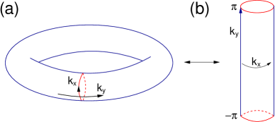
Figure 1: Brillouin zone in 2D represented as (a) a torus, and (b) a cylinder. We choose the gauge discontinuity to be distributed along the cross-sectional cut of the torus that maps onto the end loops of the cylinder at $k_{y}=\pm\pi$.

In the case of ${\mathbb{Z}_{2}}$ insulators, the presence of TR symmetry forces the total Chern number to vanish, guaranteeing the existence, in principle, of a smooth and periodic gauge in the BZ.Brouder-PRL07 However, it has been shown that any gauge that respects TR symmetry cannot be smooth on the torus for this class of topological materials.Fu-PRB06 ; Roy-PRB09-a ; Loring-EPL10 Thus, the construction has to break TR symmetry if it is to lead to a smooth gauge. An explicit construction of this type for the QSH model of Kane and Mele demonstrated that this is possible,Soluyanov-PRB11-a but the method used there was explicitly model-dependent, and it remained unclear how one should choose a smooth gauge for a generic ${\mathbb{Z}_{2}}$ insulator.

In the present paper we address this question and develop a general procedure for constructing smooth and periodic Bloch states for QSH insulators. We limit ourselves to the minimal case of two occupied bands and show how they can be disentangled into two single-band subspaces having equal and opposite Chern numbers, in such a way that these subspaces are mapped onto each other by the TR operator $\theta$.

Each of these “Chern bands” has the same type of gauge discontinuity on the boundary as is present in a Chern insulator. The possibility of such a decomposition has been discussed before in different contexts,Roy-PRB09-a ; Sheng-PRL06 ; Teo-PRB08 ; Prodan-PRB09 but the previous approaches all have relied on some specific feature of the system, such as separation of states according to the action of the $S_{z}$ or mirror symmetry operators. Instead, our construction is based on topological considerations alone, and should remain robust for any ${\mathbb{Z}_{2}}$ insulator. We further impose on these Chern bands a special “cylindrical gauge” in which the gauge discontinuity is spread uniformly around the circular cross section of the BZ torus, i.e., connecting the end loops at $k_{y}=\pm\pi$ in Fig. 1(b). Finally, we develop a procedure that mixes these two topologically nontrivial states in such a way that they become smooth and periodic in the BZ, thus obtaining a smooth (but TR-broken) gauge.

Apart from the purely theoretical motivation, the problem of constructing smooth Bloch states for ${\mathbb{Z}_{2}}$ insulators has a direct practical application. When working with ordinary band insulators it is often convenient to use a real-space formulation in terms of the Wannier representation. In this representation, the occupied subspace is described by a lattice of Wannier functions that are exponentially localized in real space. The Wannier representation is very useful for computing many properties of insulating materials, such as electric polarization, charge distributions, or bonding properties, or when constructing model Hamiltonians.Marzari-PRB97 ; Vanderbilt-PRB93 ; Zak-PRL89 ; Marzari-RMP12 However, exponentially localized Wannier functions may be constructed only out of a set of smooth Bloch states. Thus, construction of a smooth gauge for ${\mathbb{Z}_{2}}$ insulators allows for the use of well-established Wannier-based methods in the study of these materials.

Another interesting aspect of the present work arises from the fact that a smooth gauge allows one to compute the ${\mathbb{Z}_{2}}$ topological invariant directly by tracing the connectivity of the states between some special points in the BZ.Fu-PRB06 In the presence of inversion symmetry this task is greatly simplified,Fu-PRB07 since inversion symmetry allows one to choose states that are smoothly connected in the BZ. In the absence of inversion symmetry, however, the same is not true, and the computation of the topological invariant also becomes more complicated.Fukui-JPSJ07 ; Soluyanov-PRB11-b ; Yu-PRB11 ; Prodan-PRB11 Thus, one can consider the present method as an alternative recipe for computing topological invariants.

The present work treats the two-dimensional case. For a three-dimensional TR-invariant insulator, the method described here can be used to construct a smooth gauge on any of the six TR-invariant planes in the BZ. However, the final connection between these faces to obtain a globally smooth gauge in 3D appears to be nontrivial except in special cases (e.g., certain kinds of weak topological insulators). A general formulation in 3D is therefore left to future investigations.

We emphasize that questions of gauge choice do not affect physical observables such as the dispersions or spin textures of the energy bands. Thus, if used properly, even a gauge that violates TR symmetry, or that has a gauge discontinuity on the BZ boundary, should be capable of making robust predictions of physical properties consistent with TR symmetry. We are concerned here with formal issues of gauge construction and practical questions about which construction is most convenient for computing physical properties.

The paper is organized as follows. The specific gauge that we want to establish and the concept of individual Chern numbers are introduced in Sec. II. The procedure for disentangling the occupied subspace of a ${\mathbb{Z}_{2}}$ insulator into Chern subspaces is described in Sec. III, where we also discuss the relation of our decomposition procedure to ones discussed elsewhere. Sec. IV introduces a general procedure for constructing a smooth gauge out of the two Chern subspaces. We give our conclusions in Sec. V. Finally, the paper includes three appendices. In App. A we describe the parallel transport of states, a procedure that is used heavily in the construction of the Chern bands. App. B presents a brief summary of the Kane-Mele modelKane-PRL05-b that we use to illustrate our method. Finally, the relation of the smooth gauge constructed in the present paper to the one discussed by Fu and Kane in Ref. Fu-PRB06, is discussed in App. C.

II Cylindrical gauge and individual Chern numbers

In this section we consider the definition of the Chern number of a Bloch band in 2D and introduce a cylindrical gauge for Chern bands. This is a gauge that is continuous in the BZ but is periodic in $k_{x}$ only. That is, it is continuous on the cylinder in Fig. 1(b), but not across the boundary connecting top to bottom, i.e., not on the torus of Fig. 1(a). We then establish the notion of individual band Chern numbers in the multiband case.

II.1 Single band case

Let us first consider a single isolated Bloch band $\psi_{{\bf k}}({\bf r})$ in 2D and its cell periodic part $u_{n{\bf k}}({\bf r})=e^{-i{\bf k}\cdot{\bf r}}\psi_{\bf k}({\bf r})$. We assume the lattice vectors to have unit length and to be aligned with the Cartesian axes, i.e., ${\bf a}_{1}=\hat{x}$ and ${\bf a}_{2}=\hat{y}$, so that $k_{x}$ runs from 0 to $2\pi$ and $k_{y}$ runs from $-\pi$ to $\pi$. (In the general case, a linear transformation trivially rescales the $k$ indices into this form.) The Abelian Berry connectionBerry-PRSL84 associated with these Bloch functions is introduced as

$$\bm{\mathcal{A}}({\bf k})=i\langle u_{\bf k}|\nabla{\bf k}|u_{\bf k}\rangle$$ (1)

and the corresponding curvature becomes

$${\cal F}=\nabla_{\bf k}\wedge\bm{\mathcal{A}}=-2\mathrm{Im}\langle\partial_{k_{x}}u_{\bf k}|\partial_{k_{y}}u_{\bf k}\rangle.$$ (2)

It is important to note that, unlike the Berry connection, the curvature is a gauge-invariant quantity. Since we are in 2D, the BZ is represented by the torus $T^{2}$ shown in Fig. 1(a), which is a closed manifold. The integral of the Berry curvature over the closed manifold is necessarily a multiple of $2\pi$, and the integer number

$$C=\frac{1}{2\pi}\int_{BZ}d^{2}k{\cal F}({\bf k}),$$ (3)

is called a Chern number.Nakahara-book In general, the non-zero Chern number reflects the impossibility of constructing a periodic gauge without the presence of points or lines in the BZ where the wavefunction would have a phase discontinuity.

To have a particular example of a gauge that leads to a nonzero Chern number $C$, consider a gauge that is smooth everywhere on the BZ torus except on a circle as shown in Fig. 1(a). Any gauge discontinuity that might be present has thus been pushed to this circular boundary, where the phase of the wavefunction can experience a jump when crossing it. Such a gauge is continuous on the cylinder formed by cutting the torus along the discontinuity, shown in Fig. 1(b), but is not periodic in the $y$ direction. We now define a “cylindrical” gauge to be one in which the gauge discontinuity is uniformly distributed around the boundary. That is, such a gauge obeys the boundary conditions

$$\psi_{{\bf k}+2\pi\hat{x}} = \psi_{\bf k},$$

$$\psi_{{\bf k}+2\pi\hat{y}} = \psi_{\bf k}\,e^{iCk_{x}},$$ (4)

or, equivalently,

$$u_{{\bf k}+2\pi\hat{x}} = e^{-2\pi ix}\,u_{\bf k},$$

$$u_{{\bf k}+2\pi\hat{y}} = e^{-2\pi iy}\,u_{\bf k}\,e^{iCk_{x}},$$ (5)

where $C$ is the Chern integer. The cylindrical gauge is assumed to be continuous inside the rectangle of the BZ and $G_{x}$-periodic in $k_{x}$, so it is continuous on the cylinder. This leads to the continuity of the vector field $\bm{\mathcal{A}}({\bf k})$ on the cylinder and, hence, Gauss’s theorem may be applied to the definition (3) to write

$$C=\frac{1}{2\pi}\oint_{\partial{\rm BZ}}\bm{\mathcal{A}}({\bf k})\cdot d{\bf k},$$ (6)

where the boundary $\partial{\rm BZ}$ of the BZ consists of the top and bottom loops ($S^{1}\oplus S^{1}$) of the cylinder at $k_{x}=-\pi$ and $\pi$. From Eq. (6) the consistency of the chosen gauge with the definition of the Chern number becomes obvious. That is, $C$ in the exponent of the boundary conditions of Eqs. (4-5) is exactly the Chern number. Note that since we consider here a single isolated band, this Chern number is a gauge-invariant quantity.

II.2 Multiband case and individual Chern numbers

Let us now consider ${\cal N}>1$ bands separated by energy gaps from the rest of the spectrum. The Abelian connection of Eq. (1) is now replaced by its non-Abelian multiband generalizationWilczek-PRL84 ; Mead-RMP92

$${\cal A}_{mn,\alpha}=i\langle u_{m{\bf k}}|\partial_{\alpha}|u_{n{\bf k}}\rangle$$ (7)

and the non-Abelian curvature is defined as

$$F_{mn,\alpha\beta}={\cal F}_{mn,\alpha\beta}-i[{\cal A}_{\alpha},{\cal A}_{\beta}]_{mn},$$ (8)

where the ${\bf k}$-dependence is implicit. $F$ is gauge-covariant and $\mathrm{Tr}[F]$ is gauge-invariantNakahara-book under a general unitary transformation ${\cal U}\in{\mathrm{U}({\cal N})}$ of the occupied bands, i.e.,

$$|u_{n{\bf k}}\rangle=\sum_{j}{\cal U}_{jn}({\bf k})|u_{j{\bf k}}\rangle.$$ (9)

The Chern number is now assigned to the entire space of ${\cal N}$ bands and is defined as

$$C=\frac{1}{2\pi}\int_{BZ}d^{2}k\mathrm{Tr}[F]=\frac{1}{2\pi}\int_{BZ}d^{2}k\mathrm{Tr}[{\cal F}],$$ (10)

where the trace is taken over the band index.

If we now suppose that in the group of bands under consideration each of the ${\cal N}$ bands is isolated – that is, separated from the others by finite gaps – then the total Chern number of the subspace is just the sum

$$C=\sum_{n=1}^{\cal N}c_{n}$$ (11)

of the individual Chern numbers of all the bands in the subspace,Avron-PRL83 where $c_{n}$ are computed for isolated bands as described in the preceding section. Being treated in this way, each $c_{n}$ is an integer. However, one might be tempted to define the quantity

$$\tilde{c}_{n}=\frac{1}{2\pi}\int_{BZ}d^{2}k\,{\cal F}_{nn,xy}({\bf k})$$ (12)

as the single-band contribution of band $n$ to $C$. Thus defined, $\tilde{c}_{n}$ is not necessarily an integer, since it is now allowed to mix the bands by a transformation of the form of Eq. (9), which can change ${\cal F}_{nn,xy}$. Hence, in the multiband case the partial Chern contributions defined by Eq. (12) are not topologically invariant.

The example of a group of isolated bands suggests that in certain gauges the subspace under consideration may be decomposed into the direct sum of smaller subspaces for which Chern numbers are well defined. In this particular example the gauge that naturally realizes this decomposition is the Hamiltonian gauge, that is, the gauge in which the Hamiltonian is diagonal. However, one might wonder whether such a decomposition is still possible for overlapping bands.

A QSH insulator has a nontrivial topology,Kane-PRL05-b which can be seen as an obstruction for constructing smooth Bloch functions in a gauge that respects the TR symmetry of the Hamiltonian.Fu-PRB06 ; Roy-PRB09-a ; Loring-EPL10 In what follows we describe a generic procedure for decomposing the occupied subspace of such an insulator into a direct sum of Chern subspaces, i.e., disentangling the occupied subspace into bands with well-defined individual integer Chern numbers $c_{n}$. We also show that each of these Chern bands may be represented in the cylindrical gauge of Eq. (5) with $C$ replaced with ${c}_{n}$.

III Decomposition into Chern subspaces

In this section we develop a general procedure for disentangling a Kramers pair of occupied states of a 2D ${\mathbb{Z}_{2}}$-insulator into two Chern bands with individual Chern numbers $c_{1}=-1$ and $c_{2}=1$. The decomposition method makes heavy use of the concept of parallel transport described in Appendix A. The procedure is illustrated by its application to the Kane-Mele model that is reviewed in Appendix B. We start by using parallel transport of the Bloch states to move the gauge discontinuity to the edge of the BZ. This makes the gauge continuous on the cylinder in $k$-space. The next step is to apply certain gauge transformations to split the occupied subspace into a direct sum of two subspaces that are mapped onto one another by TR. We then explain how to impose the cylindrical gauge on the two disentangled bands. Since by the time of this step the bands are already continuous in the interior of the cylinder, it is only the form of the discontinuity at the edge that has to be modified. Finally, we discuss the relation of our decomposition to the previously proposed “spin Chern numbers.”

III.1 Moving the gauge discontinuity to the BZ edge

We now consider a general model of a TR-symmetric insulator in 2D. For simplicity we consider a minimal model with two occupied bands only, since it is the Kramers pairs near the Fermi level that are responsible for a topological phase. Thus, we consider the solution of the Schrodinger equation $H({\bf k})|u_{n{\bf k}}\rangle=E_{n{\bf k}}|u_{n{\bf k}}\rangle$ under the TR-invariance condition $\theta H({\bf k})\theta^{-1}=H(-{\bf k})$. As was discussed above, the BZ is assumed to have been reduced to a square spanning $[0,2\pi]\times[-\pi,\pi]$.

We start by taking two occupied states $|u_{1}\rangle$ and $|u_{2}\rangle$ resulting from numerical diagonalization at $(0,0)$. By TR invariance, these must be Kramers-degenerate at this point. Numerical diagonalization brings random phases to both states; we accept the random phase assigned to $|u_{1}\rangle$, but ensure that the second state is a Kramers partner to the first by setting $|u_{2}\rangle=\theta|u_{1}\rangle$. Starting from these states we move the gauge discontinuity to the edge of the BZ in several steps.

Parallel transport along $k_{x}$ at $k_{y}=0$.

As a first step of our procedure, we carry out a multiband parallel transport from ${\bf k}=(0,0)$ to $(2\pi,0)$ along the $k_{x}$ axis. This procedure is described in detail in Appendix A, but in brief it works as follows. Starting from the the two occupied states at $(0,0)$, we step along a mesh of $k_{x}$ values, each time carrying out a $2\times 2$ unitary rotation of the two states at the new $k_{x}$ such that the $2\times 2$ matrix of overlaps with the states at the previous $k_{x}$ is as close as possible to the identity. The $2\times 2$ unitary matrix $U$ relating the states $\psi_{n{\bf k}}$ at $(2\pi,0)$ to those at at $(0,0)$ (i.e., the $\Lambda$ matrix of Eq. (37)) is then constructed; its eigenvalues $\lambda_{n}=e^{i\phi_{n}}$ yield the non-Abelian Berry phases $\phi_{n}$.Wilczek-PRL84 ; Mead-RMP92 In the present case, the TR symmetry ensures that $\lambda_{1}=\lambda_{2}$, so that $U$ is just the identity times $e^{i\phi}$ where $\phi=\phi_{1}=\phi_{2}$. Finally, the gauge discontinuity from $(2\pi,0)$ back to zero is “ironed out” by applying the gradual phase rotation $e^{-i\phi k_{x}/2\pi}$ to the two states at each $k_{x}$.

As a result of this procedure, we have a set of states that are smooth functions of $k_{x}$ on the circular cross section of the BZ torus at $k_{y}=0$, including across the seam connecting $k_{x}$=0 to $k_{x}=2\pi$. This is illustrated schematically in Fig. 2(b-c).

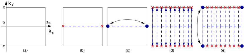
Figure 2: (a) BZ in $k$-space. (b) States are parallel transported along $k_{y}=0$, but are not periodic. (c) Periodicity is restored at $k_{y}=0$. (d) Parallel transport of states at all $k_{x}$ from $k_{y}=0$ to $k_{y}=\pm\pi$. (d) Periodicity is restored at $k_{x}=0$, and, hence, $k_{x}=2\pi$, but not at other $k_{x}$.

Parallel transport along $k_{y}$ at each $k_{x}$.

Next, at each mesh point $k_{x}$, we carry out two independent parallel-transport procedures, one from $(k_{x},0)$ to $(k_{x},\pi)$ along $+\hat{y}$ and another from $(k_{x},0)$ to $(k_{x},-\pi)$ along $-\hat{y}$. At each new $k_{y}$ point, the states are rotated by a unitary matrix so that the matrix of overlaps with the previous pair is as close to unity as possible. Starting this procedure from the line $k_{y}=0$ guarantees that the states on this line remain unchanged, preserving the smoothness obtained previously. Moreover, the entire parallel-transport procedure is identical at $k_{x}=0$ and $k_{x}=2\pi$, ensuring that the states selected in this way are continuous across the entire seam where $k_{x}=0$ has been glued to $k_{x}=2\pi$. Thus, we end up with two states defined everywhere on the mesh of $k$ points in such a way that they are smooth inside the BZ and periodic in $k_{x}$, or equivalently, smooth everywhere on the cylinder of Fig. 1(b). This step is illustrated in Fig. 2(d). The above procedure relates the states at $(k_{x},-\pi)$ to those at $(k_{x},\pi)$ by a unitary matrix

$$V_{mn}(k_{x})=\langle u_{m(k_{x},k_{y}=-\pi)}|\,{e^{2\pi iy}}\,|u_{n(k_{x},k_{y}=\pi)}\rangle,$$ (13)

which plays a role similar to $\Lambda$ of Eq. (37). This matrix encodes the information about the gauge discontinuity that occurs on the boundary of the cylindrical BZ. Its off-diagonal elements contain information about entanglement of the two states, while the diagonal ones carry information about phase discontinuity of the states.

Restoring periodicity in $k_{y}$ at $k_{x}=0$.

The fact that the two states at ${{\bf k}}=0$ form a Kramers pair guarantees that the matrix $V(k_{x})$ is diagonal at $k_{x}=0$ with two degenerate eigenvalues $\lambda(k_{x}=0)=e^{i\varphi_{0}}$. (Incidentally, the same is true at $k_{x}=\pi$; we use this fact later.) Now we want to restore the smoothness across $k_{y}=\pm\pi$ at $k_{x}=0$, but in such a way as to preserve the smoothness inside the cylindrical BZ. We do this by multiplying all states by a phase factor that depends smoothly on $k_{y}$ only:

$$|u_{n(k_{x},k_{y})}^{\rm new}\rangle=e^{-ik_{y}\varphi_{0}/2\pi}|u_{n(k_{x},k_{y})}\rangle$$ (14)

After this transformation, the $V(k_{x})$ matrix is the identity at $k_{x}$=0. Thus, the gauge discontinuity, which has already been segregated to the edges at $k_{y}=\pm\pi$, has now been further excluded from the point lying at $k_{x}$=0 (or $2\pi)$ on the edge. Fig. 2(e) illustrates this, where red crosses on the edges represent the gauge discontinuity and the black dots indicate continuity.

Note that the entire procedure up to this point preserves the TR symmetry, so that the states obtained so far on the BZ respect the constraints

$$\theta|u_{1{\bf k}}\rangle = |u_{2-{\bf k}}\rangle,$$

$$\theta|u_{2{\bf k}}\rangle = -|u_{1-{\bf k}}\rangle.$$ (15)

This in turn implies that

$$V(-k_{x})=\sigma_{y}\,[V(k_{x})]^{T}\,\sigma_{y}$$ (16)

so that ${\rm det}[V(-k_{x})]={\rm det}[V(k_{x})]$.

Removing the U(1) gauge discontinuity.

Obviously, $V(k_{x})\in\mathrm{U}(2)$, which can always be written as a $\mathrm{U}(1)$ phase times an $\mathrm{SU}(2)$ matrix. For our next step, we find it convenient to reduce $V(k_{x})$ to $\mathrm{SU}(2)$ form by multiplying the states $|u_{n{\bf k}}\rangle$ by a ${\bf k}$-dependent phase factor. To do so, we define

$$\gamma(k_{x})=\mathrm{Im}\log\det V(k_{x})$$ (17)

with the branch choice that $\gamma=0$ at $k_{x}$=0 and $\gamma(k_{x})$ is a continuous function of increasing $k_{x}$. This results in $\gamma=0$ again at $k_{x}=2\pi$ because the TR symmetry forces the total Chern number $C$ of the two bands to be zero. Indeed, $C$ is just given by the winding number of the $\mathrm{U}(1)\rightarrow\mathrm{U}(1)$ mapping from $k_{x}$ to $\gamma$. This follows from

$$2\pi C = \int_{0}^{2\pi}dk_{x}\,\left[\mathrm{Tr}\,{\cal A}_{k_{x}}^{(k_{y}=-\pi)}-\mathrm{Tr}\,{\cal A}_{k_{x}}^{(k_{y}=\pi)}\right]$$ (18)

$$= \int_{0}^{2\pi}dk_{x}\,\mathrm{Im}\mathrm{Tr}\left[V^{\dagger}\partial_{k_{x}}V\right]$$

$$= \int_{0}^{2\pi}dk_{x}\,\partial_{k_{x}}\gamma(k_{x})$$

$$= \gamma(k_{x})\Big{|}^{2\pi}_{0}$$

after some algebra.

Thus, our next step is simply to shift the phases of all states according to

$$|u_{n(k_{x},k_{y})}^{\rm new}\rangle=e^{-i\gamma(k_{x})k_{y}/4\pi}|u_{n(k_{x},k_{y})}\rangle.$$ (19)

This conserves all of the previous properties (smooth gauge inside the cylindrical BZ and on all boundaries except at $k_{y}=\pm\pi$). Moreover, $V(k_{x}=0)$ is still the identity, but now in addition, $\mathrm{det}\,V(k_{x})$ is real and positive at all $k_{x}$. That is, $V(k_{x})$ has been reduced to $\mathrm{SU}(2)$ form. We also note that Eqs. (15) and (16) continue to hold. However, $V(k_{x})$ remains off-diagonal at general $k_{x}$, thus signaling that the decomposition of the occupied subspace into the direct sum of the two TR-symmetric subspaces is not yet complete.

As noted earlier, the fact that our procedure starts from Kramers-degenerate pairs at $(k_{x},k_{y})=(0,0)$ and $(\pi,0)$ and respects TR symmetry at all stages enforces that $V(k_{x})$ must be a constant times the identity at $k_{x}=0$ and $k_{x}=\pi$. Since $V\in\mathrm{SU}(2)$ as well, $V$ must be $I$ or $-I$ at these two $k_{x}$ values. Previous gauge-fixing choices insure that $V(0)=I$, but is $V(\pi)=I$ or $-I$? It can be shown that these choices correspond to the case of the $Z_{2}$ index being even or odd, respectively. Indeed, according to homotopy theory, the mapping $\mathrm{U(1)}\rightarrow\mathrm{SU(2)}$ is characterized by a $Z_{2}$ index; this is precisely the case here. In fact, the procedure up to this point can be used as an alternative to the method we presented earlier in Ref. Soluyanov-PRB11-b, to compute the $Z_{2}$ invariant. From the numerical perspective, however, such a method does not have any significant advantages compared to the previously suggested one, apart from its straightforward geometric interpretation. In fact, for large systems it might not be very convenient to carry out all the transformations of the wavefunctions described above.

In what follows, we assume that the $Z_{2}$ index is odd.

III.2 Disentangling the two bands

In order to proceed, we want to make $V(k_{x})$ diagonal at each $k_{x}$. When this is accomplished we will have two disentangled bands 1 and 2, although each will still have its own phase discontinuity along the boundaries at $k_{y}=\pm\pi$. We take a first step in this direction by taking advantage of the freedom that we had when choosing the initial representatives of the occupied subspace at ${\bf k}=(0,0)$. These two states may be changed by a unitary transformation ${\cal U}$, which we take to belong to $\mathrm{SU(2)}$ so that the TR symmetry is fully preserved. So, we first look for the global $\mathrm{SU(2)}$ rotation that will minimize the sum of all the off-diagonal terms of the $V$ matrices at all $k_{x}$. Once this is done, a further adjustment can be made so as to make $V(k_{x})$ exactly diagonal at each $k_{x}$ without losing smoothness on the cylinder. We now explain the procedure in detail.

III.2.1 Steepest-descent minimization of ${\cal V}_{\rm OD}$

Let us introduce a functional

$${\cal V}_{\rm OD}=\frac{1}{N_{x}}\sum_{k_{x}}\sum_{m\neq n}|V_{mn}(k_{x})|^{2}$$ (20)

that is a measure of the degree to which $V(k_{x})$ fails to be diagonal along the discontinuity at $k_{y}=\pm\pi$. The sum on $k_{x}$ runs over a uniform grid of $N_{x}$ mesh points. We want to use the freedom of choosing the initial pair of states at ${{\bf k}}=(0,0)$ to minimize this functional by rotating the states at all $k$-points by the same unitary matrix ${\cal U}_{0}$. To do so, we consider the gradient of ${\cal V}_{\rm OD}$ with respect to an infinitesimal $k$-independent unitary transformation

$$U_{mn}=\delta_{mn}+dW_{mn},$$ (21)

where $dW=-dW^{\dagger}$ for $U$ to be unitary. A transformation of this form rotates the states according to

$$|\tilde{u}_{n{\bf k}}\rangle=|u_{n{\bf k}}\rangle+\sum_{m}dW_{mn}|u_{m{\bf k}}\rangle.$$ (22)

To first order in $dW$ the change in $V(k_{x})$ is

$$dV_{mn}=\left[V,dW\right]_{mn}\,.$$ (23)

To compute the gradient

$$G_{mn}=\left(\frac{d{\cal V}_{\rm OD}}{dW}\right)_{mn}=\;\frac{d{\cal V}_{\rm OD}}{dW_{nm}}$$ (24)

we note that Eq. (20) can be rewritten in the form

$${\cal V}_{\rm OD}={\cal N}-\frac{1}{N_{x}}\sum_{k_{x}}\sum_{n}^{\cal N}|V_{nn}(k_{x})|^{2}.$$ (25)

Then, using Eq. (23), one can write

$$d{\cal V}_{\rm OD} = -\frac{2}{N_{x}}\mathrm{Re}\sum_{k_{x}}\sum_{nm}V_{nn}^{*}(V_{nm}dW_{mn}-dW_{nm}V_{mn})$$ (26)

$$= -\frac{2}{N_{x}}\sum_{k_{x}}\mathrm{Re\,Tr}\left[R(k_{x})\,dW\right]$$

(the $k_{x}$ dependence of $V$ is suppressed for brevity) and

$$R_{mn}(k_{x})=V_{nm}[V_{nn}^{*}-V_{mm}^{*}].$$ (27)

The second line of Eq. (26) is obtained by interchanging the dummy $nm$ indices in the second term of the first line. It then follows that

$$G=\frac{1}{N_{x}}\sum_{k_{x}}\left[R(k_{x})-R^{\dagger}(k_{x})\right].$$ (28)

We emphasize that the gradient $G$ is independent of $k_{x}$ since it generates a global unitary rotation to be applied simultaneously to all states. Also, $G$ is not only antihermitian but also traceless, so that it generates a $\mathrm{SU(2)}$ unitary rotation. We now follow an iterative steepest-descent procedure, choosing a small positive damping constant $\beta$ and letting $dW=-\beta G^{\dagger}$ (i.e, $dW=\beta G$) so that $d{\cal V}_{\rm OD}=\mathrm{Tr}[G\,dW]=-\beta||G||^{2}$ to first order in $\beta$. We use this to update the states according to

$$|u_{n}^{(j+1)}\rangle=\sum_{m}\left[e^{\Delta W^{(j+1)}}\right]_{mn}|u_{n}^{(j)}\rangle$$ (29)

and the $V$ matrices according to

$$V^{(j+1)}=\left[e^{\Delta W^{(j+1)}}\right]^{\dagger}V^{(j)}e^{\Delta W^{(j+1)}}$$ (30)

where the upper index refers to the iteration step. The iteration stops when ${\cal V}_{\rm OD}^{(j)}-{\cal V}_{\rm OD}^{(j+1)}$ stays consistently below some pre-chosen tolerance $\varepsilon$.

To give a flavor of how steepest descent works we give the values obtained for the Kane-Mele model in the QSH regime ($\lambda_{v}/t=1$, $\lambda_{SO}/t=0.6$, $\lambda_{R}/t=0.5$) with a $120\times 120$ $k$-mesh, $\varepsilon=10^{-6}$ and $\beta=0.25$. Initially ${\cal V}_{\rm OD}=0.0226$, while after minimization ${\cal V}_{\rm OD}=0.0021$, so it becomes approximately ten times smaller. The crucial thing is that this final value of ${\cal V}_{\rm OD}$ suggests that the average off-diagonal element of $V$ has is of order $\times 10^{-2}$, meaning that the $V$ matrix is almost diagonal.

Note that at this stage the two subspaces are still not completely disentangled into two well-defined Chern subspaces. However, the gauge is very close to what we need. For example, the winding of $V(k_{x})$ already has the necessary features: if one plots $V_{11}$ in the complex plane as a function of $k_{x}$, one will see that it winds once around the origin in the counterclockwise direction as $k_{x}$ goes from $0$ to $2\pi$, as illustrated in Fig. 3.

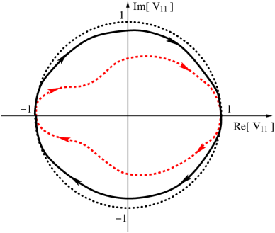
Figure 3: Trajectory of $V_{11}$ in the complex plane as $k_{x}$ runs across the BZ, before (red dashed line) and after (solid black line) the global ${\cal U}_{0}$ rotation that minimizes ${\cal V}_{\rm OD}$ for a ${\mathbb{Z}_{2}}$-odd insulator. In neither case is the graph exactly a unit circle (dotted line), but $V_{11}(0)=1$ and $V_{11}(\pi)=-1$.

Since $V$ are not diagonal yet the trace is not the unit circle, although it is close. $V_{22}$ winds in the opposite direction.

III.2.2 Diagonalization and final decomposition

Now we are in a position to make the final step in decomposition procedure. As a result of the steps above, the off-diagonal elements of the $V(k_{x})$ matrices should be small compared to the diagonal ones, so that the matrices are almost diagonal. This means that $V(k_{x})$ can be diagonalized by a unitary transformation ${\cal U}(k_{x})$ that is only slightly different from the unit matrix. Since diagonalization of $V(k_{x})$ does not fix the phases of the eigenvectors, and we need the phases to vary smoothly, we need an extra step to fix these phases. We do this by enforcing that the dominant component of each eigenvector of $V(k_{x})$ is real and positive. We then apply ${\cal U}(k_{x})$ to rotate the states at all $k_{y}$ for each given $k_{x}$ (except at $k_{x}=0$ or $\pi$, where $V$ was already diagonal).

As a result of this step the occupied subspace has been disentangled into a direct sum of two subspaces corresponding to states $n=1$ and 2. Moreover, they should form Kramers pairs and satisfy the constraint (15). Each subspace has a gauge that is smooth on the cylinder but not on the torus, since there is still a phase mismatch, corresponding to $V_{nn}(k_{x})$, across the boundary at $k_{y}=\pm\pi$. For the $Z_{2}$-odd case this phase discontinuity can never be completely removed, since the subspaces have Chern numbers of $\pm 1$.

To check the procedure, we apply it to the Kane-Mele model and compute the individual Chern numbers of the two disentangled bands. The computation is done for each band separately using the Abelian definition of Berry curvature, Eq. (3). The result is $C_{1}=-1$ and $C_{2}=+1$. The fact that the two states have well-defined Chern numbers is a signature of disentanglement, so that the individual Chern numbers of Eq. (12) have integer values ($c_{1}=-c_{2}=-1$). The TR constraint of Eq. (15) is indeed respected at each $k$-point. Thus we conclude that we have succeeded in finding a decomposition of the occupied subspace into a direct sum of two Chern subspaces that are mapped onto each other by the TR symmetry. Once again, we see that the TR-symmetric gauge for topological insulators is discontinuous on the BZ torus.

III.3 Establishing a cylindrical gauge

In Sec. II.1 we introduced a special “cylindrical gauge” for which the states satisfy Eq. (5). The defining characteristic of this special gauge is that the phase discontinuity at the cylinder boundary evolves at a constant rate as a function of $k_{x}$. As we shall see in Sec. IV, it is useful to have such a “standard gauge” enforced on the states when using them in some subsequent operations. Here we show how to extend our procedure so as to conform to the requirements of the cylindrical gauge.

As was mentioned above, the diagonal elements of $V(k_{x})$ wind around zero in the complex plane in opposite directions, changing by $2\pi$ when $k_{x}$ goes from $0$ to $2\pi$. Since we have carried out the diagonalization of the $V$ matrices, we know that the $V_{jj}$ elements follow a unit circle in the complex plane of the form $e^{i\rho_{j}(k_{x})}$. However, the speed of this rotation given by $v_{j}(k_{x})=d\rho_{j}/dk_{x}$ (where $\rho_{j}$ remains on the same branch of the logarithm) is not constant, in contrast to the requirement of the cylindrical gauge.

To change the speed of winding of $V(k_{x})$ we apply the gauge transformation

$$W(k_{x},k_{y})=\left[V_{\rm targ}(k_{x})V^{\dagger}(k_{x})\right]^{k_{y}/2\pi}$$ (31)

to the the occupied states at each $(k_{x},k_{y})$. Here

$$V_{\rm targ}(k_{x})=\begin{pmatrix}e^{ik_{x}c_{1}}&0\\ 0&e^{ik_{x}c_{2}}\end{pmatrix}.$$

gives the target shape of $v$ that corresponds to the cylindrical gauge. Note that the choice of sign should be correlated with the individual Chern number of the band it is applied to. Such a gauge transformation is obviously continuous on the cylinder and does not change the topology of the individual bands. It also preserves the TR symmetry of the states and the relation of Eq. (15) is still satisfied.

We note that if the above decomposition is applied to a normal insulator (say, the Kane-Mele model in the normal-insulator regime), then $c_{1}=c_{2}=0$ and a smooth gauge is obtained at this step.

III.4 Relation to spin Chern numbers

Finally, we would like to compare our approach to disentangling ${\mathbb{Z}_{2}}$ bands into Chern bands to some other approaches suggested previously. In the work of Ref. Sheng-PRL06, the authors suggested to associate a Chern number with each possible spin projection value. This is especially convenient when $\hat{s}_{z}$ is conserved; then it is natural to assign individual Chern numbers to each of the bands identified by a particular value of $s_{z}$. Such Chern numbers were called “spin Chern numbers.” For example, in the case of the Kane-Mele model with no Rashba coupling (i.e., $\lambda_{R}=0$), $\hat{s}_{z}$ is conserved and the Hamiltonian becomes block-diagonal with respect to the spin projection, allowing for well-defined spin Chern numbers. When the Rashba interaction is turned on the mirror symmetry of the model is broken and $\hat{s}_{z}$ is no longer conserved, thus making the original concept of a spin Chern number obscure.

This issue was clarified further by Prodan,Prodan-PRB09 who showed that even with the spin-mixing Rashba term it is possible to define spin Chern numbers by diagonalizing $\hat{s}_{z}$ in the occupied space of ${\mathbb{Z}_{2}}$ insulator at each ${\bf k}$. In other words, one diagonalizes the operator $\hat{P}_{{\bf k}}\hat{s}_{z}\hat{P}_{{\bf k}}$, where $\hat{P}_{{\bf k}}$ is the projector onto the occupied states at ${\bf k}$. Then, if the eigenvalues turn out to be separated by a spectral gap from one another at each value of ${\bf k}$, one can identify these “bands” as the desired manifolds, and carry out a unitary rotation of the original bands into these states to disentangle them. The spin Chern numbers thus defined for these bands are well defined and, in fact, correspond to the individual Chern numbers of our work. However, when the spectral gap between any two eigenvalues of the projected spin operator closes, such a decomposition becomes impossible. One could still consider some other projection operators based on mirror or other symmetries, as in Ref. Teo-PRB08, , and use these eigenvalues in a similar way to disentangle the occupied states. However, such a method always relies on some symmetry of a particular model, and is thus not universal. The method suggested in the present work, in contrast, does not depend on any symmetries of the underlying system. Thus, we conclude that individual Chern numbers proposed in the present work are robust and arise solely from the topology of the occupied subspace of the system.

Finally, it was discussed elsewhere that the spin Chern numbers do not contain any more information than the ${\mathbb{Z}_{2}}$ invariant, because their sign can be changed without closing the insulating gap.Fu-PRB06 ; Fukui-PRB07 ; Prodan-PRB09 This is the case for individual Chern numbers as well, since obviously, one can simply change the labeling of the states by a simple unitary transformation that interchanges $|u_{1{\bf k}}\rangle$ with $|u_{2{\bf k}}\rangle$. Therefore, individual Chern numbers are merely an alternative way of describing the occupied subspace of a ${\mathbb{Z}_{2}}$ insulator in terms of disentangled bands, and do not contain any more information about the topological state of the whole system than a ${\mathbb{Z}_{2}}$ invariant alone.

IV Rotation into a smooth gauge

We now discuss the final step in our construction of a smooth gauge for a QSH insulator starting from the two Chern bands obtained at the previous steps. The task of unwinding the topological twists of these bands requires a unitary transformation that is also topologically nontrivial in the following sense. Obviously, a transformation that is smooth on the BZ torus, being periodic in the $k_{y}$ direction, cannot make a cylindrical gauge smooth. One needs instead a unitary transformation ${\cal G}({\bf k})\in{\mathrm{U}(2)}$ that has a discontinuity on the torus that exactly cancels out the discontinuities of the cylindrical-gauge states. Of course, since the total Chern number of the whole occupied space is a topological invariant,Avron-PRL83 the transformation will preserve the condition that the total Chern number is zero. In particular, the rotation we are looking for makes $c_{1}=c_{2}=0$.

A unitary transformation that solves the problem of unwinding the two QSH bands with Chern numbers $\pm 1$ is given naturally by the solution of the Haldane modelHaldane-PRL88 of a Chern insulator (CI), or for that matter, of any two-band model of a CI. Indeed, the unitary transformation ${\cal G}({\bf k})$ that diagonalizes the Hamiltonian in that case is one that rotates the two topologically trivial tight-binding basis states $(1,0)^{T}$ and $(0,1)^{T}$ into the eigenstates of the model. Obviously, ${\cal G}^{-1}({\bf k})={\cal G}^{\dagger}({\bf k})$ rotates the topologically nontrivial states back into the trivial ones, and thus can be used to unwind our QSH states. In order for this procedure to produce a smooth gauge, the Hamiltonian eigenstates of the CI model also have to be smoothly defined on the cylinder and obey the same cylindrical gauge of Eqs. (4-5). Assuming this has been done, the application of the resulting ${\cal G}^{\dagger}({\bf k})$ to the QSH states defined by our procedure will finally result in a gauge that is smooth everywhere on the torus and that generates new bands with $c_{1}=c_{2}=0$, as desired.

The numerical implementation of this procedure is done most conveniently by solving the CI model on the same 2D ${\bf k}$-space mesh as was used to solve for the QSH states. If the latter have been computed in the context of first-principles calculations or of some complex tight-binding model, then some known CI model such as the Haldane model can be used to provide the needed ${\cal G}({\bf k})$. However, when working with a minimal $4\times 4$ tight-binding model for a QSH system, it may be more convenient to use a $2\times 2$ spin-up (or spin-down) block of the original $4\times 4$ QSH model itself. After all, this already lives on the needed ${\bf k}$-mesh and generates bands with Chern numbers of $\pm 1$. For example, for an application to the Kane-Mele model in the QSH regime ($\lambda_{v}/t=1$, $\lambda_{SO}/t=0.6$, $\lambda_{R}/t=0.5$), we used the spin-up block of the original Hamiltonian and obtained two states $|{u}_{i{\bf k}}^{\prime}\rangle$ with Chern numbers ${c}_{1}^{\prime}=-1$ and ${c}_{2}^{\prime}=1$, where the hat is used to distinguish the CI quantities from the QSH ones.

As mentioned earlier, it is also necessary to bring the CI bands $|{u}^{\prime}_{i{\bf k}}\rangle$ into the cylindrical gauge in order to ensure that the resulting ${\cal G}^{\dagger}({\bf k})$ exactly cancels the discontinuity of the QSH bands at the edge of the cylinder. For this purpose, a parallel-transport procedure is carried out across the BZ in close analogy to what was described in Sec. III.1, but now it is done in a single-band $\mathrm{U(1)}$ context applied to each of the CI states in turn. It is useful to refer again to Fig. 2. First, a parallel transport of $|{u}^{\prime}_{1{\bf k}}\rangle$ is carried out along the $k_{x}$ axis (with an arbitrary choice of phase at ${\bf k}=0$), and a graded phase twist is applied to match phases at $k_{x}=0$ and $2\pi$ as in Figs. 2(b-c). Then parallel transport is performed along the vertical directions as in Fig. 2(d), and a ($k_{x}$-independent) phase change that is graded along $k_{y}$ is applied to restore continuity at the corner points of Fig. 2(e). This defines a phase discontinuity ${V}^{\prime}_{11}(k_{x})=\langle{u}^{\prime}_{1}(k_{x},-\pi)|{u}^{\prime}_{1}(k_{x},\pi)\rangle$ whose phase-winding rate $d\,\ln(V_{11})/dk_{x}$ is initially nonuniform, but is made uniform by the same trick as for the QSH states. The procedure is repeated for the second CI band.

The above procedure results in Chern bands obeying the cylindrical gauge as required. We can now simply form the desired unitary matrix ${\cal G}({\bf k})$ as the $2\times 2$ matrix whose first and second columns are filled with the column vectors $|{u}^{\prime}_{1}({\bf k})\rangle$ and $|{u}^{\prime}_{2}({\bf k})\rangle$ respectively. We emphasize again that this matrix is not topologically trivial; its coefficients are continuous on the cylinder, but not continuous across $k_{y}=\pm\pi$, just like the CI that has produced it. Applying ${\cal G}^{\dagger}({\bf k})$ to the QSH bands constructed in Sec.III,

$$|\tilde{u}_{n{\bf k}}\rangle=\sum_{m}{\cal G}^{\dagger}_{mn}({\bf k})|u_{m{\bf k}}\rangle\,,$$ (32)

we finally end up with two bands that have $c_{1}=c_{2}=0$ and that span the Hilbert space defined by the original occupied bands of the QSH model. Thus, we have constructed a smooth and periodic gauge for the target ${\mathbb{Z}_{2}}$ insulator.

It should be stressed that rotation into a smooth gauge as described above breaks TR symmetry, since ${\cal G}({\bf k})$ results from a TR-broken CI model. Thus, the two smooth subspaces are not mapped onto each other by the TR operator, so that $\langle\tilde{u}_{1,{\bf k}}|\theta|\tilde{u}_{2,-{\bf k}}\rangle\neq 0$ except at TR-invariant momenta ${\bf k}=-{\bf k}+{\bf G}$. Similarly, if Wannier functions are constructed from the Bloch spaces defined in this way, they will not form Kramers pairs.Soluyanov-PRB11-a Finally, we note that although the gauge is now smooth and periodic, it can be smoothed further by using this gauge as a starting point for a Wannier-function maximal-localization procedure.Marzari-PRB97

In summary, we have demonstrated a general method for constructing a smooth gauge for a ${\mathbb{Z}_{2}}$ topological insulator. At this final stage we start with a gauge that still respects TR symmetry, but then we carry out a unitary mixing operation that violates this symmetry in order to avoid the topological obstruction. Application to the Kane-Mele model allows us to compute the ${\mathbb{Z}_{2}}$ invariant with the smooth-gauge formula of Fu and KaneFu-PRB06 as discussed in Appendix C.

V Conclusions

In this paper we have developed a general method for decomposing the occupied space of a ${\mathbb{Z}_{2}}$ insulator into a direct sum of two TR-symmetric Chern subspaces with nontrivial individual Chern numbers. We then described a general procedure for breaking the TR symmetry between the two bands and rotating them into subspaces that are smooth everywhere on the torus. Our methods are general in the sense that they do not make use of any special symmetries or assumptions about gaps in the spectrum of spin operators. This establishes the construction of a smooth gauge for 2D topological insulators.

Appendix A Parallel transport

Let us discuss how to construct a parallel-transport gauge starting from a set of randomly chosen eigenstates of the Hamiltonian on a ${\bf k}$-mesh. In what follows we distinguish single-band and multiband parallel transport procedures. The general idea in both cases is to carry the Bloch states along a certain path in the BZ in such a way that they remain as parallel as possible to the previous states at all points. If the path is closed, the states might return to the initial point with some phase differences relative to the initial states, thus violating singlevaluedness. However, singlevaluedness of the wavefunction can be restored by spreading the extra phase uniformly along the path, as explained in more detail below. For simplicity, we consider parallel transport along one direction in the BZ, say $k_{x}$. In this case, a closed loop is obtained when the state is transported by a reciprocal lattice vector ${\bf G}_{x}$. The generalization to an arbitrary direction should be obvious.

Consider a single isolated band $|u_{n{\bf k}}\rangle$. To carry the state to $k+\Delta k$ via parallel transport, the phase of the Bloch state at this new point should be chosen in such a way that the overlap $\langle u_{n{\bf k}}|u_{n,{\bf k}+\Delta k_{x}}\rangle$ is real and positive, so that the change in the state is orthogonal to the state itself. It is straightforward to implement this numerically. Consider a discrete uniform mesh of $k$-points $\{{\bf k}_{j}\},j\in[1,N+1]$, where ${\bf k}_{j+1}={\bf k}_{j}+\Delta k_{x}$ and ${\bf k}_{N+1}={\bf k}_{1}+{\bf G}_{x}$. The states $|\tilde{u}_{{\bf k}_{j}}\rangle$ at these points are obtained by a numerical diagonalization procedure and thus have random phases. At the initial point $j$=1 we set $|u^{\prime}_{{\bf k}_{1}}\rangle=|\tilde{u}_{{\bf k}_{1}}\rangle$. Then at each subsequent ${\bf k}_{j+1}$ we let $\beta_{j+1}={\rm Im}\,\ln\,\langle\tilde{u}_{{\bf k}_{j+1}}^{\phantom{,}}|\,u^{\prime}_{{\bf k}_{j}}\rangle$ and then apply the ${\cal U}(1)$ phase rotation

$$|u^{\prime}_{{\bf k}_{j+1}}\rangle=e^{i\beta_{j+1}}|\tilde{u}_{{\bf k}_{j+1}}\rangle\,,$$ (33)

which makes $\langle u^{\prime}_{{\bf k}_{j}}|u^{\prime}_{{\bf k}_{j+1}}\rangle$ real and positive. Once this is done at each ${\bf k}$-point, the state at ${\bf k}_{1}$ differs from that at ${\bf k}_{N+1}$ by a phase factor $e^{i\phi}$, where $\phi$ is chosen on a particular branch, say $\phi\in(-\pi,\pi]$. $\phi$ is the Berry phase associated with the traversed path. Unless $\phi=0$, periodicity in $k_{x}$ is lost. To restore it, the extra phase should be spread uniformly along the string of ${\bf k}$-points, i.e.,

$$|u_{{\bf k}_{j}}\rangle=e^{-i\phi{\bf k}_{j}/2\pi}|u^{\prime}_{{\bf k}_{j}}\rangle=e^{-i(j-1)\phi/N}|u^{\prime}_{{\bf k}_{j}}\rangle,$$ (34)

where in the last equality the uniformity of the $k$-mesh was used.

In the multiband case one deals with the non-Abelian generalization of the Abelian Berry phase.Wilczek-PRL84 ; Mead-RMP92 We now consider an isolated set of ${\cal N}$ bands and describe parallel transport in the $k_{x}$-direction in the non-Abelian case.Marzari-PRB97 ; Resta-JPC00 The parallel transport gauge is constructed by requiring that the overlap matrix

$$\tilde{M}_{mn}^{({\bf k}_{j},{\bf k}_{j+1})}=\langle\tilde{u}_{m{{\bf k}_{j}}}|\tilde{u}_{n{\bf k}_{j+1}}\rangle$$ (35)

must be Hermitian, with all positive eigenvalues, at each step. This is uniquely accomplished by means of the singular value decomposition in which an ${\cal N}\times{\cal N}$ matrix $M$ is written in the form $M=V\Sigma W^{\dagger}$, where $V$ and $W$ are unitary and $\Sigma$ is positive real diagonal. If the states at ${\bf k}_{j+1}$ are rotated by ${\cal U}=WV^{\dagger}$, i.e.,

$$|{u}^{\prime}_{n{\bf k}_{j+1}}\rangle=\sum_{m}^{\cal N}{\cal U}_{mn}({\bf k}_{j+1})|\tilde{u}_{m{\bf k}_{j+1}}\rangle,$$ (36)

the new overlap matrix ${M}_{mn}^{\prime\,{({\bf k}_{j},{\bf k}_{j+1})}}$ will be of the form $V\Sigma V^{\dagger}$, which is Hermitian with positive eigenvalues as desired. Repeating this procedure up to $j=N$, one obtains that the new states $|u^{\prime}_{n{\bf k}_{N+1}}\rangle$ are related to the states $|u^{\prime}_{n{\bf k}_{1}}\rangle$ by a unitary transformation $\Lambda$ according to

$$|u^{\prime}_{n{{\bf k}_{1}}}\rangle=e^{2\pi ix}\sum_{m}^{\cal N}\Lambda_{mn}|u^{\prime}_{m{{\bf k}_{N+1}}}\rangle.$$ (37)

The eigenvalues of this matrix are of the form $\lambda_{n}=e^{-i\phi_{n}}$, where the phases $\phi_{n}={\rm Im\,ln}\,\lambda_{n}$ (again chosen according to some definite branch cut) are the analogs of the Abelian Berry phases.

To restore periodicity we follow the same trick as in the single-band case, but generalized to the matrix form. To do this one finds the unitary matrix $R$ that diagonalizes $\Lambda$, and then rotates all states at all ${\bf k}_{j}$ by this same unitary $R$, so that the new states correspond to a diagonal $\Lambda$ with its eigenvalues $\lambda_{n}=e^{i\phi_{n}}$ on the diagonal. Now it is straightforward to obtain periodicity by applying the graded phase twists

$$|{u}_{n{\bf k}_{j}}\rangle=e^{-i(j-1)\phi_{j}/N}|u^{\prime}_{n{\bf k}_{j}}\rangle.$$ (38)

This results in a gauge that is smooth along $k_{x}$ and ${\bf G}_{x}$-periodic.

Appendix B Kane-Mele model

Here we briefly summarize the Kane-Mele model Kane-PRL05-b of a quantum spin Hall system. This model is represented by a tight-binding (TB) Hamiltonian on a honeycomb lattice with dimensionless lattice vectors $a_{1,2}=(\sqrt{3}\hat{\bf y}\pm\hat{\bf x})/2$. The Hamiltonian is

$$H=\lambda_{v}\sum_{i}\xi_{i}c_{i}^{\dagger}c_{i}+\sum_{<ij>}c_{i}^{\dagger}\left(t+i\lambda_{R}[{\bf s}\times{\hat{\bf d}}_{ij}]_{z}\right)c_{j}$$

$$+i\lambda_{SO}\sum_{\ll ij\gg}\nu_{ij}c_{i}^{\dagger}s^{z}c_{j},$$ (39)

where the three terms represent on-site, first-, and second-neighbor interactions respectively. Here $\xi_{i}=\pm 1$ represents a staggered on-site interaction (breaking the inversion symmetry of the original honeycomb lattice), and $\lambda_{SO}$ and $\lambda_{R}$ represent the effects of spin-orbit interaction (the latter breaks $S_{z}$ conservation and violates mirror symmetry in the $xy$-plane). Also, $\hat{\bf d}_{ij}$ is a unit vector directed from site $i$ to site $j$, while $\nu_{ij}=(2/\sqrt{3})[\hat{\bf d}_{1}\times\hat{\bf d}_{2}]=\pm 1$, where $\hat{\bf d}_{1}$ and $\hat{\bf d}_{2}$ represent the directions of the two bonds along which the electron hops in going from site $i$ to site $j$.

Using the TB convention $\chi_{j\sigma{\bf k}}({\bf r})=\sum_{{\bf R}}e^{i{\bf k}\cdot{\bf R}}\varphi_{s}({\bf r}-{\bf R}-{\bf t}_{j})$, where $\varphi$ are TB basis functions, $s$ stands for the spin index, and ${\bf t}_{j}$ is the vector from the origin to the $j$-th atom in the home unit cell, the Hamiltonian is written as

$$H({\bf k})=\sum_{\alpha=1}^{5}d_{\alpha}({\bf k})\Gamma^{\alpha}+\sum_{\alpha<\beta=1}^{5}d_{\alpha\beta}({\bf k})\Gamma^{\alpha\beta}.$$ (40)

Here the Dirac matrices are $\Gamma^{1,2,3,4,5}=(I\otimes\sigma^{x},I\otimes\sigma^{z},s^{x}\otimes\sigma^{y},s^{y}\otimes\sigma^{y},s^{z}\otimes\sigma^{y})$ with the Pauli matrices $\sigma^{k}$ and $s^{k}$ acting in sublattice and spin space respectively, and the commutators are $\Gamma^{\alpha\beta}=[\Gamma^{\alpha},\Gamma^{\beta}]/(2i)$. The original reciprocal-lattice coordinates ${\kappa_{1}}$ and $\kappa_{2}$ may be changed into $k_{x}\in[0,2\pi]$ and $k_{y}\in[-\pi,\pi]$ via $k_{x}=\kappa_{x}/2-\sqrt{3}\kappa_{y}/2$ and $k_{y}=\kappa_{x}/2+\sqrt{3}\kappa_{y}/2$. The resulting $d$ coefficients are given in Table 1.

$d_{1}$	$t(1+2\cos{\alpha}\cos{\beta})$	$d_{12}$	$-2t\cos{\alpha}\sin{\beta}$
$d_{2}$	$\lambda_{v}$	$d_{15}$	$2\lambda_{SO}(\sin{2\alpha}-2\sin{\alpha}\cos{\beta})$
$d_{3}$	$\lambda_{R}(1-\cos{\alpha}\cos{\beta})$	$d_{23}$	$-\lambda_{R}\cos{\alpha}\sin{\beta}$
$d_{4}$	$-\sqrt{3}\lambda_{R}\sin{\alpha}\sin{\beta}$	$d_{24}$	$\sqrt{3}\lambda_{R}\sin{\alpha}\cos{\beta}$

Table 1: Nonzero coefficients in Eq. (40). Here $\alpha=(k_{x}+k_{y})/2$ and $\beta=(k_{y}-k_{x})/2$ with $k_{x}=\kappa_{x}/2-\sqrt{3}\kappa_{y}/2$ and $k_{y}=\kappa_{x}/2+\sqrt{3}\kappa_{y}/2$. The lattice constant is assumed to be of unit length.

This model respects time-reversal symmetry and realizes the QSH regime, i.e., it represents a 2D ${\mathbb{Z}_{2}}$ topological insulator in some regions of its parameter space.Kane-PRL05-b For our illustrative tests we have used $\lambda_{v}/t=1$, $\lambda_{SO}/t=0.6$ and $\lambda_{R}/t=0.5$ for the topological phase, and have changed $\lambda_{v}/t$ to $5$ to access the normal phase.

Appendix C Time-reversal constraint and smooth gauge

In Ref. Fu-PRB06, Fu and Kane developed a theory of a ${\mathbb{Z}_{2}}$ periodic spin pump of a 1D insulating system. That work established a formula for computing the ${\mathbb{Z}_{2}}$ invariant given a smooth gauge. In this Appendix we review this result and discuss it from the perspective of the smooth gauge constructed in the present work.

The work of Ref. Fu-PRB06, focuses on the pumping process in 1D gapped periodic Hamiltonians subject to the conditions $H(t+T)=H(t)$ and $H(-t)=\theta H(t)\theta^{-1}$, where $t$ is the pumping parameter. Such a pump becomes TR-invariant at $t=0$ and $t=T/2$. The Hamiltonian of a 2D TR-symmetric insulator can easily be put in this context by treating $k_{x}$ as the wavevector $k$ of a 1D periodic system while treating $k_{y}$ as the pumping parameter $t$. Assuming at the TR-invariant values of $t$ a gauge of the form

$$\theta|u_{1k}\rangle = e^{i\chi_{k}}|u_{2-k}\rangle$$

$$\theta|u_{2k}\rangle = -e^{i\chi_{-k}}|u_{1-k}\rangle,$$ (41)

that is smooth in $k$, it was shown that one can compute the ${\mathbb{Z}_{2}}$ invariant associated with the pumping process from a knowledge of the occupied states at the TR-invariant points of the pumping cycle only. However, for this purpose the gauge must be smooth on the whole torus formed by $k$ and $t$.Fu-PRB06

Let us now look at how all this is reformulated in terms of the gauges introduced in the present paper for a 2D system. The Hamiltonian gauge of an ordinary TR-symmetric insulating system corresponds to $\chi_{k}=0$ in Eq. (41), and it is possible to define Bloch states in a smooth fashion on the whole torus subject to this condition. However, for a ${\mathbb{Z}_{2}}$ insulator such a constraint introduces a topological obstruction for a smooth gauge.Fu-PRB06 This can be understood in terms of the cylindrical gauge introduced in Sec. II. Taking into account that the TR-symmetric values of the pumping parameter now correspond to $k_{y}=0$ and $k_{y}=\pm\pi$, note that in the cylindrical gauge the TR operator maps the states at $(k_{x},k_{y}=0)$ to $(-k_{x},k_{y}=0)$ and the states at $(k_{x},k_{y}=\pm\pi)$ to $(-k_{x},k_{y}=\mp\pi)$ according to Eq. (15). If we now take into account the boundary conditions of Eq. (5) for the cylindrical gauge and use them to relate the states at $(k_{x},k_{y})$ to those at $(-k_{x},k_{y})$, one then arrives at a relation of the form of Eq. (41) with

$$\chi_{k}=0$$

at $k_{y}=0$ and

$$\chi_{k}=\pm k_{x}C$$

at $k_{y}=\pm\pi$. For an ordinary insulator $C=0$, and this obviously reduces to the standard case of $\chi_{k}=0$ both at $k_{y}=0$ and $k_{y}=\pm\pi$.

To derive an expression for the ${\mathbb{Z}_{2}}$ invariant a concept of partial polarization was introducedFu-PRB06 using the gauge of Eq. (41) via

$$P^{(S)}_{t}=\frac{1}{2\pi}\left[i\int_{0}^{\pi}\langle u_{S,t,k}|\partial_{k}|u_{S,t,k}\rangle dk+(\chi_{t,k=\pi}-\chi_{t,k=0})\right]$$ (42)

where the index $S=1,2$ differentiates between the two states of a Kramers pair. This expression is $\mathrm{U(2)}$ invariant modulo a lattice vector ($a=1$), provided that the transformation is globally smooth in 1D. The ${\mathbb{Z}_{2}}$ invariant was defined as

$$\nu=(P^{(1)}_{t=0}-P^{(2)}_{t=0})-(P^{(1)}_{t=T/2}-P^{(2)}_{t=T/2}),$$ (43)

when the gauge is also smooth in $t$ from $0$ to $T/2$. With the $\chi_{k}$ suggested by the cylindrical gauge, and taking into account that $C$ has opposite sign for $S=1$ and $S=2$, one has $P^{(1)}_{k_{y}=0}-P^{(2)}_{k_{y}=0}=0$ and $P^{(1)}_{k_{y}=\pm\pi}-P^{(2)}_{k_{y}=\pm\pi}=\pm C$, obviously giving the correct value of the topological invariant.

As shown above, the construction of a smooth gauge starting with the cylindrical gauge proceeds by means of a unitary rotation that unwinds the gauge discontinuity of the cylindrical gauge. The unitary matrix that realizes this transformation is smooth and periodic in $k_{x}$. Thus, when establishing a smooth gauge at the TR-invariant values of $k_{y}$ the gauge condition (41) on the 1D system is changed smoothly and, as discussed in Sec. IV, the smooth occupied subspaces are no longer mapped onto each other by $\theta$. However, the TR polarization does not change under such a transformation, and as was nicely shown in Ref. Fu-PRB06, , one can compute the ${\mathbb{Z}_{2}}$ index using the formula

$$(-1)^{\nu}=\prod_{i=1}^{4}\frac{\sqrt{\det[w({\bf k}^{*}_{i})]}}{\mathrm{Pf}[w({\bf k}^{*}_{i})]},$$ (44)

where ${\bf k}^{*}$ are TR-invariant momenta (i.e., ${\bf k}^{*}=-{\bf k}^{*}+{\bf G}$) and

$$w_{ij}({\bf k})=\langle u_{i-{\bf k}}|\theta|u_{j{\bf k}}\rangle.$$ (45)

Note, that $w(-{\bf k}^{*})=-w^{T}({\bf k}^{*})$, so that the Pfaffian in (44) is well defined.

The application of the smooth-gauge construction developed in the main text of this paper to the Kane-Mele model in the QSH regime indeed results in the odd value for $\nu$. The TR constraint takes the form $w_{12}({\bf k}^{*})=\pm 1$ and, as mentioned above, is satisfied only at the TR-invariant momenta, with $|w_{12}({\bf k})|<1$ at other values of ${\bf k}$. In particular, our parameter choice ($\lambda_{v}/t=1$, $\lambda_{SO}/t=0.6$, $\lambda_{R}/t=0.5$) results in $w_{12}(0,0)=1$ but $w_{12}(0,\pi)=w_{12}(\pi,0)=w_{12}(\pi,\pi)=-1$, thus signaling a band inversion at $\Gamma=(0,0)$.

References

- (1) M. V. Berry, Proc. R. Soc. Lon. A 392, 45 (1984)
- (2) Y. Aharonov and D. Bohm, Phys. Rev. 115, 485 (1959)
- (3) R. D. King-Smith and D. Vanderbilt, Phys. Rev. B 47, 1651 (1993)
- (4) R. Resta, Rev. Mod. Phys. 66, 899 (1994)
- (5) D. J. Thouless, M. Kohmoto, M. P. Nightingale, and M. den Nijs, Phys. Rev. Lett. 49, 405 (1982)
- (6) F. D. M. Haldane, Phys. Rev. Lett. 93, 206602 (2004)
- (7) M. Z. Hasan and C. L. Kane, Rev. Mod. Phys. 82, 3045 (2010)
- (8) X.-L. Qi and S.-C. Zhang, Rev. Mod. Phys. 83, 1057 (2011)
- (9) A. Kitaev, AIP Conf. Proc. 1134, 22 (2009)
- (10) A. P. Schnyder, S. Ryu, A. Furusaki, and A. W. W. Ludwig, Phys. Rev. B 78, 195125 (2008)
- (11) A. P. Schnyder, S. Ryu, A. Furusaki, and A. W. W. Ludwig, AIP Conf. Proc. 1134, 10 (2009)
- (12) F. D. M. Haldane, Phys. Rev. Lett. 61, 2015 (1988)
- (13) M. Kohmoto, Annals of Physics 160, 343 (1985)
- (14) M. Nakahara, Geometry, Topology and Physics (Taylor and Francis Group, 2003)
- (15) C. L. Kane and E. J. Mele, Phys. Rev. Lett. 95, 146802 (2005)
- (16) C. L. Kane and E. J. Mele, Phys. Rev. Lett. 95, 226801 (2005)
- (17) M. Konig, S. Wiedmann, C. Brune, A. Roth, H. Buhmann, L. W. Molenkamp, X.-L. Qi, and S.-C. Zhang, Science 318, 766 (2007)
- (18) B. A. Bernevig, T. L. Hughes, and S.-C. Zhang, Science 314, 1757 (2006)
- (19) B. A. Volkov and O. A. Pankratov, JETP Letters 42, 178 (1985)
- (20) D. J. Thouless, J. Phys. C 17, L325 (1984)
- (21) T. Thonhauser and D. Vanderbilt, Phys. Rev. B 74, 235111 (2006)
- (22) C. Brouder, G. Panati, M. Calandra, C. Mourougane, and N. Marzari, Phys. Rev. Lett. 98, 046402 (2007)
- (23) L. Fu and C. L. Kane, Phys. Rev. B 74, 195312 (2006)
- (24) R. Roy, Phys. Rev. B 79, 195321 (2009)
- (25) T. A. Loring and M. B. Hastings, EPL 92, 67004 (2010)
- (26) A. A. Soluyanov and D. Vanderbilt, Phys. Rev. B 83, 035108 (2011)
- (27) D. N. Sheng, Z. Y. Weng, L. Sheng, and F. D. M. Haldane, Phys. Rev. Lett. 97, 036808 (2006)
- (28) J. C. Y. Teo, L. Fu, and C. L. Kane, Phys. Rev. B 78, 045426 (2008)
- (29) E. Prodan, Phys. Rev. B 80, 125327 (2009)
- (30) N. Marzari and D. Vanderbilt, Phys. Rev. B 56, 12847 (1997)
- (31) D. Vanderbilt and R. D. King-Smith, Phys. Rev. B 48, 4442 (1993)
- (32) J. Zak, Phys. Rev. Lett. 62, 2747 (1989)
- (33) N. Marzari, A. A. Mostofi, J. R. Yates, I. Souza, and D. Vanderbilt arXiv:1112.5411
- (34) L. Fu and C. L. Kane, Phys. Rev. B 76, 045302 (2007)
- (35) T. Fukui and Y. Hatsugai, J. Phys. Soc. Jpn. 76, 053702 (2007)
- (36) A. A. Soluyanov and D. Vanderbilt, Phys. Rev. B 83, 235401 (2011)
- (37) R. Yu, X. L. Qi, A. Bernevig, Z. Fang, and X. Dai, Phys. Rev. B 84, 075119 (2011)
- (38) E. Prodan, Phys. Rev. B 83, 235115 (2011)
- (39) F. Wilczek and A. Zee, Phys. Rev. Lett. 52, 2111 (1984)
- (40) C. A. Mead, Rev. Mod. Phys. 64, 51 (1984)
- (41) J. E. Avron, R. Seiler, and B. Simon, Phys. Rev. Lett. 51, 51 (1983)
- (42) As an alternative, one could carry out a single-band parallel transport of the two resultant states along to smooth out the random phase variations at different introduced by the diagonalization procedure.
- (43) T. Fukui and Y. Hatsugai, Phys. Rev. B 75, 121403 (2007)
- (44) R. Resta, J. Phys. C 12, R107 (2000)