Abundance of attracting, repelling and elliptic periodic orbits in two-dimensional reversible maps.

Abstract

We study dynamics and bifurcations of two-dimensional reversible maps having non-transversal heteroclinic cycles containing symmetric saddle periodic points. We consider one-parameter families of reversible maps unfolding generally the initial heteroclinic tangency and prove that there are infinitely sequences (cascades) of bifurcations of birth of asymptotically stable and unstable as well as elliptic periodic orbits.

1 Introduction

Reversible systems have a very special status inside the realm of dynamical systems. Usually, they are positioned “between” dissipative and conservative systems. In the context of continuous dynamical systems, a reversibility means that the system is invariant under the change of time-direction, $t\mapsto-t$, and a transformation in the spatial variables. In the discrete context, reversibility of a map $f$ (a diffeomorphism) means that $f$ and $f^{-1}$ possess the same dynamics. Notice that the term “the same” can have rather different meaning. If $f$ and $f^{-1}$ are smoothly conjugate, i.e., $f\circ h=h\circ f^{-1}$ and $h$ is a just a diffeomorphism, then $f$ is called weekly reversible. However, much more interesting types of reversibility appear when $h$ possesses some structures. For example, if $h$ is an involution, i.e., $h^{2}=\mathrm{Id}$. In this case, the map $f$ is called strongly reversible. Since this last case is the most frequent one in the literature (probably, beginning with Birkhoff), nowadays strongly reversible maps are simply called reversible maps.

In contrast to conservative and dissipative systems, the study of homoclinic bifurcations in reversible systems is not so popular. Even for two-dimensional maps, only few results are known and most of them relate to “conservative and reversible” maps which form a certain codimension-$\infty$ subclass in the class of reversible maps. This situation is probably due to the “common belief” that conservative and dissipative phenomena of dynamics only exist separately and, thus, there is no necessity to study them “all together”.

However, they actually can appear together in a dynamical system, giving rise to the so-called phenomenon of mixed dynamics, which was recently discovered in [12] (see also [16, 18, 19]). The essence of this phenomenon consists in the fact that

1. a dynamical system has simultaneously infinitely many hyperbolic periodic orbits of all possible types (stable, completely unstable and saddle), and

2. these orbits are not separated as a whole, i.e., the closures of sets of orbits of different types have nonempty intersections.

It was shown in [12] that the property of mixed dynamics can be generic, i.e., it holds for residual subsets of open regions of systems. In particular, it was also proved that such regions (Newhouse regions, in fact) exist near two-dimensional diffeomorphisms with non-transversal heteroclinic cycles containing at least two saddle periodic points $O_{1}$ and $O_{2}$ such that $|J(O_{1})|>1$ and $|J(O_{2})|<1$, where $J(O_{i})$ is the Jacobian of the Poincaré map (the diffeomorphism iterated as many times as the period of $O_{i}$) at the point $O_{i}$, $i=1,2$.

Let us recall that a heteroclinic cycle (contour) is a set consisting of saddle hyperbolic periodic orbits $O_{1},\dots,O_{n}$ as well as heteroclinic orbits $\Gamma_{i,j}\subset W^{u}(O_{i})\cap W^{s}(O_{j}))$, where at least the orbits $\Gamma_{i,i+1}$ and $\Gamma_{n,1}$ for $i=1,\dots,n-1$, are included. In general, cycles can include also homoclinic orbits $\Gamma_{i,i}\subset W^{u}(O_{i})\cap W^{s}(O_{i})$. An heteroclinic cycle is called non-transversal (or non-rough) if at least one of the pointed out intersections $W^{u}(O_{i})\cap W^{s}(O_{j})$ is not transverse.

If a heteroclinic cycle (or a homoclinic orbit) is transverse, then, as is well-known after Shilnikov [36], the set of orbits entirely lying in a small neighbourhood is a locally maximal uniformly hyperbolic set. The situation becomes drastically different in the non-transversal case. One can say even that the corresponding system is infinitely degenerate, since its bifurcations can produce homoclinic tangencies of arbitrary high orders and, as a consequence, arbitrary degenerate periodic orbits [10, 13, 20].

We remind also that systems with homoclinic tangencies are dense in open regions (the so-called Newhouse regions) in the space of smooth dynamical systems [26, 27, 28]. Moreover, these regions exist near any system with a homoclinic tangency (or a non-transversal heteroclinic cycle). Importantly, these regions are present in parameter families unfolding generally the initial homoclinic (or heteroclinic) tangency in certain open domains of the parameter space in which there are dense values of the parameters corresponding to the existence of homoclinic tangencies. Certainly, such domains are called again Newhouse (parameter) regions or Newhouse intervals for one-parameter families. In general, it should be clear from the context the kind of Newhouse regions considered.

The existence of Newhouse regions near systems with homoclinic tangencies was established in [28] for two-dimensional diffeomorphisms, in [11, 29, 35] for the general multidimensional case (including parameter families [28, 11]) and in [5] for area-preserving maps. The existence of Newhouse regions near systems with non-transversal heteroclinic cycles follows immediately from these results, since in such case homoclinic tangencies appear under arbitrary small perturbations. Moreover, in this case also the so-called Newhouse regions with heteroclinic tangencies can exist. It was proved in [12] that if the non-transversal heteroclinic cycle is simple, i.e., it contains only one non-transversal heteroclinic orbit and the corresponding tangency of invariant manifolds is quadratic, then Newhouse intervals with heteroclinic tangencies exist in any general one-parameter unfolding.

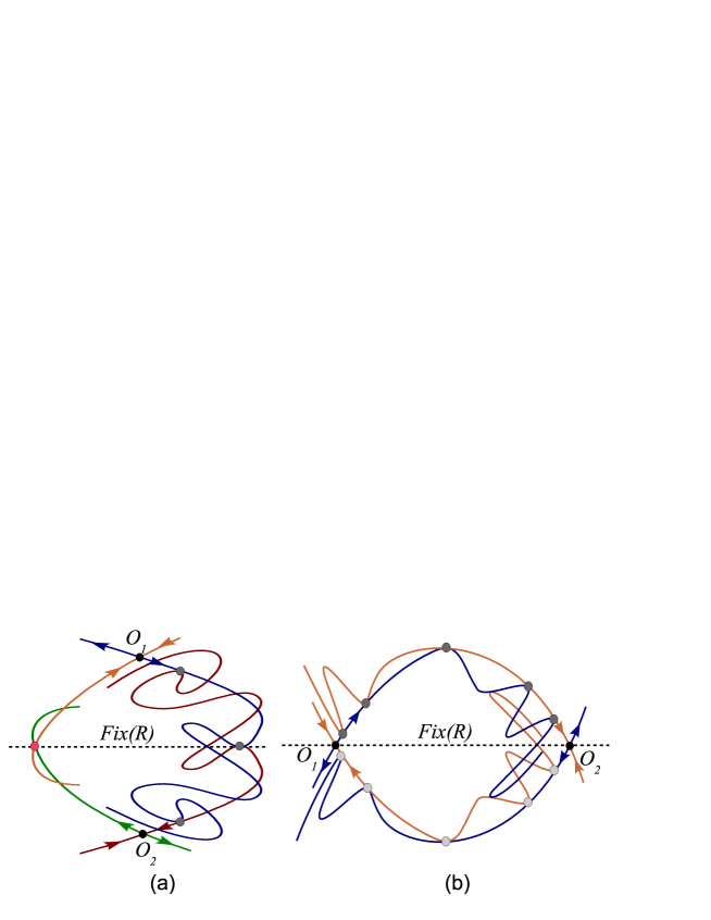
Figure 1: Two examples of planar reversible maps with symmetric non-transversal (quadratic tangency) heteroclinic cycles. One can think, for simplicity, that the involution $R$ in both cases is linear of form $x\mapsto x,y\mapsto-y$ and, thus, $\mbox{Fix}\;R=\{y=0\}$.

The above-mentioned mixed dynamics takes place as a generic phenomenon. This is the case, for instance, when the initial heteroclinic cycle is contracting-expanding [12], that is, when it contains contracting and expanding periodic points (i.e. with the absolute value of its Jacobian being greater or less than $1$). It is worth mentioning that contracting-expanding heteroclinic cycles are rather usual among reversible maps. An example of such a cycle is shown in Figure 1(a). In this example the reversible map has two saddle fixed points $O_{1}$ and $O_{2}$ and two heteroclinic orbits $\Gamma_{12}\subset W^{u}(O_{1})\cap W^{s}(O_{2})$ and $\Gamma_{21}\subset W^{u}(O_{2})\cap W^{s}(O_{1})$ such that $R(O_{1})=O_{2}$ and $R(\Gamma_{21})=\Gamma_{21}$, $R(\Gamma_{12})=\Gamma_{12}$. Besides, the orbit $\Gamma_{12}$ is non-transversal, so that the manifolds $W^{u}(O_{1})$ and $W^{s}(O_{2})$ have a quadratic tangency along $\Gamma_{12}$. Since $R(O_{1})=O_{2}$, it turns out that their Jacobians verify $J(O_{1})=J^{-1}(O_{2})$. If $J(O_{i})\neq\pm 1$, $i=1,2$, then the heteroclinic cycle is contracting-expanding. This condition is robust and is perfectly compatible with reversibility.

Certainly, results of [12] can be applied to reversible maps with such heteroclinic cycles and so the phenomenon of mixed dynamics becomes very important and generic. However, reversible systems are sharply different from general ones by the fact that they can possess robust non-hyperbolic symmetric periodic orbits, more precisely, elliptic symmetric periodic points. Thus, one realizes that the phenomenon of mixed dynamics in the case of two-dimensional reversible maps should be connected with the coexistence of infinitely many attracting, repelling, saddle and elliptic periodic orbits. The existence of Newhouse regions (intervals) in which this property is generic was already established in [23] for the case of reversible two-dimensional maps close to a map having a heteroclinic cycle of the type depicted in Figure 1(a).

However, it appears to be true that the phenomenon of mixed dynamics is universal for reversible (two-dimensional) maps with complicated dynamics when symmetric structures (symmetric periodic, homoclinic and heteroclinic orbits) are involved. This universality can be formulated as the following

Reversible Mixed Dynamics Conjecture  Two-dimensional reversible maps with mixed dynamics are generic (compose residual subsets) in Newhouse regions in which there are dense maps with symmetric homoclinic or/and heteroclinic tangencies.

We will assume, in what follows, that the involution $R$ is not trivial, i.e. it satisfies

$$R^{2}=\mbox{Id},\;\;\mbox{dim}\;\mbox{Fix}\;R=1.$$ (1.1)

We will say that an object $\Lambda$ is symmetric when $R(\Lambda)=\Lambda$. To put more emphasis, sometimes the notation self-symmetric may be used. By a symmetric couple of objects $\Lambda_{1},\Lambda_{2}$, we will mean two different objects that are symmetric to each other, i.e., $R(\Lambda_{1})=\Lambda_{2}$.

Then the symmetric homoclinic (heteroclinic) tangencies from the RMD-Conjecture can be divided into two main types: 1) there is a non-transversal symmetric heteroclinic orbit to a symmetric couple of saddle points, or 2) there is a symmetric couple of non-transversal homo/heteroclinic orbits to symmetric saddle points.

Notice that the heteroclinic quadratic tangency shown in Fig. 1(a) relates to the type 1), whereas an example of reversible map having a heteroclinic cycle of type 2) is shown in Figure 1(b). The latter map has two symmetric saddle fixed points $O_{1}$ and $O_{2}$ ($R(O_{1})=O_{1}$, $R(O_{2})=O_{2}$) and a symmetric couple of heteroclinic orbits $\Gamma_{12}\subset W^{u}(O_{1})\cap W^{s}(O_{2})$ and $\Gamma_{21}\subset W^{u}(O_{2})\cap W^{s}(O_{1})$ ($R(\Gamma_{12})=\Gamma_{21}$).

As we mentioned above, the case of non-transversal heteroclinic cycles of type 1), as in Fig. 1(a), was studied in the paper [23] where, in fact, the RMD-Conjecture was proved for general one-parameter (reversible) unfoldings, under the generic condition $J(O_{1})=J^{-1}(O_{2})\neq 1$.

In the first part of this paper, Sections 2 and 3, we state and prove the RMD-Conjecture for one-parameter families which unfold generally heteroclinic tangencies of type 2), as in Fig. 1(b). We will call this type as reversible maps with a symmetric couple of heteroclinic tangencies. We notice that in this case the condition $J(O_{1})=J(O_{2})=1$ holds always since $O_{i}\in\mbox{Fix}\;R$, showing that generic conditions are different in systems with different types. The generic condition that we are going to assume for systems of type 2) is denoted by condition [C] in Theorem 1. This condition (see (2.1) and comments to it) amounts to say that the (global) map defined near a heteroclinic point is neither a uniform contraction (expansion) nor a conservative map. More precisely, it has to have a non-constant Jacobian in those local coordinates (near $O_{1}$ and $O_{1}$) in which the saddle maps are, a priori, area-preserving. In particular, such local coordinates are given by Lemma 2 in which the normal form of the first order for a saddle map is derived.

Moreover, as we show, symmetry breaking bifurcations have also another nature, in comparison with [23]. We find a two-step “fold$\Rightarrow$pitch-fork” scenario of bifurcations in the first-return maps leading to the appearance of non-conservative fixed points which can be either attracting and repelling or saddle with Jacobian greater and less than $1$ (see Theorem 1 and Figure 4). Notice that in the case of heteroclinic cycles of type 1), such non-conservative points appear just under fold bifurcations [23] in a symmetric couple of first-return maps, whereas elliptic points appear in symmetric first-return maps.

The second part of this work, Section 4, has a more applied character. We show in Subsection 4.1 that reversible two-dimensional maps with a priori non-conservative orbit behaviour can be obtained as certain periodic perturbations of two-dimensional conservative flows of form $\dot{x}=y,\;\dot{y}=F(y)$ . We require that these perturbations include explicitly the “friction term” $\dot{x}$ and preserve only reversible properties of the initial flow (for example, they keep the perturbed systems to be invariant under the change $x\mapsto x,y\mapsto-y,t\mapsto-t$). In this way, in particular, we can obtain the reversible maps of type 2), see Figure 2. As a concrete example, we consider, in Subsection 4.1, the periodically perturbed Duffing equation. In Subsection 4.2 we consider an example of a reversible map from [30] defined on the two-dimensional torus which shows a visible non-conservative orbit behaviour. This map describes the dynamics of three coupled simple rotators with small symmetric couplings. The couplings are chosen here in such a way that they preserve the reversibility of the initial uncoupled three simple rotators.

In the third part of the paper, at Section 5, we consider a series of problems related to the representation of reversible two-dimensional maps in the so-called cross-form. It is well-known that such type of cross-forms of maps are very convenient for studying hyperbolic properties of systems with homoclinic orbits, both transversal [36] and non-transversal [6, 7, 21]. We show that the cross-forms and the corresponding cross-coordinates are natural for reversible maps, since they allow expressing many reversible structures explicitly and simplify analytical treatment. In particular, in the corresponding local cross-coordinates near a symmetric saddle periodic point, the normal form of the saddle map becomes very simple. And last (but not least), Section 6 contains the proofs of the lemmas needed in the proof of the main theorem 1.

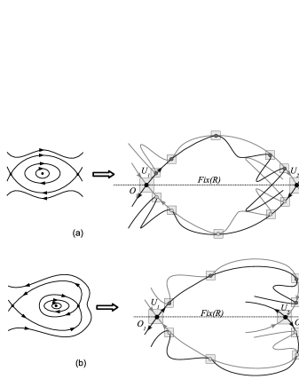
Figure 2: Examples of reversible maps with non-transversal heteroclinic cycles in the cases of (a) “inner tangency”; (b) “outer tangency”. These diffeomorphisms can be constructed as the Poincaré maps for periodically perturbed conservative planar systems (left) when the corresponding perturbations preserve the reversibility (for example, with respect to the change $x\to x,y\to-y,t\to-t$, as in the system $\dot{x}=y$, $\dot{y}=x-x^{3}+\varepsilon\dot{x}\cos t$). Notice that the resulting reversible map cannot be area-preserving, in general

1.1 Out of the general rule: a collection of reversible maps with codimension one homoclinic and heteroclinic tangencies

It is important to notice that there are many other cases of reversible maps with homoclinic and heteroclinic tangencies for which one needs to prove the RMD-Conjecture in the framework of one-parameter general families. In Figure 3 we collect some simple examples of such maps. They differ by the type of fixed points and tangencies: homoclinic or heteroclinic, quadratic or cubic, etc. However, it turns out to be more important that all this kind of maps could be separated into two groups: a first one including those maps which are a priori non-conservative and a second one with those maps where this non-conservativity is, in some sense, hidden.

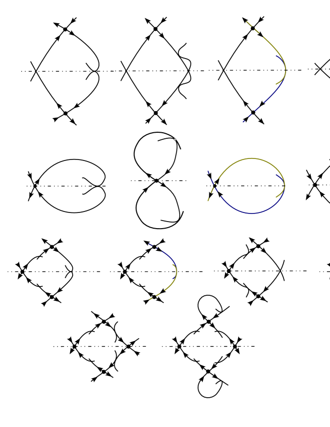
Figure 3: Some examples of reversible maps with homoclinic and heteroclinic tangencies

A map as in Figure 1(a) (the first one in Figure 3) belongs to the first group, since the condition $J(O_{1,2})\neq 1$ destroys certainly the conservative character. Indeed, under splitting such heteroclinic cycle, homoclinic tangencies appear both to saddles with Jacobian greater and less than 1 and, thus, attracting and repelling periodic points can be born [6]. By this principle, all the other cases where a symmetric couple of fixed (periodic) points are involved, can be referred to as the class of a priori non-conservative maps (e.g., all maps of the first, third and fourth rows of Figure 3). For maps of this type, the problem of finding symmetric periodic orbits (i.e., elliptic ones) has to be considered as very important.

The maps at the second row of Figure 3 have only symmetric fixed points. Evidently, the first, third and fourth maps can be assigned to maps with ”hidden non-conservativity”, since it is not clear, in advance, the existence of bifurcation mechanisms leading to the appearance of attracting and repelling periodic orbits. It is not the case of the third map (at the second row) which has a symmetric couple of (quadratic) homoclinic tangencies to the same symmetric fixed saddle point. One can assume, without loss of reversibility, that the map near a homoclinic point is not conservative (the Jacobian is greater or less than $1$). Then, clearly, stable (unstable) periodic orbits can be born under such homoclinic bifurcations. Thus, the main problem here is to prove the appearance of elliptic periodic orbits and, as a first step, to do it in the one-parameter setting.

1.2 A short description of the main results

We describe briefly the central ideas underlying our main results (Theorems 1 and 2). Let assume $f_{0}$ to be a $R$-reversible map of type as in Figure 1(b), that is, having two symmetric saddle fixed points $O_{1}$ and $O_{2}$ (i.e. $R(O_{i})=O_{i}$, $i=1,2$) and two asymmetric non-transversal heteroclinic orbits $\Gamma_{12}\subset W^{u}(O_{1})\cap W^{s}(O_{2})$ and $\Gamma_{21}\subset W^{u}(O_{2})\cap W^{s}(O_{1})$, satisfying that $R(\Gamma_{12})=\Gamma_{21}$. Let us consider $\left\{f_{\mu}\right\}$ any general one-parameter unfolding of $f_{0}$ with $\mu$ being the parameter splitting the initial heteroclinic tangency. The main goal of this paper is to show that under general hypotheses, any of these unfoldings undergoes infinitely many (in fact, a cascade) of symmetry-breaking bifurcations of single-round periodic orbits. Such bifurcations in these first-return maps (defined near some point of the heteroclinic tangency) follow from the following scenario:

$$\mbox{fold\;bifurcation}\;\;\Rightarrow\;\;\mbox{pitch-fork\; bifurcation}$$

Under fold-bifurcation, a symmetric parabolic fixed point appears which falls afterwards into two symmetric saddle and elliptic fixed points. Concerning (reversible) pitch-fork bifurcations, they can be of two classes depending essentially on the type of initial heteroclinic cycle they exhibit (see Figure 2 and 4): in case (a) we say that $f_{0}$ has a heteroclinic cycle of “inner tangency” while in case (b) we say that it is of “outer tangency”. In the first case, “inner tangency”, from the symmetric elliptic fixed point three fixed points are born: a symmetric saddle and asymmetric sink and source. In the second case, “outer tangency”, under a pitch-fork bifurcation, the symmetric saddle point becomes a symmetric elliptic point and two fixed asymmetric saddle points with Jacobian greater and less than 1. Both scenarios are showed in Figure 4. In the bifurcation diagram of Figure 8, related to a conservative approximation of the rescaled first-return map, value of $\tilde{c}<0$ corresponds to the “inner tangency” case and $\tilde{c}>0$ corresponds to the “outer tangency” one (situation $\tilde{c}=0$ is singular and not realisable for our maps; therefore there are no transitions from $\tilde{c}<0$ to $\tilde{c}>0$).

We finish this Introduction by describing the structure of the paper. Section 2 is devoted to the two above-mentioned main results of the paper, Theorems 1 and 2. Their proof is presented in Section 3 and relies to five lemmas whose proof is deferred to Sections 5, 6 and 6.3. Section 4 contains two concrete examples of applications of the main results of this paper.

2 Symmetry breaking bifurcations in the case of reversible maps with non-transversal heteroclinic cycles

Let $f_{0}$ be a $C^{r}$-smooth, $r\geq 4$, two-dimensional map, reversible with respect to an involution $R$ satisfying $\dim\;\mbox{Fix}(R)=1$. Let us assume that $f_{0}$ satisfies the following two conditions:

• $f_{0}$ has two saddle fixed points $O_{1}$ and $O_{2}$ belonging to the line $\mbox{Fix}(R)$ and that any point $O_{i}$ has multipliers $\lambda_{i},\lambda_{i}^{-1}$ with $0<\lambda_{i}<1$, $i=1,2$.

• The invariant manifolds $W^{u}(O_{1})$ and $W^{s}(O_{2})$ have quadratic tangencies at the points of some heteroclinic orbit $\Gamma_{12}$ and, therefore, by reversibility, the manifolds $W^{u}(O_{2})$ and $W^{s}(O_{1})$ have quadratic tangencies at the points of a heteroclinic orbit $\Gamma_{21}=R(\Gamma_{12})$.

Hypotheses [A]-[B] define reversible maps with non-transversal symmetric heteroclinic cycles like in Figure 1(b). We ask them to satisfy one more condition. Namely, consider two points $M_{1}\in W^{u}_{loc}(O_{1})$ and $M_{2}\in W^{s}_{loc}(O_{2})$ belonging to the same heteroclinic orbit $\Gamma_{12}$ and suppose $f_{0}^{q}(M_{1})=M_{2}$ for a suitable integer $q$. Let some smooth local coordinates $(x_{i},y_{i})$ be chosen near the points $O_{i}$ in such a way that the local invariant manifolds are straightened, i.e., $W^{u}_{loc}(O_{i})$ and $W^{s}_{loc}(O_{i})$ have, respectively, equations $x_{i}=0$ and $y_{i}=0$. Let $T_{12}$ denote the restriction of the map $f_{0}^{q}$ onto a small neighbourhood of the point $M_{1}$. Then, we assume that

• the Jacobian of $T_{12}$ is not constant and, moreover,

  $$Q=\frac{\partial J(T_{12})}{\partial y}\bigl{|}_{M_{1}}\neq 0$$ (2.1)

Condition $J(T_{12})\neq\;\mbox{const}$ is well defined only when certain restrictions on the local coordinates hold. One possibility is when these coordinates $(x_{i},y_{i})$ around $O_{i}$ are chosen in such a way that $W^{u}_{loc}(O_{1})$ and $W^{s}_{loc}(O_{2})$ are straightened. However, the sign of $J(T_{12})$ depends also on the orientation chosen for the coordinate axes. To be precise, we choose these orientations in such a a way that: $(i)$ the $y$ and $x-$coordinates of the heteroclinic points $M_{1}\in W^{u}_{loc}(O_{1})$ and $M_{2}\in W^{s}_{loc}(O_{2})$ are positive; $(ii)$ for the symmetric points, $M_{1}^{\prime}=R(M_{1})\in W^{s}_{loc}(O_{1})$ and $M_{2}^{\prime}=R(M_{2})\in W^{u}_{loc}(O_{2})$, the $x$ and $y$-coordinates are positive as well.

Two classes of reversible maps satisfying conditions [A]-[C] can be distinguished: those maps with “inner” (heteroclinic) tangency and those with “outer” tangency, corresponding to $J(T_{12})>0$ and $J(T_{12})<0$, respectively. Two examples of such diffeomorphisms are shown in Figure 2. Notice that in both cases the global map $T_{12}$ is orientable. In the case (a) the axes $x_{1},y_{1}$ and $x_{2},y_{2}$ have the same orientation, whereas the orientations are different in the case (b).

Once stated the general conditions for $f_{0}$, let us embed it into a one-parameter family $\left\{f_{\mu}\right\}$ of reversible maps that unfolds generally at $\mu=0$ the initial heteroclinic tangencies at the points of $\Gamma_{12}$. Then, without loss of generality, we can take $\mu$ as the corresponding splitting parameter. By reversibility, the invariant manifolds $W^{u}(O_{1})$ and $W^{s}(O_{2})$ split as $W^{u}(O_{2})$ and $W^{s}(O_{1})$ do when $\mu$ varies. Therefore, since these heteroclinic tangencies are quadratic, only one governing parameter is needed to control this splitting.

Let $U$ be an small enough neighbourhood of the contour $C=\{O_{1},O_{2},\Gamma_{12},\Gamma_{21}\}$. It can be represented as the union of two small neighbourhoods (disks) $U_{1}$ and $U_{2}$ of the saddles $O_{1}$ and $O_{2}$ and a finite number of small disks containing those points of $\Gamma_{12}$ and $\Gamma_{21}$ which do not belong to $U_{1}$ and $U_{2}$ (see Figure 2). We will focus our attention on the bifurcations of the so-called single-round periodic orbits, that is, orbits lying entirely in $U$ and having exactly one intersection point with every disk from the set $U\backslash(U_{1}\cup U_{2})$. Any point of a single-round periodic orbit is a fixed point of the corresponding first-return map $T_{km}$, that is constructed by orbits of $f_{\mu}$ with $k$ and $m$ iterations (of $f_{\mu}$) in $U_{1}$ and $U_{2}$, respectively. We will call them single-round periodic orbit of type $(k,m)$. The values of $k$ and $m$ will be always prescribed a priori. The first main result is as follows:

Theorem 1

Let $\left\{f_{\mu}\right\}_{\mu}$ be a one-parameter family of reversible diffeomorphisms that unfolds, generally, at $\mu=0$ the initial heteroclinic tangencies. Assume that $f_{0}$ verifies the conditions [A]-[C].

Then, at any segment $[-\epsilon,\epsilon]$ with $\epsilon>0$ , there are infinitely many intervals $\delta_{km}$ with border points $\mu_{\rm fold}^{(k,m)}$ and $\mu_{\rm pf}^{(k,m)}$ such that $\delta_{km}\to 0$ as $k,m\to\infty$ and the following holds:

• The value $\mu=\mu_{\rm fold}^{(k,m)}$ corresponds to a non-degenerate conservative fold bifurcation and, thus, the diffeomorphism $f_{\mu}$ has at $\mu\in\delta_{km}$ two symmetric, saddle and elliptic, single-round periodic orbits of type $(k,m)$.

• The value $\mu=\mu_{\rm pf}^{(k,m)}$ corresponds to a symmetric (and non-degenerate if condition [C] holds) pitch-fork bifurcation depending on the type of $f_{0}$:

  • In the case of “inner” tangency, single-round asymmetric attracting and repelling periodic orbits of type $(k,m)$ are born and, moreover, these orbits undergo simultaneously non-degenerate period doubling bifurcations at the value $\mu=\mu_{\rm pd}^{(k,m)}$ (where $\mu_{\rm pd}^{(k,m)}\to 0$ as $k,m\to\infty$).

  • For the “outer” tangency, two single-round saddle periodic orbits of type $(k,m)$ with Jacobian greater and less than $1$, respectively, are born. Moreover, they do not bifurcate any more (at least for $|\mu|<\epsilon$).

We refer the reader to Figure 4 for an illustration of this theorem.

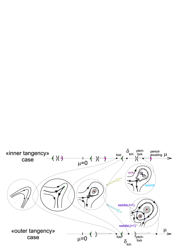
Figure 4: We mark, by shading, some intervals corresponding to the existence of two asymmetric single-round periodic orbits.

Theorem 1 and its counterpart result in [23] show that the appearance of non-conservative periodic orbits under global bifurcations can be consider as a certain generic property of two-dimensional reversible maps.

Briefly, the method we use - based on a rescaling technique - will allow us to prove that the first-return map $T_{km}$ can be written asymptotically close (as $k,m\to\infty$) to an area-preserving map of the form:

$$H\;:\left\{\begin{array}[]{l}\bar{x}=\tilde{M}+\tilde{c}x-y^{2},\\ \displaystyle\bar{y}=-\frac{\tilde{M}}{\tilde{c}}+\frac{1}{\tilde{c}}y+\frac{1}{\tilde{c}}(\tilde{M}+\tilde{c}x-y^{2})^{2},\end{array}\right.$$ (2.2)

in which the coordinates $(x,y)$ and the parameters $(\tilde{M},\tilde{c})$ can take arbitrary values except $\tilde{c}=0$. The region $\tilde{c}<0$ will stand for the “inner” tangency case and $\tilde{c}>0$ for the “outer” one. Its bifurcation diagram is showed in Figure 8. The map (2.2) is, in fact, the product of two Hénon maps with Jacobian $-\tilde{c}$ and $-\tilde{c}^{-1}$, (see equations (3.4)). Thus, we can state (see also [40]) that map (2.2) has a complicated dynamics in the corresponding parameter intervals. The latter means, in particular, that all fixed points become saddles and all of them have homoclinic and heteroclinic intersections for all values of the parameter $\mu$ including (quadratic) tangencies for dense subsets – Newhouse phenomenon.

An analogous “homoclinic tangle” can be observed for the first-return map $T_{km}$ (see Lemma 3). However, although the map (2.2) is reversible and conservative (its Jacobian is identically $1$), the original first-return map $T_{km}$ is also reversible but not conservative in general (see Lemma 4). Precisely, it will be shown that in some regions of the space of parameters $(\tilde{c},\tilde{M})$ the map $T_{km}$ possesses chaotic dynamics and has four saddle fixed points, two of them symmetric conservative and a symmetric couple of fixed points (that is, symmetric one to each other and with Jacobian greater and less than $1$, respectively). According to [12, 23, 20], the following result holds:

Theorem 2

Let $\left\{f_{\mu}\right\}$ be the one-parameter family of reversible maps from Theorem 1. Then, in any segment $[-\varepsilon,\varepsilon]$ of values of $\mu$, there are Newhouse intervals with mixed dynamics connected with an abundance of attracting, repelling and elliptic periodic orbits. This is, values of parameters corresponding to maps $f_{\mu}$ exhibiting simultaneously infinitely many periodic orbits of all these types form a residual set (of second category) in these intervals.

3 Proof of Theorem 1

3.1 Preliminary geometric and analytic constructions

To ease the reading all the proofs of the lemmas of this section have been deferred to Sections 5, 6 and 6.3.

Let us consider first the map $f_{0}$ and let $M_{1}^{-}\in U_{1}$, $M_{2}^{+}\in U_{2}$ be a pair of points of the orbit $\Gamma_{12}$ and $M_{2}^{-}\in U_{2}$, $M_{1}^{+}\in U_{1}$ be a pair of points of $\Gamma_{21}$. Consider $\Pi_{i}^{+}\subset U_{i}$ and $\Pi_{i}^{-}\subset U_{i}$ small neighbourhoods of the heteroclinic points $M_{i}^{+}$ and $M_{i}^{-}$ (see Figure 5). Let us assume that $(i)$ the heteroclinic points are symmetric under the involution $R$ , i.e. $M_{1}^{-}=R(M_{1}^{+})$ and $M_{2}^{-}=R(M_{2}^{+})$, and $(ii)$ they are the “last” points on $U_{1}$ and $U_{2}$, that is, $f_{0}(M_{i}^{-})\notin U_{i}$ (and, thus, $f_{0}^{-1}(M_{i}^{+})\notin U_{i}$). Let $q$ be such an positive integer that $M_{2}^{+}=f_{0}^{q}(M_{1}^{-})$ (and, thus, $M_{1}^{+}=f_{0}^{q}(M_{2}^{-})$).

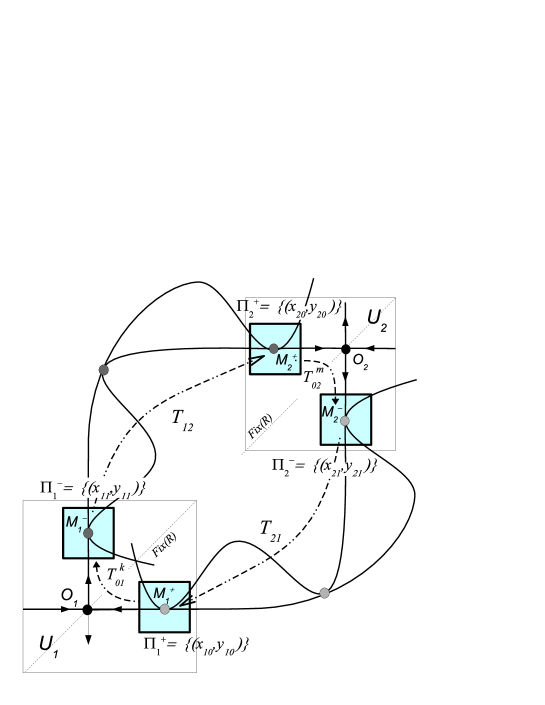
Figure 5: Schematic actions of the local ($T_{01}^{k}$ and $T_{02}^{m}$) and global ($T_{12}$ and $T_{21}$) maps in the neighbourhood $U$ of the contour $C=\{O_{1},O_{2},\Gamma_{12},\Gamma_{21}\}$.

Consider now the map $f_{\mu}$. Denote $T_{0i}\equiv{f_{\mu}}\bigl{|}_{U_{i}}$, $i=1,2$. The maps $T_{01}$ and $T_{02}$ are called the local maps. We introduce also the so-called global maps $T_{12}$ and $T_{21}$ by the following relations: $T_{12}\equiv f^{q}_{\mu}:\Pi_{1}^{-}\to\Pi_{2}^{+}$ and $T_{12}\equiv f^{q}_{\mu}:\Pi_{2}^{-}\to\Pi_{1}^{+}$ (see Figure 5). Then the first-return map $T_{km}:\Pi_{1}^{+}\mapsto\Pi_{1}^{+}$ is defined by the following composition of maps and neighbourhoods:

$$\Pi_{1}^{+}\;\stackrel{{\scriptstyle T_{01}^{k}}}{{\longrightarrow}}\;\;\Pi_{1}^{-}\;\stackrel{{\scriptstyle T_{12}}}{{\longrightarrow}}\;\;\Pi_{2}^{+}\;\stackrel{{\scriptstyle T_{02}^{m}}}{{\longrightarrow}}\;\;\Pi_{2}^{-}\;\stackrel{{\scriptstyle T_{21}}}{{\longrightarrow}}\;\;\Pi_{1}^{+}$$ (3.1)

Denote local coordinates on $\Pi_{i}^{+}$ and $\Pi_{i}^{-}$ as $(x_{0i},y_{0i})$ and $(x_{1i},y_{1i})$, respectively. Then the chain (3.1) can be represented (in coordinates) as

$$(x_{01},y_{01})\stackrel{{\scriptstyle T_{01}^{k}}}{{\longmapsto}}(x_{11},y_{11})\stackrel{{\scriptstyle T_{12}}}{{\longmapsto}}(x_{02},y_{02})\stackrel{{\scriptstyle T_{02}^{m}}}{{\longmapsto}}(x_{12},y_{12})\stackrel{{\scriptstyle T_{21}}}{{\longmapsto}}(\bar{x}_{01},\bar{y}_{01}).$$

As usually, we need such local coordinates on $U_{1}$ and $U_{2}$ in which the maps $T_{01}$ and $T_{02}$ have their simplest form. We can not assume the maps $T_{0i}$ are linear, since by condition [A], only $C^{1}$-linearisation is possible here. Therefore, we consider such $C^{r-1}$-coordinates in which the local maps have the so-called main normal form or normal form of the first order.

Lemma 1 (Main normal form of a saddle map)

Let a $C^{r}$-smooth map $T_{0}$ be reversible with $\dim\mbox{Fix}(T_{0})=1$. Suppose that $T_{0}$ has a saddle fixed (periodic) point $O$ belonging to the line $\mbox{Fix}(T_{0})$ and having multipliers $\lambda$ and $\lambda^{-1}$, with $|\lambda|<1$. Then there exist $C^{r-1}$-smooth local coordinates near $O$ in which the map $T_{0}$ (or $T_{0}^{n}$, where $n$ is the period of $O$) can be written in the following form:

$$T_{0}:\;\;\begin{array}[]{l}\bar{x}=\lambda x(1+h_{1}(x,y)xy)\\ \bar{y}=\lambda^{-1}y(1+h_{2}(x,y)xy),\end{array}$$ (3.2)

where $h_{1}(0)=-h_{2}(0)$. The map (3.2) is reversible with respect to the standard linear involution $(x,y)\mapsto(y,x)$.

When proving this lemma one can deduce more “descriptive” properties of this map. Namely, one can show that it could be written in the so-called cross-form (see Section 5.1) as follows:

$$T_{0}:\;\;\begin{array}[]{l}\bar{x}=\lambda x+\hat{h}(x,\bar{y})x^{2}\bar{y},\\ y=\lambda\bar{y}+\hat{h}(\bar{y},x)x\bar{y}^{2}.\end{array}$$ (3.3)

Notice that when $T_{0}$ is linear, i.e. $T_{0}:\;\bar{x}=\lambda x,\bar{y}=\lambda^{-1}y$, one can easyly find formulas for its iterates $T_{0}^{j}$, $j\in\mathbb{Z}$. Namely, one can write it either as $x_{j}\lambda^{j}x_{0},y_{j}=\lambda^{-j}y_{0}$ or, in cross-form, as $x_{j}=\lambda^{j}x_{0},y_{0}=\lambda^{j}y_{j}$. If $T_{0}$ is non-linear, then its cross-form equations exist too. In particular, the following result holds:

Lemma 2 (Iterations of the local map)

Let $T_{0}$ be a saddle map written in the main normal form (3.2) (or (3.3)) in a small neighbourhood $V$ of $O$. Let us consider points $(x_{0},y_{0}),\dots,(x_{j},y_{j})$ from $V$ such that $(x_{l+1},y_{l+1})=T_{0}(x_{l},y_{l})$, $l=0,\dots,j-1$. Then one has

$$x_{j} = \lambda^{j}x_{0}\left(1+j\lambda^{j}h_{j}(x_{0},y_{j})\right),$$ (3.4)

$$y_{0} = \lambda^{j}y_{j}\left(1+j\lambda^{j}h_{j}(y_{j},x_{0})\right),$$

where the functions $h_{j}(y_{j},x_{0})$ are uniformly bounded with respect to $j$ as well all their derivatives up to order $r-2$.

Remark 1

• Both lemmas 1 and 2 remain true if $T_{0}$ depends on parameters. Moreover, if the initial $T_{0}$ is $C^{r}$ with respect to coordinates and parameters, then the normal form (3.2) is $C^{r-1}$ with respect to coordinates and $C^{r-2}$ with respect to parameters (see [20]).

• It follows from Lemma 1 that the involution $L(x,y)=(y,x)$ is very convenient for the construction of symmetric saddle maps. Moreover, this involution is (locally) smoothly equivalent to any other involution $R$ with $\dim\;\mbox{Fix}(R)=1$ (see [24]). Thus, our assumption on a concrete form of the involution for the maps $f_{\mu}$ does not lead to loss of generality.

• Similar results related to finite-smooth normal forms of saddle maps were established in [8, 14, 17, 20] for general, near-conservative and conservative maps. In this paper we, in fact, modify the corresponding proofs adapting them to the reversible case.

3.2 Construction of the local and global maps

By Lemma 2, we can choose in $U_{1}$ and $U_{2}$ local coordinates $(x_{1},y_{1})$ and $(x_{2},y_{2})$, respectively, such that the maps $T_{01}$ and $T_{02}$ take the following form:

$$T_{01}:\;\;\bar{x}_{1}=\lambda_{1}x_{1}+h_{1}^{1}(x_{1},y_{1})x_{1}^{2}y_{1},\quad\bar{y}_{1}=\lambda_{1}^{-1}y_{1}+h_{2}^{1}(x_{1},y_{1})x_{1}y_{1}^{2},$$

and

$$T_{02}:\;\;\bar{x}_{2}=\lambda_{2}x_{2}+h_{1}^{2}(x_{2},y_{2})x_{2}^{2}y_{2},\quad\bar{y}_{2}=\lambda_{2}^{-1}y_{2}+h_{2}^{2}(x_{2},y_{2})x_{2}y_{2}^{2}.$$

Furthermore, in these coordinates, the local stable and unstable invariant manifolds of both points $O_{1}$ and $O_{2}$ are straightened: $x_{i}=0$ is the equation of $W^{u}_{loc}(O_{i})$ and $y_{i}=0$ is the equation of $W^{s}_{loc}(O_{i})$, $i=1,2$. Then, we can write the $(x,y)$-coordinates of the chosen heteroclinic points as follows: $M_{1}^{+}(x_{1}^{+},0)$, $M_{1}^{-}(0,y_{1}^{-})$, $M_{2}^{+}(x_{2}^{+},0)$ and $M_{2}^{-}(0,y_{2}^{-})$. Besides, because of the reversibility, we have that

$$x_{1}^{+}=y_{1}^{-}=\alpha_{1}^{*},\qquad x_{2}^{+}=y_{2}^{-}=\alpha_{2}^{*}$$ (3.5)

We assume that $T_{0i}(\Pi_{i}^{+})\cap\Pi_{i}^{+}=\emptyset$ and $T_{0i}^{-1}(\Pi_{i}^{-})\cap\Pi_{i}^{-}=\emptyset$, $i=1,2$. Then the domain of definition of the successor map from $\Pi_{i}^{+}$ into $\Pi_{i}^{-}$ under iterations of $T_{0i}$ consists of infinitely many non-intersecting strips $\sigma_{j}^{0i}$ which belong to $\Pi_{i}^{+}$ and accumulate at $W^{s}_{loc}(O_{i})\cap\Pi_{i}^{+}$ as $j\to\infty$. Analogously, the range of this map consists of infinitely many strips $\sigma_{j}^{1i}=T_{0i}^{j}(\sigma_{j}^{0i})$ belonging to $\Pi_{i}^{-}$ and accumulating at $W^{u}_{loc}(O_{i})\cap\Pi_{i}^{-}$ as $j\to\infty$ (see Figure 6).

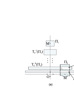
Figure 6: A geometry of creation of both domains of definition $\sigma_{i}^{0}\subset\Pi^{+}$ (a) and domains of the range $\sigma_{i}^{1}\subset\Pi^{-}$ (b) for the maps $T_{0}^{i}:\Pi^{+}\to\Pi^{-}$.

It follows from Lemma 2 that the map $T_{01}^{k}:\sigma_{k}^{01}\mapsto\sigma_{k}^{11}$ can be written in the following form (for large enough values of $k$)

$$T_{01}^{k}\;:\;\left\{\begin{array}[]{l}x_{11}=\lambda_{1}^{k}x_{01}(1+k\lambda_{1}^{k}h_{k}^{1}(x_{01},y_{11}))\\ y_{01}=\lambda_{1}^{k}y_{11}(1+k\lambda_{1}^{k}h_{k}^{1}(y_{11},x_{01}))\end{array}\right.$$ (3.6)

and an analogous formula takes place for the map $T_{02}^{m}:\sigma_{m}^{02}\mapsto\sigma_{m}^{12}$:

$$T_{02}^{m}:\;\left\{\begin{array}[]{l}x_{12}=\lambda_{2}^{m}x_{02}(1+m\lambda_{2}^{m}h_{m}^{2}(x_{02},y_{12}))\\ y_{02}=\lambda_{2}^{m}y_{12}(1+m\lambda_{2}^{m}h_{m}^{2}(y_{12},x_{02}))\end{array}\right.$$

We write now the global map $T_{12}$ in the following form

$$\!T_{12}\left\{\begin{array}[]{l}x_{02}-x_{2}^{+}=F_{12}(x_{11},y_{11}-y_{1}^{-},\mu)\equiv ax_{11}+b(y_{11}-y_{1}^{-})+\\ \qquad\qquad l_{02}(y_{11}-y_{1}^{-})^{2}+\varphi_{1}(x_{11},y_{11},\mu),\\ y_{02}=G_{12}(x_{11},y_{11}-y_{1}^{-},\mu)\equiv\mu+cx_{11}+d(y_{11}-y_{1}^{-})^{2}+\\ \qquad\qquad f_{11}x_{11}(y_{11}-y_{1}^{-})+f_{03}(y_{11}-y_{1}^{-})^{3}+\\ \qquad\qquad\varphi_{2}(x_{11},y_{11},\mu),\end{array}\right.$$ (3.7)

where $F_{12}(0)=G_{12}(0)=0$ since $T_{12}(M_{1}^{-})=M_{2}^{+}$ at $\mu=0$ and

$$\begin{array}[]{l}\varphi_{1}=O(|y_{11}-y_{1}^{-}|^{3})+x_{11}O(\|(x_{11},y_{11}-y_{1}^{-})\|),\\ \varphi_{2}=O(|x_{11}|^{2})+O(|y_{11}-y_{1}^{-}|^{4})+O(x_{11}(y_{11}-y_{1}^{-})^{2}).\end{array}$$

Since the curves $T_{12}\left(W^{u}_{loc}(O_{1}):\{x_{11}=0\}\right)$ and $W^{s}_{loc}(O_{2}):\{y_{02}=0\}$ have a quadratic tangency at $\mu=0$, it implies that

$$\frac{\partial G_{12}(0)}{\partial y_{11}}=0,\;\;\frac{\partial^{2}G_{12}(0)}{\partial y_{11}^{2}}=2d\neq 0.$$

The Jacobian $J(T_{12})$ has, obviously, the following form:

$$J(T_{12})=-bc+af_{11}x_{11}+Q\;(y_{11}-y_{1}^{-})+O\left(x_{11}^{2}+(y_{11}-y_{1}^{-})^{2}\right),$$

where

$$Q=2ad-bf_{11}-2cl_{02}.$$ (3.8)

Now condition [C] can be formulated more precisely. Namely, we require that

$$Q\;=\;\frac{\partial J(T_{12})}{\partial y_{11}}{\Bigl{|}_{{(x_{11}=0,y_{11}=y_{1}^{-},\mu=0)}}}\;\neq\;0$$

Concerning the global map $T_{21}$, we cannot write it now in an arbitrary form. The point is that after written a formula for the map $T_{12}$ it is necessary to use the reversibility relations to get the one associated to it:

$$T_{21}=R\;T_{12}^{-1}\;R^{-1},\qquad T_{12}=R\;T_{21}^{-1}\;R^{-1}$$

for constructing $T_{21}$. Then, by (3.7), we obtain that the map $T_{21}^{-1}:\Pi_{1}^{+}\{(x_{01},y_{01})\}\mapsto\Pi_{2}^{-}\{(x_{12},y_{12})\}$ must be written as follows

$$\!T_{21}^{-1}\left\{\begin{array}[]{l}x_{12}=G_{12}(y_{01},x_{01}-y_{1}^{-},\mu)=\\ \quad\mu+cy_{01}+d(x_{01}-y_{1}^{-})^{2}+f_{11}y_{01}(x_{01}-y_{1}^{-})+\\ \quad f_{13}(x_{01}-y_{1}^{-})^{2}+\varphi_{2}(y_{01},x_{01},\mu),\\ y_{12}-x_{2}^{+}=F_{12}(y_{01},x_{01}-y_{1}^{-},\mu)=\\ \quad ay_{01}+b(x_{01}-y_{1}^{-})+l_{02}(x_{01}-y_{1}^{-})^{2}+\varphi_{1}(y_{01},x_{01},\mu)\\ \end{array}\right.$$ (3.9)

Relation (3.9) allows to define the map $T_{21}:\Pi_{2}^{-}\{(x_{12},y_{12})\}\mapsto\Pi_{1}^{+}\{(x_{01},y_{01})\}$, but in implicit form.

3.3 Construction of the first-return maps $T_{km}$ and the Rescaling Lemma

Now, using relations (3.6)–(3.9), we can construct the first-return map $T_{km}=T_{21}T_{02}^{m}T_{12}T_{01}^{k}$ defined on the strip $\sigma_{k}^{01}\subset\Pi^{+}_{1}$. Recall that any fixed point of $T_{km}$ corresponds to a single-round periodic orbit of type $(k,m)$ of period $(k+m+2q)$. However, we do not state the problem of studying the maps $T_{km}$ for all large $k$ and $m$. We suppose $k$ and $m$ are large enough integers such that

$$\lambda_{1}^{k}\simeq\lambda_{2}^{m}.$$ (3.10)

In other words, both values of $\lambda_{1}^{k}\lambda_{2}^{-m}$ and $\lambda_{1}^{-k}\lambda_{2}^{m}$ are uniformly separated from $0$ and $\infty$ as $k,m\to\infty$. Then the following result holds.

Lemma 3 (The rescaling lemma)

Let the map $f_{0}$ satisfy conditions [A]-[B] and $f_{\mu}$ be a general unfolding in the class of reversible maps. Suppose $k$ and $m$ are large enough integer numbers satisfying relation (3.10). Then one can introduce coordinates (called “rescaled coordinates”) in such a way that the first-return map $T_{km}$ takes the form

$$\begin{array}[]{l}M+c\bar{y}+d\bar{x}^{2}+f_{11}\lambda_{1}^{k}\bar{x}\bar{y}+f_{03}\lambda_{1}^{k}\bar{x}^{3}=\\ \qquad=b\lambda_{2}^{m}\lambda_{1}^{-k}y+a\lambda_{2}^{m}x+l_{02}\lambda_{2}^{m}y^{2}+O(k\lambda_{1}^{2k}),\\ \\ M+cx+dy^{2}+f_{11}\lambda_{1}^{k}xy+f_{03}\lambda_{1}^{k}y^{3}=\\ \qquad b\lambda_{2}^{m}\lambda_{1}^{-k}\bar{x}+a\lambda_{2}^{m}\bar{y}+l_{02}\lambda_{2}^{m}\bar{x}^{2}+O(k\lambda_{1}^{2k}),\end{array}$$ (3.11)

where

$$M=\lambda_{1}^{-2k}\left(\mu+c\lambda_{1}^{k}\alpha_{1}^{*}(1+\dots)-\lambda_{2}^{m}\alpha_{2}^{*}(1+\dots)\right)$$ (3.12)

and “$\ldots$” stands for some coefficients tending to zero as $k,m\to\infty$. Notice that the domain of definition of the new coordinates $x\sim\lambda_{1}^{-k}(x_{01}-\alpha_{1}^{*})$, $y\sim\lambda_{1}^{-k}(y_{11}-\alpha_{1}^{*})$ and parameter $M$ cover all finite values as $k,m\to\infty$.

3.4 On bifurcations of fixed points of the first-return maps $T_{km}$

We study bifurcations in the first-return map $T_{km}$ using its rescaled form (3.11). If we neglect in (3.11) all asymptotically small terms (as $k,m\to\infty$), we obtain the following truncated form for $T_{km}$

$$\begin{array}[]{l}M+c\bar{y}+d\bar{x}^{2}=\beta_{km}y,\;\;\beta_{km}\bar{x}=M+cx+dy^{2},\end{array}$$ (3.13)

where $\beta_{km}=b\lambda_{1}^{-k}\lambda_{2}^{m}$. Rescale the coordinates

$$x\;=\;-\frac{\beta_{km}}{d}x_{new},\;\;y\;=\;-\frac{\beta_{km}}{d}y_{new}.$$

Then map (3.13) is rewritten in the following form, that we denote with $H$:

$$H:\ \ \tilde{M}+\tilde{c}\bar{y}-\bar{x}^{2}=y,\qquad\bar{x}=\tilde{M}+\tilde{c}x-y^{2},$$ (3.14)

where

$$\tilde{M}=-\frac{d}{\beta_{km}^{2}}\;M,\;\;\tilde{c}=\frac{1}{\beta_{km}}\equiv\frac{c}{b}\lambda_{1}^{k}\lambda_{2}^{-m}\;$$ (3.15)

Notice that $H$ depends on two parameters $\tilde{M}$ and $\tilde{c}$ which can take arbitrary values, except for $\tilde{c}=0$ (according to conditions $bc\neq 0$ and $0<|\lambda_{i}|<0$). Thus, two mainly different scenarios take place: with $\tilde{c}<0$ and $\tilde{c}>0$.

Observe that the map $H$ can be expressed in the explicit form (2.2). Moreover, it can be represented as the superposition $H=\mathcal{H}_{2}\circ\mathcal{H}_{1}$ of two quadratic (Hénon) maps

$$\begin{array}[]{l}\mathcal{H}_{1}:\{\;\;x_{1}=y_{0},\qquad y_{1}=\tilde{M}+\tilde{c}x_{0}-y_{0}^{2},\\ \displaystyle\mathcal{H}_{2}:\{\;\;x_{2}=y_{1},\qquad y_{2}=-\frac{\tilde{M}}{\tilde{c}}+\frac{1}{\tilde{c}}x_{1}+\frac{1}{\tilde{c}}y_{1}^{2}.\end{array}$$

The Jacobians of these maps are constant and inverse: $J(\mathcal{H}_{1})=-\tilde{c}$ and $J(\mathcal{H}_{2})=-\tilde{c}^{-1}$. Therefore, the resulting map $H=\mathcal{H}_{2}\circ\mathcal{H}_{1}$ is a quadratic map with the Jacobian equal to $1$ and so area-preserving.

Form (3.14) of $H$ allows to give a rather simple geometric interpretation of the bifurcations of fixed points. The coordinates $(x,y)$ of these fixed points must satisfy the equations

$$y(1-\tilde{c})=\tilde{M}-x^{2},\qquad x(1-\tilde{c})=\tilde{M}-y^{2}$$ (3.16)

Let us hold fixed $\tilde{c}$ and suppose that $\tilde{c}\neq 1$. Then equations of (3.16) define on the $(x,y)$-plane two parabolas which are symmetric with respect to the bisectrix $y=x$. Intersection points of the parabolas are also fixed points of $H$. When $\tilde{M}$ varies the parabolas “move” and, as a result, the number of intersection points can change (i.e. bifurcations in $H$ occur). See Figure 7 in which the case $\tilde{c}<1$ is illustrated: (a) the parabolas do not intersect if $\tilde{M}<M_{1}^{*}\equiv-\frac{1}{4}(\tilde{c}-1)^{2}$; (b) the parabolas are touched (quadratically) to the bisectrix and one to other, if $\tilde{M}=M_{1}^{*}$; (c) they have two (symmetric) intersection points if $M_{1}^{*}<\tilde{M}<M_{2}^{*}\equiv\frac{3}{4}(\tilde{c}-1)^{2}$; (d) they have a cubic (symmetric) tangency when $\tilde{M}=M_{2}^{*}$ and, finally, (e) the parabolas have four intersection points (two symmetric points and a symmetric couple of points) if $\tilde{M}>M_{2}^{*}$.

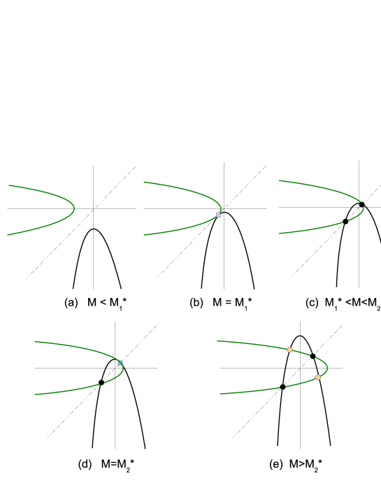
Figure 7: A geometric interpretation for a structure of fixed points of map (3.14) as intersection points of two symmetric parabolas.

An analogous picture takes place for the case $\tilde{c}>1$ (the parabolas have their branches in the opposite directions). The case $\tilde{c}=1$ is very special. Here, the equation (3.16) takes the form $0=\tilde{M}-x^{2},0=\tilde{M}-y^{2}$ and, thus, a certain $"0-4"$-bifurcation occurs at $\tilde{M}=0$: the map $H$ has no fixed points for $\tilde{M}<0$ and 4 fixed points appear immediately when $\tilde{M}$ becomes positive.

More details concerning bifurcations of fixed points of $H$ are illustrated in Figure 8 where principal elements of the bifurcation diagram on the $(\tilde{c},\tilde{M})$-plane are represented. Notice that the line $\tilde{c}=0$ is singular and, therefore, there are no transitions between the half-planes $\tilde{c}<0$ and $\tilde{c}>0$. In particular, this means that bifurcation curves must “terminate” on the line $\tilde{c}=0$ (two such terminated points are denoted in Figure 8 as black stars). Besides, three types of bifurcation curves are represented in the figure: fold ($F$), period-doubling ($PD$) and pitch-fork ($PF$).

The curves $\mbox{F}_{1}$ and $\mbox{F}_{2}$ having the same equation

$$\tilde{M}=-\frac{1}{4}(\tilde{c}-1)^{2}$$ (3.17)

but with $\tilde{c}<0$ and $\tilde{c}>0$, respectively, relate to a conservative fold-bifurcation. If $\tilde{M}<-\frac{1}{4}(\tilde{c}-1)^{2}$, i.e. $(\tilde{c},\tilde{M})\in I_{l}\cup I_{r}$, the map $H$ has no fixed points; if $\tilde{M}>-\frac{1}{4}(\tilde{c}-1)^{2}$, the map $H$ has two symmetric fixed points $P^{+}=(p_{+},p_{+})$ and $P^{-}=(p_{-},p_{-})$, where

$$p^{\pm}=\frac{\tilde{c}-1\pm\sqrt{(\tilde{c}-1)^{2}+4\tilde{M}}}{2}.\tilde{M}=-\frac{1}{4}(\tilde{c}-1)^{2}$$ (3.18)

Notice that the point $Q^{*}=(\tilde{c}=1,\tilde{M}=0)\in\mbox{F}_{2}$ corresponds to a degenerate fold-bifurcation: simultaneously four fixed points, two symmetric and a symmetric couple, are born at the transition $\mbox{I}_{r}\rightarrow\mbox{V}_{r}$.

In the case $\tilde{c}<0$, the point $p_{-}$ is always a saddle and it does not bifurcate any more. This is not the case of the point $p_{+}$ which can undergo both period-doubling and pitch-fork bifurcations. The period-doubling bifurcation curves

$$\begin{array}[]{l}\displaystyle PD^{1}(p_{+}):\;\;\tilde{M}=1-\frac{1}{4}(\tilde{c}-1)^{2},\;\;\tilde{c}<0;\\ \displaystyle PD^{2}(p_{+}):\;\;\tilde{M}=\frac{(c+1)(3c-1)}{4},\;\;\tilde{c}<0.\end{array}$$

are represented in Figure 8 by “grey arrows” which indicate directions of birth of period-$2$ points. The curve

$$\begin{array}[]{l}PF^{1}(p_{+}):\;\;\tilde{M}=\frac{3}{4}(\tilde{c}-1)^{2},\;\;\tilde{c}<0\\ \end{array}$$

relates to the pitch-fork bifurcation: when crossing this curve (in the direction $\mbox{V}_{l}\rightarrow\mbox{VI}_{l}$) the point $p_{+}$ becomes saddle and two asymmetric elliptic fixed points $p_{3}$ and $p_{4}$ are born in its neighbourhood. The point $p_{+}$ does not bifurcate any more, whereas, the points $p_{3}$ and $p_{4}$ undergo simultaneously period-doubling bifurcation at crossing the curve

$$PD(p_{3,4}):\;\;\tilde{M}=\frac{(1-3\tilde{c})(3-\tilde{c})}{4},\quad\tilde{c}<0$$

Further variation of parameters in the domain $\mbox{VII}_{l}$, will lead to a cascade of (conservative) period-doubling bifurcations of asymmetric periodic points.

Figure 8: Elements of the bifurcation diagram for the map $H$.

As it can be seen in Figure 8, the character of the bifurcations in the case $\tilde{c}>0$ is different to the one for $\tilde{c}<0$. In this case, $\tilde{c}>0$, both symmetric fixed points $p_{+}$ and $p_{-}$ undergo pitch-fork and period-doubling bifurcations. The corresponding bifurcation curves are

$$\begin{array}[]{l}\displaystyle PF^{2}(p_{+}):\quad\tilde{M}=\frac{3}{4}(\tilde{c}-1)^{2},\;\;0<\tilde{c}<1;\\ \displaystyle PD^{3}(p_{+}):\quad\tilde{M}=1-\frac{1}{4}(\tilde{c}-1)^{2},\quad\tilde{c}>0;\\ \end{array}$$

for the point $p_{+}$ and

$$\begin{array}[]{l}\displaystyle PF(p_{-}):\quad\tilde{M}=\frac{3}{4}(\tilde{c}-1)^{2},\quad\tilde{c}>1;\\[5.16663pt] \displaystyle PD(p_{-}):\quad\tilde{M}=\frac{(c+1)(3c-1)}{4},\quad\tilde{c}>0\\ \end{array}$$ (3.19)

for the point $p_{-}$. Notice that, when crossing the curve $PF^{2}(p_{+})\cup PF(p_{-})$, a symmetric couple of saddle fixed points $p_{3}$ and $p_{4}$ are born and they do not bifurcate any more (for values of parameters $\tilde{c}>0$ and $\tilde{M}$ in the domain lying above the curve $PF^{2}(p_{+})\cup PF(p_{-})$). One can expect, however, that bifurcations of the symmetric fixed points $p_{+}$ and $p_{-}$ give rise to cascades of period-doubling bifurcations.

It should be noted that, despite the reversibility, the pitch-fork and period-doubling bifurcations can have in $T_{km}$ a different character in comparison with the one of the truncated map $H$. Of course, the pitch-fork bifurcation in $T_{km}$ leads again to the appearance of two non-symmetric fixed points $p_{3}$ and $p_{4}$ but these points can be non-conservative. In fact, this is a general property (it holds for open and dense set of systems) that the following lemma shows.

Lemma 4 (Non-conservative fixed points)

The non-symmetric fixed points $p_{3}$ and $p_{4}$ of map (3.11), with $k$ and $m$ satisfying (3.10), have Jacobian $J_{ns}$ and $J_{ns}^{-1}$, respectively, with

$$J_{ns}=1+\frac{Q(\eta^{*}-\xi^{*})}{bc}\lambda_{1}^{k}+o(\lambda_{1}^{k}),$$ (3.20)

where $Q$ is the coefficient given by formula (3.8) and $\xi^{*}$ and $\eta^{*}$ are, respectively, the $x$- and $y$-coordinate of the fixed point.

Due to the reversibility, the fold bifurcation in the first-return map $T_{km}$ has the same character as in the truncated map $H$ and leads, therefore, to the appearance of two symmetric fixed points, $p_{+}$ and $p_{-}$, saddle and elliptic ones. Concerning the symmetric elliptic fixed points, we have the following result.

Lemma 5 (Symmetric elliptic fixed points)

The point $p_{+}$ (resp. the point $p_{-}$) is generic elliptic, that is, it is KAM-stable, for open and dense sets of values of the parameters $(\tilde{c},\tilde{M})$ in the domains $\mbox{II}_{l}\cup\mbox{V}_{l}$ and $\mbox{IV}_{r}\cup\mbox{V}_{r}\cup\mbox{VI}_{r}$ (resp. in the domain $\mbox{II}_{r}\cup\mbox{V}_{r}\cup\mbox{VIII}_{r}$).

The proofs of lemmas 3–5 are given in Section 6.3.

3.5 End of the proof of Theorem 1.

If $k$ and $m$ are large enough and having in mind (3.10), (3.12) and (3.15), the following relation between the parameters $\mu$ and $\tilde{M}$ holds:

$$\mu=\lambda_{2}^{m}\alpha_{2}^{*}(1+\rho_{k}^{1})-c\lambda_{1}^{k}\alpha_{1}^{*}(1+\rho_{k}^{2})-\frac{b^{2}}{d}\tilde{M}\lambda_{2}^{2m}(1+\rho_{k}^{3}),$$

where $\rho_{k}^{i},i=1,2,3,$ are some small coefficients ($\rho_{k}^{i}\to 0$ as $k\to\infty$). Using formulas (3.17)–(3.19) for the bifurcation curves of the truncated map (3.14), asymptotically close to the (rescaled) first-return map (3.11), we find the following expressions for the bifurcation values of $\mu$ at the statement of Theorem 1: a value $\mu=\mu_{\rm fold}^{(k,m)}$, which corresponds to the fold bifurcation in $T_{km}$,

$$\mu_{\rm fold}^{(k,m)} = \lambda_{2}^{m}\alpha_{2}^{*}(1+\rho_{k}^{1})-c\lambda_{1}^{k}\alpha_{1}^{*}(1+\rho_{k}^{2})+$$

$$\frac{1}{4d}(b-c\lambda_{1}^{k}\lambda_{2}^{m})^{2}\lambda_{2}^{2m}(1+\rho_{k}^{3})$$

and a value $\mu=\mu_{pf}^{(k,m)}$, associated to the pitch-fork bifurcation in $T_{km}$ (which is not conservative if we have in mind Lemma 4),

$$\mu_{pf}^{(k,m)} = \lambda_{2}^{m}\alpha_{2}^{*}(1+\rho_{k}^{1})-c\lambda_{1}^{k}\alpha_{1}^{*}(1+\rho_{k}^{2})-$$

$$\frac{3}{4d}(b-c\lambda_{1}^{k}\lambda_{2}^{m})^{2}\lambda_{2}^{2m}(1+\rho_{k}^{3}).$$

These considerations imply Theorem 1.

4 On applied reversible maps with mixed dynamics

In this section we present two concrete examples of reversible systems where Theorem 1 applies and exhibiting, therefore, mixed dynamics: periodically perturbed Duffing equation and the Pikovsky-Topaj model [30] for coupled rotators.

4.1 A periodic perturbation of the Duffing Equation

Let us consider the following system

$$\left\{\begin{array}[]{rcl}\dot{x}&=&y,\\ \dot{y}&=&-x+x^{3}+\varepsilon\left(\alpha+\beta y\sin\omega t\right),\end{array}\right.$$ (4.1)

where $\alpha,\beta,\omega\in\mathbb{R}$ and $\varepsilon$ is an small perturbation parameter. The unperturbed system, for $\varepsilon=0$, corresponds to the so-called Duffing system (also called Anti-Duffing for several authors). It is Hamiltonian, with

$$H(x,y)=\frac{y^{2}}{2}+V(x),\qquad\quad V(x)=\frac{x^{2}}{2}-\frac{x^{4}}{4}-\frac{1}{4}$$

and is (time)-reversible with respect the following linear involutions $R(x,y)=(x,-y)$ and $S(x,y)=(-x,y)$. This system has three singular points: one elliptic at $(0,0)$ and two saddles at $(\pm 1,0)$. Moreover, these two points are connected through two (symmetric) heteroclinic orbits $\Gamma_{h}^{\pm}$.

The perturbed system, for $\varepsilon\neq 0$, is still $R$-reversible but, in principle, non necessarily Hamiltonian. This is a particular case of a more general family of $R$-reversible perturbations

$$\left\{\begin{array}[]{rcl}\dot{x}&=&y,\\ \dot{y}&=&-x+x^{3}+\varepsilon g(x,y,t),\end{array}\right.$$

satisfying that $g(x,-y,-t)=g(x,y,t)$. It is well known that two (symmetric) hyperbolic periodic orbits $\gamma_{\varepsilon}^{\pm}$ appear close to the saddle points $(\pm 1,0)$. Let us denote by $W^{u,s}(\gamma_{\varepsilon}^{\pm})$ their corresponding unstable and stable invariant manifolds, respectively. Generically these invariant manifolds will intersect each other transversally and will remain close to the unperturbed heteroclinic connection. The first order in $\varepsilon$ associated to their splitting, will be given by the well-known Poincaré-Melnikov-Arnol’d function

$$M(t_{0})=\int_{-\infty}^{+\infty}L_{F}G\left(\Gamma_{h}(t)\right)\,dt,$$

where $F(x,y)=(y,-x+x^{3})$, $G(x,y)=\varepsilon(0,\alpha+\beta y\sin\omega t)$, $\Gamma_{h}(t)$ is any of both unperturbed heteroclinic connections $\Gamma_{h}^{\pm}(t)$ and $L_{F}(G)=(DF)G$ stands for the Lie derivative of $G$ with respect to $F$. Simple zeroes of $M(t_{0})$ provide tangent intersections between the invariant manifolds $W^{u,s}(\gamma_{\varepsilon}^{\pm})$. This systems constitutes a good candidate to apply our results.

For the computation of $M(t_{0})$ we consider here the positive heteroclinic orbit $\Gamma_{h}=\Gamma_{h}^{+}$ but, by symmetry, everything applies exactly for $\Gamma_{h}^{-}$. Thus,

$$\Gamma_{h}(t)=\left(x_{h}(t),y_{h}(t)\right)=\left(x_{h}(t),\dot{x}_{h}(t)\right)=\left(\tanh\frac{t}{\sqrt{2}},\frac{1}{\sqrt{2}}\mathrm{sech}^{2}\frac{t}{\sqrt{2}}\right)$$

and

$$M(t_{0})=\int_{-\infty}^{+\infty}(DF)G|_{(x_{h}(t),y_{h}(t),t+t_{0})}\,dt=$$ (4.3)

$$\int_{-\infty}^{+\infty}y_{h}(t)\left(\alpha+\frac{\beta}{\sqrt{2}}\left(\mathrm{sech}^{2}\frac{t}{\sqrt{2}}\right)\sin\omega(t+t_{0})\right)\,dt=$$

$$\frac{\varepsilon\alpha}{\sqrt{2}}\int_{-\infty}^{+\infty}\mathrm{sech}^{2}\frac{t}{\sqrt{2}}\,dt+\frac{\varepsilon\beta}{2}\int_{-\infty}^{+\infty}\left(\mathrm{sech}^{4}\frac{t}{\sqrt{2}}\right)\sin\omega(t+t_{0})\,dt=$$

$$\frac{\varepsilon\alpha}{\sqrt{2}}I_{1}+\frac{\varepsilon\beta}{2}I_{2}.$$

Concerning $I_{1}$ it is straightforward to check that its value is $2$. Regarding $I_{2}$, it is more convenient to compute the integral

$$\int_{-\infty}^{+\infty}\left(\mathrm{sech}^{4}\frac{t}{\sqrt{2}}\right)\rme^{\rmi\omega(t+t_{0})}\,dt$$

using the method of residues. Indeed, from it we can derive that

$$\int_{-\infty}^{+\infty}\left(\mathrm{sech}^{4}\frac{t}{\sqrt{2}}\right)\sin\omega(t+t_{0})\,dt = \frac{2\pi}{3}\frac{\omega^{2}(\omega^{2}+2)}{\sinh\frac{\omega\pi}{\sqrt{2}}}\sin\omega t_{0},$$

$$\int_{-\infty}^{+\infty}\left(\mathrm{sech}^{4}\frac{t}{\sqrt{2}}\right)\cos\omega(t+t_{0})\,dt = \frac{2\pi}{3}\frac{\omega^{2}(\omega^{2}+2)}{\sinh\frac{\omega\pi}{\sqrt{2}}}\cos\omega t_{0}$$

and, substituting in (4.3), we get

$$M(t_{0}) = \varepsilon\left(\alpha\sqrt{2}+\frac{\beta\pi}{3}\frac{\omega^{2}(\omega^{2}+2)}{\sinh\frac{\omega\pi}{\sqrt{2}}}\sin\omega t_{0}\right)=$$

$$\frac{3\sinh\frac{\omega\pi}{\sqrt{2}}}{\omega^{2}(\omega^{2}+2)}\varepsilon\left(\alpha{\cal P}(\omega)+\beta\sin\omega t_{0}\right),$$

provided we define

$${\cal P}(\omega)=\frac{\sqrt{2}\omega^{2}(\omega^{2}+2)}{3\sinh\frac{\omega\pi}{\sqrt{2}}}.$$

Therefore, for small values of $\varepsilon$ we have: $(i)$ if $|\beta/\alpha|>{\cal P}(\omega)$ then $W^{u}(\gamma_{\varepsilon}^{-})$ and $W^{s}(\gamma_{\varepsilon}^{+})$ intersect; $(ii)$ if $\beta/\alpha|<{\cal P}(\omega)$ they do not intersect each other and $(iii)$ if $|\beta/\alpha|={\cal P}(\omega)$ then $M(t_{0})$ has zeroes which are double but not triple since $\partial M(t_{0})/\partial\alpha=\sqrt{2}\neq 0$; this case leads to quadratic heteroclinic tangencies.

4.2 On the Pikovsky-Topaj model [30] of coupled rotators

Let us consider the following system

$$\begin{array}[]{l}\dot{\psi}_{1}=1-2\varepsilon\sin\psi_{1}+\varepsilon\sin\psi_{2}\\ \dot{\psi}_{2}=1-2\varepsilon\sin\psi_{2}+\varepsilon\sin\psi_{1}+\varepsilon\sin\psi_{3}\\ \dot{\psi}_{3}=1-2\varepsilon\sin\psi_{3}+\varepsilon\sin\psi_{2},\end{array}$$ (4.4)

where $\psi_{i}\in[0,2\pi),i=1,2,3$, are cyclic variables. Thus, the phase space of (4.4) is the $3$-dimensional torus $\mathbb{T}^{3}$. System (4.4) is reversible with respect to the involution ${\cal R}$: $\;\psi_{1}\to\pi-\psi_{3}\;\;,\;\;\psi_{2}\to\pi-\psi_{2}\;\;,\;\;\psi_{3}\to\pi-\psi_{1}.$

System (4.4) was suggested by Pikovsky and Topaj in the paper [30] as a simple model describing the dynamics of $4$ coupled elementary rotators. By means of the coordinate change

$$\xi=\frac{\displaystyle\psi_{1}-\psi_{3}}{\displaystyle 2},\;\;\eta=\frac{\displaystyle\psi_{1}+\psi_{3}-\pi}{\displaystyle 2},\;\;\rho=\frac{\displaystyle\psi_{1}+\psi_{3}-\pi}{\displaystyle 2}+\psi_{2}-\pi$$

and the change in time $d\tau=dt(2+\varepsilon\cos(\rho-\eta))$ system (4.4) is led into

$$\dot{\xi} = \frac{\displaystyle 2\varepsilon\sin\xi\sin\eta}{\displaystyle 2+\varepsilon\cos(\rho-\eta)}$$

$$\dot{\eta} = \frac{\displaystyle 1-\varepsilon\cos(\rho-\eta)-2\varepsilon\cos\xi\cos\eta}{\displaystyle 2+\varepsilon\cos(\rho-\eta)}$$ (4.5)

$$\dot{\rho} = 1$$

Then time-$1$ Poincaré map of system (4.2) is also reversible with respect to the same involution $R:\;\;\xi\to\xi,\;\eta\to-\eta$.

It was found in [30] that, for small $\varepsilon$, system (4.4) behaves itself as a conservative system close to integrable one and several invariant curves could be observed. However, when one increases the value of $\varepsilon$ invariant curves break down and chaos appears (which is already noticed, for instance, at $\varepsilon\approx 0.3$). This picture looks to be quite similar to the conservative case. However, certain principal differences take place. In particular, a “strange behaviour” of the invariant measure is observed. Iterations of the initial measure are convergent to some suitable limit. However, the limits $t\to+\infty$ and $t\to-\infty$ for the same initial measure are different ( numerically observed, for instance, for values of $\varepsilon\approx 0.3$). This situation is impossible when the invariant measure is absolutely continuous. Therefore, it must be singular and concentrated on ”attractors and conservators” at $t\to+\infty$ or ”on repellers and conservators” at $t\to-\infty$. Here under the term “conservator” we mean the set of self-symmetric non-wandering orbits. Moreover, $+\infty$- and $-\infty$-invariant measures look like symmetric (with respect to the fixed line of the involution) and having non-empty intersection so there are no gaps between asymmetric and symmetric parts. This means that “visually” attractors and repellers intersect and it is an evidence of mixed dynamics in this model.

Moreover, a transition from conservative dynamics to non-conservative one can be generated by bifurcations of periodic orbits. For small enough $\varepsilon$ periods of all such orbits are large and the corresponding resonance zones are narrow. When increasing $\varepsilon$, periodic orbits of no too large period appear and dissipative phenomena can become observable. For example, the map $T$ under consideration has no points of period $1$ and $2$ for $\varepsilon<0.6$ but it has, at $\varepsilon=\varepsilon^{*}\approx 0.445$, two period $3$ orbits. Notice that these orbits are different since map $T$ has the symmetry $\xi\to 2\pi-\xi$ that implies the appearance of $2$ (in fact, an even number) different orbits. Thus, the scenario is the following: there is no fixed point for $T^{3}$ at $\varepsilon<\varepsilon^{*}$; at $\varepsilon=\varepsilon^{*}$ two fixed points with double multiplier $+1$ appear in Fix $\,R$ one symmetric of each other; at $\varepsilon>\varepsilon^{*}$ all these orbits fall into four orbits, two symmetric elliptic and two asymmetric saddle. Moreover, the latter orbits satisfy that the Jacobian is greater than $1$ at one point and less than $1$ at other point.

Bifurcations of such type (i.e., having a single point falling into $4$ points) are not typical in one-parameter families even in the reversible case. Here, general bifurcations are met (for symmetric fixed points) of types “$0\to 2$” or “$1\to 3$”, that is, “conservative” fold and “reversible” pitchfork, respectively. The presence of a typical bifurcation “$0\to 4$” says us about the existence of a certain additional degeneracy in the system. The “clear symmetry” $\xi\to-\xi$ is not suitable for this rôle. However, system (4.2) possesses such a “hidden symmetry” which implies that the map $T_{(\rho=0)\to(\rho=2\pi)}$ is the second power of some non-orientable map. This peculiarity is caused by the fact that the maps $T_{(\rho=\pi)\to(\rho=2\pi)}$ and $T_{(\rho=0)\to(\rho=\pi)}$ are conjugate. In particular, one can check that

$$T_{(\rho=\pi)\to(\rho=2\pi)}=S^{-1}\,T_{(\rho=0)\to(\rho=\pi)}\,S,$$ (4.6)

through the linear change of coordinates $\xi\to\pi-\xi,$ $\eta\to\eta+\pi$, $\rho\to\rho+\pi$. Indeed, after this coordinate transformation, the right sides of system (4.2) remain the same, but the limits of integration (along orbits of system (4.2) to get the correspondence map between sections $\rho=a$ and $\rho=b$) are shifted in $\pi$. Such a property is called time-shift symmetry.

¿From (4.6) it follows that $T_{(\rho=0)\to(\rho=2\pi)}=T_{(\rho=0)\to(\rho=\pi)}\,S\,T_{(\rho=0)\to(\rho=\pi)}\,S^{-1}$. Since $S^{2}=\mbox{Id}$, one has that $S=S^{-1}$ and, therefore,

$$\begin{array}[]{l}T_{(\rho=0)\to(\rho=2\pi)}=(T_{(\rho=0)\to(\rho=\pi)}S)^{2}\end{array}$$ (4.7)

This means that the map $T_{(\rho=0)\to(\rho=2\pi)}$ considered is the second power of some map. Notice that the transformation associated to $S$ is non-orientable and, thus, the map $T_{(\rho=0)\to(\rho=\pi)}S$ is non-orientable as well and, on its turn, our first-return map $T$ is also the second power of some non-orientable map.

It is straightforward to check that the map $T_{(\rho=0)\to(\rho=\pi)}$ is reversible with respect to the involution $R_{1}(x,y)=(-x,-y)$ and that the map $T_{(\rho=0)\to(\rho=\pi)}\,S$ is reversible under the involution $R(x,y)=(x,-y)$. Thus, the bifurcation of map $T^{3}$ at $\varepsilon=\varepsilon^{*}$ can be treated as a bifurcation of a fixed point with multipliers $(+1,-1)$ in the case of a non-orientable map (in fact, the map $(T_{(\rho=0)\to(\rho=\pi)}\,S)^{3}$). So, summarising, in our case this bifurcation leads to the appearance of two elliptic points of period $2$ on Fix$\,R$ and a symmetric couple of saddle fixed points (that is, outside Fix $\,R$ and symmetric one to each other). These saddle fixed points are not conservative. It can be checked numerically that the Jacobian of one point is greater than $1$ and less than $1$ at other point. Due to reversibility, the stable and unstable manifolds of saddles pairwise intersect and form a “heteroclinic tangle” zone. This zone is extremely narrow since the separatrix splitting is exponentially small. However, moving slightly away from the bifurcation moment we can find numerically heteroclinic tangencies and, hence, moments of creation of non-transversal heteroclinic cycles. Since the saddles involved are not conservative, it follows from [23] the phenomenon of mixed dynamics.

5 Cross-form type equations for reversible maps. Proof of Lemmas 1 and 2

5.1 Cross-form for reversible maps

As it will be seen along this section, the so-called Shilnikov cross-form variables constitute an essential (and natural) tool to deal with reversible maps and a simple way to generate them. The first part will be devoted to introduce such variables and to present some of its main characteristics. In the second part we apply them to prove Lemmas 1 and 2.

We say that a map is in cross-form if it is written as

$$\left\{\begin{array}[]{l}\bar{x}=h(x,\bar{y}),\\ y=h(x,\bar{y}),\end{array}\right.$$

On the other hand, let us consider a diffeomorphism $F$ of the plane which is reversible with respect to a (in general, non-linear) involution $R$ ($R^{2}=\mbox{id}$, $R\neq\mbox{id}$), having dim Fix$R=1$. Moreover, let assume that the involution $R$ reverses orientation (that is, $\mbox{det$\,DR$}<0$), which is the most common situation in the literature. Our aim is to show how reversible maps can be expressed in cross-form type equations and, conversely, how reversibility can be derived from this form.

As an starting point, let us consider the linear set up, that is, when the reversor $R$ is the linear involution $L:(x,y)\mapsto(y,x)$. In this case, the following result holds:

Lemma 6

Any diffeomorphism $F:(x,y)\mapsto(\bar{x},\bar{y})$ defined, implicitly, by means of equations of type

$$F:\ \left\{\begin{array}[]{l}\bar{x}=f(x,\bar{y}),\\ y=f(\bar{y},x)\end{array}\right.$$ (5.1)

is always reversible with respect to $L(x,y)=(y,x)$.

Proof. Remind that if $G$ is a ${L}$-reversible diffeomorphism it must satisfy that $G\circ{L}\circ G={L}$ or, equivalently, ${L}\circ G\circ{L}=G^{-1}$ or $\left({L}\circ G\circ{L}\right)^{-1}=G$. In our case we will prove that $F$, defined by (5.1), verifies the latter relation for $G=F$ and, consequently, is $L$-reversible. To do it, we will use an equivalent expression for the inverse of a planar diffeomorphism. Precisely, if

$$H:\ \left\{\begin{array}[]{l}\bar{x}=h_{1}(x,y),\\ \bar{y}=h_{2}(x,y),\end{array}\right.$$

the corresponding inverse map $H^{-1}:(x,y)\mapsto(\bar{x},\bar{y})$ can be implicitly written through the expression

$$H^{-1}:\ \left\{\begin{array}[]{l}x=h_{1}(\bar{x},\bar{y}),\\ y=h_{2}(\bar{x},\bar{y}).\end{array}\right.$$

This is clear since $(x,y)=H(\bar{x},\bar{y})$ implies that $(\bar{x},\bar{y})=H^{-1}(x,y)$. An algorithmic way to get it consists in swapping bars among the variables, that is $x\leftrightarrow\bar{x}$ and $y\leftrightarrow\bar{y}$. We apply this procedure to compute formally an expression for $({L}\circ F\circ{L})^{-1}$ and to check afterwards that it coincides with $F$. Let us compute it step by step. First we have

$$F\circ{L}:\ \left\{\begin{array}[]{l}\bar{x}=f(y,\bar{y}),\\ x=f(\bar{y},y).\end{array}\right.$$

To apply $L$ onto $F\circ{L}$ corresponds to swap $\bar{x}\leftrightarrow\bar{y}$ in the precedent expression:

$${L}\circ F\circ{L}:\ \left\{\begin{array}[]{l}\bar{y}=f(y,\bar{x}),\\ x=f(\bar{x},y).\end{array}\right.$$

And finally, to get its inverse we swap bars and no-bars, that is $x\leftrightarrow\bar{x}$ and $y\leftrightarrow\bar{y}$. Performing this change we obtain

$$\left({L}\circ F\circ{L}\right)^{-1}:\ \left\{\begin{array}[]{l}y=f(\bar{y},x),\\ \bar{x}=f(x,\bar{y}),\end{array}\right.$$

which is exactly the expression for $F$. So, $F$ given in the form (5.1) is always ${L}$-reversible.

$\Box$

This result can be useful to provide suitable local expressions for reversible diffeomorphisms in the plane. Thus we have the following lemma.

Lemma 7

Let $F=(f_{1},f_{2})$ be a planar diffeomorphism, reversible with respect a general involution $R$, ${\cal C}^{r}$, $r\geq 1$, orientation reversing and with $\mbox{dim\,Fix$\,R$}=1$. Let us assume the origin $(0,0)$ a fixed point of the involution $R$, that is $(0,0)\in\mbox{Fix$R$}$.

Then, if $D_{xx}f_{1}+D_{yy}f_{2}\neq 0$ at $(0,0)$ there exist local coordinates, that we denote again by $(x,y)$, in which $F$ admits the following implicit (normal) form

$$\left\{\begin{array}[]{rcl}\bar{x}&=&g(x,\bar{y}),\\ y&=&g(\bar{y},x).\end{array}.\right.$$

This map is reversible with respect to $L(x,y)=(y,x)$.

In the case of a saddle fixed point, the concrete type of implicit normal form that can be obtained is given in equation (3.3).

Proof. This will be achieved in two steps:

• First we apply Bochner Theorem [2] which allows us to conjugate, around $(0,0)$, our involution $R$ to its linear part $DG|_{(0,0)}$.

• Using that the partial derivatives on $(0,0)$ do not vanish simultaneously, we apply Implicit Function Theorem to reach the final form.

We proceed as follows:

• Notice that if $R$ is a (general) involution and $p\in\mbox{Fix $\,R$}$ then its linear part $DR|_{p}$ is an involution as well. Indeed,

  $$\mbox{Id}=R^{2}\Rightarrow I=D(R^{2})(p)=DR|_{R(p)}\cdot DR|_{p}=\left(DR|_{p}\right)^{2}.$$

  Bochner Theorem ensures the existence of a ${\cal C}^{r}$-diffeo $\psi$ which conjugates, locally around $p$, $R$ to $DR|_{p}$. We include, for completeness, a simple proof of this fact given in [33]. From the equality

  $$DR|_{p}\circ\left(R+DR|_{p}\right)=DR|_{p}\circ R+\mbox{id}=$$

  $$\qquad\mbox{id}+DR|_{p}\circ G=\left(G+DG|_{p}\right)\circ G$$

  it follows that $DG|_{p}\circ\left(R+DR|_{p}\right)=\left(R+DR|_{p}\right)\circ R$. We define $\psi=R+DR|_{p}\in{\cal C}^{r}$ and check that it is a diffeomorphism in a neighbourhood of $p$:

  $$D\psi|_{p}=D\left(R+DR|_{p}\right)|_{p}=DR|_{p}+DR|_{p}=2DR|_{p}$$

  and so $\det\,D\psi|_{p}=2\det\,DR|_{p}\neq 0$ since $R$ is a diffeomorphism around $p$. So $\psi$ is a ${\cal C}^{r}$-diffeomorphism which conjugates $R$ to $DR|_{p}$ around $p$.

  Since $R$ is orientation reversing its linear part around $p$, $DR|_{p}$, is also orientation reversing. Following [33] for instance, we know that there exists a transformation which conjugates $DR|_{p}$ to the linear involution $L(x,y)=(y,x)$, which will be the one we will consider, locally, from now on.

• Let us assume, for instance, that $D_{yy}f\neq 0$ at $(0,0)$. Using Implicit Function Theorem, we can write from equation $\bar{y}=f_{2}(x,y)$ an expression for $y$, say $y=g(\bar{y},x)$, for a suitable function $g$. Substituting it into the equations defining $F$ we get a (locally) equivalent expression for $F$:

  $$F:\,\left\{\begin{array}[]{l}\bar{x}=f_{1}(x,y)=f_{1}(x,g(\bar{y},x))=:h(x,\bar{y}),\\ y=g(\bar{y},x).\end{array}\right.$$

  As stated above, we can assume $F$ to be locally conjugated around the origin to the linear involution $L:(x,y)\mapsto(y,x)$. So in that variables (to simplify the notation we keep the same name for the variables and the functions involved) it must satisfy that $({L}\circ F\circ{L})^{-1}=F$. Applying the procedure introduced in Lemma 6, one obtains that

  $$F\circ{L}:\,\left\{\begin{array}[]{l}\bar{x}=h(y,\bar{y}),\\ x=g(\bar{y},y).\end{array}\right.$$

  We apply $L$ (that corresponds to swapping $\bar{x}$ and $\bar{y}$,

  $${L}\circ F\circ{L}:\,\left\{\begin{array}[]{l}\bar{y}=h(y,\bar{x}),\\ x=g(\bar{x},y)\end{array}\right.$$

  and, finally, we swap $(x,y)$ for $(\bar{x},\bar{y})$,

  $$\left({L}\circ F\circ{L}\right)^{-1}:\,\left\{\begin{array}[]{l}y=h(\bar{y},x),\\ \bar{x}=g(x,\bar{y}).\end{array}\right.$$

  Since it must coincide with $F$ it turns out that $h(x,\bar{y})=g(x,\bar{y})$ and so

  $$F:\,\left\{\begin{array}[]{l}\bar{x}=g(x,\bar{y}),\\ y=g(\bar{y},x).\end{array}\right.$$

$\Box$

We present now a counterpart result when the map is given in implicit form.

Lemma 8

Any map $G:(x,y)\mapsto(\bar{x},\bar{y})$ given by

$$\left\{\begin{array}[]{l}g(x,y,\bar{x},\bar{y})=0,\\ g(\bar{y},\bar{x},y,x)=0,\end{array}\right.$$

is ${L}$-reversible, where ${L}:(x,y)\mapsto(y,x)$. The second equation $g(\bar{y},\bar{x},y,x)=0$ is a kind of ${L}$-conjugate of the first equation $g(x,y,\bar{x},\bar{y})=0$.

Proof. It is enough to check that ${L}\circ G\circ{L}=G^{-1}$. To do it we proceed again as in Lemma 6. First, remind that an implicit expression for $G^{-1}$ is always obtained by swapping bars for no-bars, that is, $(x,y)\leftrightarrow(\bar{x},\bar{y})$. So

$$G^{-1}:\ \left\{\begin{array}[]{l}g(\bar{x},\bar{y},x,y)=0,\\ g(y,x,\bar{y},\bar{x})=0.\end{array}\right.$$

On the other hand we compute ${L}\circ G\circ{L}$. Thus,

$$G\circ{L}:\ \left\{\begin{array}[]{l}g(y,x,\bar{x},\bar{y})=0,\\ g(\bar{y},\bar{x},x,y)=0,\end{array}\right.$$

and, swapping $(\bar{x},\bar{y})$ for $(\bar{y},\bar{x})$, we get

$${L}\circ G\circ{L}:\ \left\{\begin{array}[]{l}g(y,x,\bar{y},\bar{y})=0,\\ g(\bar{x},\bar{y},x,y)=0,\end{array}\right.$$

which coincides with $G^{-1}$. Therefore the lemma is proved.

$\Box$

The following result establishes an interesting relation between polynomial reversible and area preserving maps.

Lemma 9 ([32])

Any Taylor truncation of a planar polynomial diffeomeorphism which is reversible with respect to a linear involution is area preserving. In particular, this applies to the truncation of a normal form of such diffeomorphisms.

Proof. Let $\bar{z}=G(z)$ a polynomial planar map which is reversible with respect to a linear involution $S$ ($S^{2}=\mbox{Id}$, $S\neq\mbox{Id}$). This means that $S\circ G\circ S=G^{-1}$ and, in particular, that $G^{-1}$ is also a polynomial. Differentiating the latter expression we get

$$S\,DG|_{Sz}\,S=D(G^{-1})|_{z}=\left(DG|_{G^{-1}(z)}\right)^{-1}\Rightarrow$$

$$\det(S\,DG|_{Sz}\,S)=\frac{1}{\det DG|_{G^{-1}(z)}}.$$

Using that $\det(S\,DG|_{Sz}\,S)=(\det S)^{2}\det DG|_{Sz}=\det DG|_{Sz}$ it follows that

$$(\det DG|_{Sz})\cdot(\det DG|_{G^{-1}(z)})=1,\quad\forall z.$$ (5.2)

Since $G$ and $G^{-1}$ are polynomials and $S$ linear we obtain that $\det DG|_{Sz}$ and $\det DG|_{G^{-1}(z)}$ are polynomials as well. But the product of two polynomials is a constant if and only if they are constant, that is, $\det DG|_{z}\equiv k=\mbox{constant}$. Thus, from (5.2) it follows that $k^{2}=1$ and, therefore, $\det DG|_{z}=\pm 1$, $\forall z$.

$\Box$

And last, but not least, we remark another interesting property regarding this cross-form type: any polynomial truncation of a reversible diffeomorphism written in cross-form type is also in cross-form type and, consequently, it is reversible. This means, from Lemma 9, that this truncation is always area-preserving.

5.2 Proof of Lemma 1

Let $O$ be a fixed saddle point of a reversible map $T_{0}$. Applying Bochner Theorem [24], we can assume the existence of local coordinates around $O$ such that $O$ is located at the origin and that the involution $R$ is exactly $(x,y)\mapsto(y,x)$ in these coordinates.

Let $x=\nu(y)$ be the equation of the stable manifold. Then, by the $R$-reversibility, $y=\nu(x)$ is the equation of the unstable manifold. If $|d\nu/dy|<1$, we perform the transformation $x_{new}=x-\nu(y)$, $y_{new}=y-\nu(x)$, while, if $|d\nu/dy|>1$, the change is $x_{new}=y-\nu(x)$, $y_{new}=x-\nu(y)$. After such transformation, which commutes with $R$, the equations of the stable and unstable manifolds become $y=0$ and $x=0$, respectively. Thus, in the corresponding local coordinates, the map can be represented in the following form

$$\bar{x}=\lambda x+g_{1}(x,y),\qquad\bar{y}=\lambda^{-1}y+g_{2}(x,y)$$ (5.3)

where $g_{1}(0,y)\equiv 0,g_{2}(x,0)\equiv 0$ and $g_{i}^{\prime}(0,0)=0,i=1,2$. It is very convenient to rewrite this equation in the so-called cross-form:

$$\begin{array}[]{l}\bar{x}=\lambda x+\tilde{g}_{1}(x,\bar{y}),\qquad y=\lambda\bar{y}+\tilde{g}_{2}(x,\bar{y})\end{array}$$ (5.4)

Equation (5.4) comes from (5.3) writing $y=F(x,\bar{y})$ (which exists due to the Implicit Function Theorem) and substituting it into the first equation: $\bar{x}=\lambda x+g_{1}(x,F(x,\bar{y}))$. The $R$-reversibility of (5.4) implies that $\tilde{g}_{1}(x,y)\equiv\tilde{g}_{2}(y,x)$ so we can represent map (5.4) in the form

$$\begin{array}[]{l}\bar{x}=\lambda x+\varphi_{1}(x)+\psi_{1}(\bar{y})x+\rho_{1}(x,\bar{y})x^{2}\bar{y}\\ y=\lambda\bar{y}+\varphi_{1}(\bar{y})+\psi_{1}(x)\bar{y}+\rho_{1}(\bar{y},x)x\bar{y}^{2}\end{array}$$ (5.5)

Perfoming the $R$-invariant change of variables

$$\xi=x+xh_{1}(y),\qquad\eta=y+yh_{1}(x)$$ (5.6)

with $h_{1}(0)=0$, it turns out the following equation for $\bar{\xi}$:

$$\bar{\xi} = \bar{x}+\bar{x}h_{1}(\bar{y})=$$

$$\lambda\xi-xh_{1}(y)+x\psi_{1}(\bar{y})+(\lambda x+\psi_{1}(\bar{y})x+\varphi_{1}(x))h_{1}(\bar{y})+$$

$$\varphi_{1}(\xi)+O(\xi^{2}\bar{\eta})=$$

$$\lambda\xi+\varphi_{1}(\xi)+O(\xi^{2}\bar{y})+$$

$$x\left[-h_{1}(\lambda\bar{y}+\varphi_{1}(\bar{y}))+\psi_{1}(\bar{y})+(\lambda+\psi_{1}(\bar{y}))h_{1}(\bar{y})\right].$$

Since we want the expression in the square brackets to vanish identically, we ask the function $h_{1}(y)$ to satisfy the functional equation

$$h_{1}(\lambda\bar{y}+\varphi_{1}(\bar{y}))=h_{1}(\bar{y})(1+\lambda^{-1}\psi_{1}(\bar{y}))+\lambda^{-1}\psi_{1}(\bar{y}),$$ (5.7)

which has solutions $h_{1}=h_{1}(u)$ in the class of $C^{r-1}$-functions. Indeed, we can consider (5.7) as an equation for the strong stable invariant manifold of the following planar map

$$\begin{array}[]{rcl}\bar{h}_{1}&=&h_{1}(1+\lambda^{-1}\psi_{1}(u))+\lambda^{-1}\psi_{1}(u),\\ \bar{u}&=&\lambda u+\varphi_{1}(u).\end{array}$$

Since $0<|\lambda|<1$, $\psi_{1}(0)=0$ and $\varphi_{1}(0)=\varphi_{1}^{\prime}(0)=0$, this map has strong stable invariant manifold $W^{ss}$ passing through the origin, that is, satisfying an equation $h_{1}=h_{1}(u)$ with $h_{1}(0)=0$. Therefore, after the $R$-invariant change (5.6), the map (5.5) takes the form

$$\begin{array}[]{rcl}\bar{x}&=&\lambda x+\varphi_{1}(x)+\rho_{2}(x,\bar{y})x^{2}\bar{y}\\ y&=&\lambda\bar{y}+\varphi_{1}(\bar{y})+\rho_{2}(\bar{y},x)x\bar{y}^{2}\end{array}$$ (5.8)

Applying a $R$-invariant change of variables of the form

$$\xi=x+h_{2}(x)x,\qquad\eta=y+h_{2}(y)y$$

with $h_{2}(0)=0$, the first equation of system (5.8) can be rewritten, in these new coordinates, as follows

$$\bar{\xi} = \lambda\xi+x\left[-\lambda h_{2}(x)+\tilde{\varphi}_{1}(x)+\right.$$

$$\left.h_{2}(\lambda x+\varphi(x))(\lambda+\tilde{\varphi}_{1}(x))\right]+O(\xi^{2}\eta),$$

where we have denoted $\varphi_{1}(x)\equiv\tilde{\varphi}_{1}(x)x$. As we did above for $h_{1}$, we seek for a function $h_{2}$ satisfying the following equation

$$h_{2}(\lambda x+\varphi(x))=(1+\lambda^{-1}\tilde{\varphi}_{1}(x))^{-1}(h_{2}(x)-\lambda^{-1}\tilde{\varphi}_{1}(x)),$$ (5.10)

which vanishes the expression inside the square brackets in (5.2). As before, equation (5.10) has solutions $h_{2}=h_{2}(u)$ in the class of $C^{r-1}$-functions. Again, one can consider the expression (5.10) as an equation for the strong stable invariant manifold associated to the following planar map

$$\begin{array}[]{l}\bar{h}_{2}=(1+\lambda^{-1}\tilde{\varphi}_{1}(x))^{-1}(h_{2}-\lambda^{-1}\tilde{\varphi}_{1}(x)),\\ \bar{u}=\lambda u+\varphi_{1}(u).\end{array}$$

Having in mind that $0<|\lambda|<1$ and $\varphi_{1}(0)=\varphi_{1}^{\prime}(0)=0$, this map admits strong stable invariant manifold $W^{ss}$ passing through the origin, i.e., having an equation $h_{2}=h_{2}(u)$ with $h_{2}(0)=0$. This completes the proof of the Lemma.

5.3 Proof of Lemma 2

We write the map $T_{0}$ in the following form

$$\begin{array}[]{l}\bar{x}\;=\;\lambda x+\hat{h}(x,y),\;\;\;\bar{y}\;=\;\gamma y+\hat{g}(x,y)\end{array}$$

where we assume that $\gamma=\lambda^{-1}$ and

$$\hat{h}(x,y)\equiv x^{2}y(\beta_{1}+O(|x|+|y|)),\quad\hat{g}(x,y)\equiv xy^{2}(\beta_{2}+O(|x|+|y|)).$$

Consider the following operator $\Phi:[(x_{j},y_{j})]^{k}_{j=0}\mapsto[(\bar{x}_{j},\bar{y}_{j})]^{k}_{j=0}$:

$$\begin{array}[]{l}\bar{x}_{j}=\lambda^{j}x_{0}+\sum\limits^{j-1}_{s=0}\lambda^{j-s-1}\hat{h}(x_{s},y_{s},\mu),\\ \bar{y}_{j}=\gamma^{j-k}y_{k}-\sum\limits^{k-1}_{s=j}\gamma^{j-s-1}\hat{g}(x_{s},y_{s},\mu),\end{array}$$ (5.11)

where $j=0,1,\dots,k$. The operator $\Phi$ is defined on the set

$$Z(\delta)\;=\;\{z=[(x_{j},y_{j})]^{k}_{j=0},\;\|z\|\leq\delta\}\;\;,$$

where the norm $\|\cdot\|$ is given as the maximum of modulus of components $x_{j},y_{j}$ of the vector $z$. Notice that if $z_{0}\;=\;[(x^{0}_{j},y^{0}_{j})]^{k}_{j=0}$ is a fixed point of $\Phi$, then the following diagram takes place

$$(x^{0}_{0},y^{0}_{0})\stackrel{{\scriptstyle T_{0}}}{{\longrightarrow}}(x^{0}_{1},y^{0}_{1})\stackrel{{\scriptstyle T_{0}}}{{\longrightarrow}}\dots\stackrel{{\scriptstyle T_{0}}}{{\longrightarrow}}(x^{0}_{k},y^{0}_{k}),$$

i.e. the fixed point of $\Phi$ gives a segment of an orbit of $T_{0}$.

It is known [1] that, for small enough $\delta=\delta_{0}$ and $|x_{0}|\leq\delta_{0}/2,$ $|y_{k}|\leq\delta_{0}/2$, the operator $\Phi$ maps the set $Z(\delta_{0})$ into itself and it is contracting. Thus, map (5.11) has a unique fixed point $z_{0}\;=\;[(x^{0}_{j}(x_{0},y_{k}),y^{0}_{j}(x_{0},y_{k})]^{k}_{j=0}$ that is limit of iterations under $\Phi$ for any initial point from $Z(\delta_{0})$. Thus, the coordinates $x^{0}_{j}$ and $y^{0}_{j}$ can be found by applying successive approximations. As an initial approximation, we take the solution of the linear problem:

$$x^{0(1)}_{j}=\lambda^{j}x_{0},\qquad y^{0(1)}_{j}=\gamma^{j-k}y_{k}$$

It follows from (5.11) that the second approximation has a form

$$\begin{array}[]{l}x^{0(2)}_{j}=\lambda^{j}x_{0}+\sum\limits^{j-1}_{s=0}\lambda^{j-s-1}\lambda^{2s}\gamma^{s-k}x_{0}^{2}y_{k}\times\\ \qquad(\beta_{1}+O(|\lambda|^{s}|x_{0}|+|\gamma|^{s-k}|y_{k}|))=\\ \;\lambda^{j}x_{0}+\lambda^{j}\gamma^{-k}\sum\limits^{j-1}_{s=0}\lambda^{-1}\lambda^{s}\gamma^{s}x_{0}^{2}y_{k}(\beta_{1}+O(|\lambda|^{s}|x_{0}|+|\gamma|^{s-k}|y_{k}|))=\\ \;\lambda^{j}x_{0}+(j-1)\lambda^{j}\gamma^{-k}\lambda^{-1}x_{0}^{2}y_{k}\left(\beta_{1}+O(|\lambda|^{s}|x_{0}|+|\gamma|^{s-k}|y_{k}|)\right),\\ \\ y^{0(2)}_{j}=\gamma^{j-k}y_{k}+\sum\limits^{k-1}_{s=j}\gamma^{j-s-1}\lambda^{s}\gamma^{2(s-k)}x_{0}y_{k}^{2}\times\\ \qquad(\beta_{2}+O(|\lambda|^{s}|x_{0}|+|\gamma|^{s-k}|y_{k}|))=\\ \;\gamma^{j-k}y_{k}+\gamma^{j-2k}\sum\limits^{k-1}_{s=j}\gamma^{-1}\lambda^{s}\gamma^{s}x_{0}y_{k}^{2}(\beta_{2}+O(|\lambda|^{s}|x_{0}|+|\gamma|^{s-k}|y_{k}|))=\\ \;\gamma^{j-k}y_{k}+(k-j)\gamma^{j-2k-1}x_{0}y_{k}^{2}(\beta_{2}+O(|\lambda|^{s}|x_{0}|+|\gamma|^{s-k}|y_{k}|))\end{array}$$

Since $\gamma=\lambda^{-1}$, it follows from the precedent expression that

$$\begin{array}[]{l}|x_{j}^{0(2)}-\lambda^{j}x_{0}|\leq L_{1}j\lambda^{j+k},\\ |y_{j}^{0(2)}-\lambda^{k-j}y_{k}|\leq L_{2}(k-j)\lambda^{2k-j},\end{array}$$ (5.12)

where $L_{1}$ and $L_{2}$ are some positive constant independent of $j$ and $k$. Substituting (5.12) into (5.11) as the initial approximation, then the following ones will also satisfy estimates (5.12), with the same constants $L_{1}$ and $L_{2}$. Thus, formula (2) is valid for the coordinates $x_{l}^{0}$ and $y_{0}^{0}$, fixed point of $\Phi$.

The estimates for the derivatives of the functions $x_{l}^{0}$ and $y_{0}^{0}$ are deduced in the same way as done in [9] (see also modified versions of the proof in [38, 20, 21]).

6 Proofs of Lemmas 3, 4 and 5.

6.1 Proof of Lemma 3

Since coordinates $(x_{01},y_{01})$ on $\sigma_{k}^{01}$ are uniquely determined via cross-coordinates $(x_{01},y_{11})$ in equations (3.6), we can express $T_{km}$ as a map defined on points $(x_{01},y_{11})$ and acting by the rule $(x_{01},y_{11})\mapsto(\bar{x}_{01},\bar{y}_{11})$. As a result of this, we can express the map $T_{km}$ in the following form

$$\begin{array}[]{l}x_{02}-x_{2}^{+}=a\lambda_{1}^{k}x_{01}+b(y_{11}-y_{1}^{-})+l_{02}(y_{11}-y_{1}^{-})^{2}+\\ \qquad\tilde{\varphi}_{1k}(x_{01},y_{11}-y_{1}^{-},\mu),\\[5.16663pt] \lambda_{2}^{m}y_{12}\left(1+m\lambda^{m}_{2}h_{m}^{2}(y_{12},x_{02},\mu)\right)=\mu+c\lambda_{1}^{k}x_{01}+d(y_{11}-y_{1}^{-})^{2}+\\ \qquad f_{11}\lambda_{1}^{k}x_{01}(y_{11}-y_{1}^{-})+f_{03}(y_{11}-y_{1}^{-})^{3}+\tilde{\varphi}_{2k}(x_{01},y_{11}-y_{1}^{-},\mu),\\[5.16663pt] \lambda_{2}^{m}x_{02}\left(1+m\lambda^{m}_{2}h_{m}^{2}(x_{02},y_{12},\mu)\right)=\mu+c\lambda_{1}^{k}\bar{y}_{11}+d(\bar{x}_{01}-y_{1}^{-})^{2}+\\ \qquad f_{11}\lambda_{1}^{k}\bar{y}_{11}(\bar{x}_{01}-y_{1}^{-})+f_{03}(\bar{x}_{01}-y_{1}^{-})^{3}+\tilde{\varphi}_{2k}(y_{11}-y_{1}^{-},x_{01},\mu),\\[5.16663pt] y_{12}-x_{2}^{+}=a\lambda_{1}^{k}\bar{y}_{11}+b(\bar{x}_{01}-y_{1}^{-})+l_{02}(\bar{x}_{01}-y_{1}^{-})^{2}+\\ \qquad\tilde{\varphi}_{1k}(y_{11}-y_{1}^{-},x_{01},\mu),\\ \end{array}$$

where the coordinates $x_{02}$ and $y_{12}$ are “intermediate” and

$$\begin{array}[]{l}\tilde{\varphi}_{1k}(u,v,\mu)=O\left(\lambda_{1}^{2k}u^{2}+|\lambda_{1}^{k}||uv|+|v|^{3}\right),\\ \tilde{\varphi}_{2k}(u,v,\mu)=O\left(\lambda_{1}^{2k}(u^{2}+|u|v^{2})+|\lambda_{1}^{k}||u|v^{2}\right)+o(v^{3}).\end{array}$$ (6.1)

Now we perform the following shift in the coordinates

$$\xi_{1} = x_{01}-x_{1}^{+}+\nu_{km}^{1},\qquad\eta_{1}=y_{11}-y_{1}^{-}+\nu_{km}^{1},$$

$$\xi_{2} = x_{02}-x_{2}^{+}+\nu_{km}^{2},\qquad\eta_{1}=y_{12}-y_{2}^{-}+\nu_{km}^{2},$$

where $\nu_{km}^{i}=O(\lambda_{1}^{k})$, $i=1,2,$ are some small coefficients which does not destroy the reversibility due to the condition (3.5). Then, for suitable $\nu_{km}^{i}$, map $T_{km}$ becomes

$$\!\begin{array}[]{l}\xi_{2}=a\lambda_{1}^{k}\xi_{1}+b\eta_{1}+l_{02}\eta_{1}^{2}+\tilde{\varphi}_{1k}(\xi_{1},\eta_{1},\mu),\\[5.16663pt] \lambda_{2}^{m}\eta_{2}\left(1+m\lambda^{m}_{2}h_{m}^{2}(\eta_{2},\xi_{2},\mu)\right)=\\ \qquad\tilde{\mu}+c\lambda_{1}^{k}\xi_{1}+d\eta_{1}^{2}+f_{11}\lambda_{1}^{k}\xi_{1}\eta_{1}+f_{03}\eta_{1}^{3}+\tilde{\varphi}_{2k}(\xi_{1},\eta_{1},\mu),\\[5.16663pt] \lambda_{2}^{m}\xi_{2}\left(1+m\lambda^{m}_{2}h_{m}^{2}(\xi_{2},\eta_{2},\mu)\right)=\\ \qquad\tilde{\mu}+c\lambda_{1}^{k}\bar{\eta}_{1}+d\bar{\xi}_{1}^{2}f_{11}\lambda_{1}^{k}\bar{\eta}_{1}\bar{\xi}_{1}+f_{03}\bar{\xi}_{1}^{3}+\tilde{\varphi}_{2k}(\bar{\eta}_{1},\bar{\xi}_{1},\mu),\\[5.16663pt] \eta_{2}=a\lambda_{1}^{k}\bar{\eta}_{1}+b\bar{\xi}_{1}+l_{02}\bar{\xi}_{1}^{2}+\tilde{\varphi}_{1k}(\bar{\eta}_{1},\bar{\xi}_{1},\mu),\\ \end{array}$$ (6.2)

where, since relation (3.5) holds, we have that $\tilde{\mu}=\mu-\lambda_{2}^{m}(\alpha_{2}^{*}+\dots)+c\lambda_{1}^{k}(\alpha_{1}^{*}+\dots)$ and the new functions $\tilde{\varphi}_{1k}$ and $\tilde{\varphi}_{2k}$ satisfy again conditions (6.1). One must, however, to consider coefficients $a,b,...,f_{03}$ in (6.2) to be shifted by values of order $O(k\lambda_{1}^{k})$ when comparing them with the initial coefficients in (3.7). Substituting into the second and third equations of (6.2) the expressions for $\xi_{2}$ and $\eta_{2}$ given by the first and the fourth precedent equations, we get an expression for $T_{km}$ of form

$$\begin{array}[]{l}\lambda_{2}^{m}\left(a\lambda_{1}^{k}\bar{\eta}_{1}+b\bar{\xi}_{1}+l_{02}\bar{\xi}_{1}^{2}\right)=\\ \qquad\tilde{\mu}+c\lambda_{1}^{k}\xi_{1}+d\eta_{1}^{2}+f_{11}\lambda_{1}^{k}\xi_{1}\eta_{1}+f_{03}\eta_{1}^{3}+\tilde{\varphi}_{2k},\\[5.16663pt] \lambda_{2}^{m}\left(a\lambda_{1}^{k}\xi_{1}+b\eta_{1}+l_{02}\eta_{1}^{2}\right)=\\ \qquad\tilde{\mu}+c\lambda_{1}^{k}\bar{\eta}_{1}+d\bar{\xi}_{1}^{2}+f_{11}\lambda_{1}^{k}\bar{\eta}_{1}\bar{\xi}_{1}+f_{03}\bar{\xi}_{1}^{3}+\tilde{\varphi}_{2k},\\ \end{array}$$

which can be rewritten as

$$\begin{array}[]{l}a\lambda_{2}^{m}\bar{\eta}_{1}+b\lambda_{2}^{m}\lambda_{1}^{-k}\bar{\xi}_{1}+l_{02}\lambda_{2}^{m}\lambda_{1}^{-k}\bar{\xi}_{1}^{2}=\\ \qquad\tilde{\mu}\lambda_{1}^{-k}+c\xi_{1}+d\lambda_{1}^{-k}\eta_{1}^{2}+f_{11}\xi_{1}\eta_{1}+f_{03}\lambda_{1}^{-k}\eta_{1}^{3}+\lambda_{1}^{-k}\tilde{\varphi}_{2k},\\[5.16663pt] a\lambda_{2}^{m}\xi_{1}+b\lambda_{2}^{m}\lambda_{1}^{-k}\eta_{1}+l_{02}\lambda_{2}^{m}\lambda_{1}^{-k}\eta_{1}^{2}=\\ \qquad\tilde{\mu}\lambda_{1}^{-k}+c\bar{\eta}_{1}+d\lambda_{1}^{-k}\bar{\xi}_{1}^{2}+f_{11}\bar{\eta}_{1}\bar{\xi}_{1}+f_{03}\lambda_{1}^{-k}\bar{\xi}_{1}^{3}+\lambda_{1}^{-k}\tilde{\varphi}_{2k}.\end{array}$$ (6.3)

Notice that the functions $\tilde{\varphi}_{2k}$ here may be changed in comparison with those in (6.2) but still fulfill relations (6.1). Finally, rescaling coordinates,

$$\xi_{1}=\lambda_{1}^{k}x,\qquad\eta_{1}=\lambda_{1}^{k}y,$$

system (6.3) takes the form (3.11) where the coefficients $c,d,\dots,l_{02}$ are “original” ones (i.e., those appearing in formula (3.7)).

6.2 Proof of Lemma 4

The rescaled form (3.11) of the first-return map $T_{km}$ is, of course, implicit one and it corresponds to a formal representation ${\displaystyle T_{km}:\;\;F(\bar{x},\bar{y})\equiv G(x,y)}$ which can be written in the explicit form ${\displaystyle(\bar{x},\bar{y})\equiv T_{km}(x,y)\equiv F^{-1}G(x,y)}.$ Then we can find the Jacobian of $T_{km}$ using the relation

$$D(T_{km})\bigl{|}_{(x,y)}\equiv D(F^{-1})\bigl{|}_{G(x,y)}D(G(x,y)),$$ (6.4)

where $D(\cdot)$ is the corresponding (differential) Jacobi matrix. At the fixed point $(x=\xi^{*},y=\eta^{*})$ of $T_{km}$ we can rewrite (6.4) as follows

$$D(T_{km})\bigl{|}_{(\xi^{*},\eta^{*})}\equiv\left(DF\bigl{|}_{(\xi^{*},\eta^{*})}\right)^{-1}DG\bigl{|}_{(\xi^{*},\eta^{*})}.$$

We find from (3.11) that $DF$ and $DG$ are of the form

$$\!DF=\left(\begin{array}[]{cc}{2d\xi^{*}+f_{11}\eta^{*}\lambda_{1}^{k}+3s_{03}\lambda_{1}^{k}(\xi^{*})^{2}}&{c+f_{11}\xi^{*}\lambda_{1}^{k}}\\ {b\lambda_{1}^{-k}\lambda_{2}^{m}+2\lambda_{2}^{m}l_{02}\xi^{*}}&a\lambda_{2}^{m}\end{array}\right),$$

$$\!DG=\left(\begin{array}[]{cc}a\lambda_{2}^{m}&{b\lambda_{1}^{-k}\lambda_{2}^{m}+2\lambda_{2}^{m}l_{02}\eta^{*}}\\ {c+f_{11}\eta^{*}\lambda_{1}^{k}}&{2d\eta^{*}+f_{11}\xi^{*}\lambda_{1}^{k}+3\lambda_{1}^{k}s_{03}(\eta^{*})^{2}}\end{array}\right)$$

plus terms of order $O(k\lambda_{1}^{2k})$. Now we compute the Jacobian as

$$\begin{array}[]{l}{\displaystyle J(T_{km})\bigl{|}_{(\xi^{*},\eta^{*})}=\det(DF^{-1}DG)=\frac{\det(DG)}{\det(DF)}=}\\[6.02773pt] {\displaystyle\frac{-bc\lambda_{1}^{-k}\lambda_{2}^{m}+2ad\lambda_{2}^{m}\xi^{*}-bf_{11}\lambda_{2}^{m}\xi^{*}-2cl_{02}\lambda_{2}^{m}\xi^{*}+o(\lambda_{1}^{k})}{-bc\lambda_{1}^{-k}\lambda_{2}^{m}+2ad\lambda_{1}^{k}\lambda_{2}^{m}\eta^{*}-bf_{11}\lambda_{2}^{m}\eta^{*}-2cl_{02}\lambda_{2}^{m}\eta^{*}+o(\lambda_{1}^{k})}.}\end{array}$$ (6.5)

When the relation (3.10) is fulfilled we can rewrite (6.5) as

$$J(T_{km})\bigl{|}_{(\xi^{*},\eta^{*})}=\frac{-bc+Q\lambda_{1}^{k}\;\xi^{*}+o(\lambda_{1}^{k})}{-bc+Q\lambda_{1}^{k}\;\eta^{*}+o(\lambda_{1}^{k})}$$

that gives relation (3.20).

6.3 Proof of Lemma 5

Due to the reversibility, we can prove Lemma 5 directly for the truncated map ${\displaystyle H:\ \bar{x}=\tilde{M}+\tilde{c}x-y^{2},\ \bar{y}=-\frac{1}{\tilde{c}}\tilde{M}+\frac{1}{\tilde{c}}y+\frac{1}{\tilde{c}}\bar{x}^{2}}$. We will use the following facts for this map: it can be written in the explicit form (2.2) and that for $M>-\frac{1}{4}(\tilde{c}-1)^{2}$ it has a pair of symmetric fixed points $P^{+}=(p_{+},p_{+})$ and $P^{-}=(p_{-},p_{-})$ for which coordinates the formula (3.18) holds. Denote by $p$ either $p_{+}$ or $p_{-}$ and let us assume that the corresponding fixed point $P$ (i.e. $P^{+}$ or $P^{-}$) is elliptic. Then, $\tilde{c}$ and $\tilde{M}$ have to take values from the open regions in the $(\tilde{c},\tilde{M})$-space of parameters given in Figure 8.

The first step in our process is to shift the new origin of coordinates into the point $(p,p)$ and to perform (Jordan) linear normal form, which leads our map to the following form

$$\begin{array}[]{l}\!\!\!\!\!\!\!\!\!\!\!\!\!\!\!\!\!\!\!\!\!\!\!\!\!\!\!\!\!\!\!\!\!\!\!\!\!\!\!\!\displaystyle\bar{x}=\cos\psi\cdot x-\sin\psi\cdot y-\frac{2p\cos\psi}{\tilde{c}\sin\psi}y^{2}+\\ \!\!\!\!\!\!\!\!\!\!\!\!\!\!\!\displaystyle+\frac{1-4p^{2}-\tilde{c}\cos\psi}{4\tilde{c}^{2}p^{2}\sin\psi}\left(-\tilde{c}\sin\psi\cdot x+(1-\tilde{c}\cos\psi)y+2py^{2}\right)^{2},\\ \\ \!\!\!\!\!\!\!\!\!\!\!\!\!\!\!\!\!\!\!\!\!\!\!\!\!\!\!\!\!\!\!\!\!\!\!\!\!\!\!\!\displaystyle\bar{y}=\sin\psi\cdot x+\cos\psi\cdot y-\frac{2p}{\tilde{c}}y^{2}+\\ \!\!\!\!\!\!\!\!\!\!\!\!\!\!\!\displaystyle+\frac{1}{4\tilde{c}p^{2}}\left(-\tilde{c}\sin\psi\cdot x+(1-\tilde{c}\cos\psi)y+2py^{2}\right)^{2}.\end{array}$$ (6.6)

where $x,y,\bar{x},\bar{y}$ stand again for the new variables. The linear part of (6.6) is a rotation of angle $\psi$. At that point, we will lead our map into the so-called Birkhoff Normal Form up to order $3$: $\;\bar{z}=\rme^{\rmi\psi}z+d_{21}z^{2}z^{*}+\mathcal{O}_{4}$. To do it, we need to assume that $\lambda=\rme^{\rmi\psi}$ is not a $k$th-root of unity for $k=3,4$ (the cases $k=1,2$ correspond to parabolic fixed points and, thus, respond for boundaries of existence regions of elliptic fixed points). The coefficient $B_{1}\equiv-id_{21}e^{-i\psi}$ is called the first Birkhoff coefficient. By the Arnol’d-Moser Twist Theorem [39], the inequality $B_{1}\neq 0$ (together with the absence of strong resonances) ensures that the elliptic point is generic or, in other words, KAM-stable.

Introducing complex coordinates $z=x+\rmi y$, $z^{*}=x-\rmi y$, map (6.6) takes the form

$$\bar{z}={\rme}^{\rmi{\psi}}z+A_{20}z^{2}+A_{11}zz^{*}+A_{02}(z^{*})^{2}+A_{21}z^{2}z^{*}+\mathcal{O}_{4}(z,z^{*}).$$

Since we are assuming $\rme^{\rmi\psi}$ not to be a $3$rd or $4$th root of unity (and also $\psi\neq 0,\pi$), our map can be lead into BNF up to order $3$ and, afterwards, provides the following formula for the first Birkhoff coefficient

$$B_{1}=\frac{(\tilde{c}+1-2p)(\tilde{c}+1+2p)(\tilde{c}-1+2p)}{32\tilde{c}^{4}p\sin^{3}\psi(2\cos\psi+1)}\ P_{4}(\tilde{c},p),$$ (6.7)

where

$$P_{4}(\tilde{c},p) =64p^{4}+8(1-\tilde{c})p^{3}-4(3\tilde{c}^{2}+4\tilde{c}+3)p^{2}+$$

$$2(\tilde{c}-1)(\tilde{c}+1)^{2}p-(\tilde{c}-1)^{2}(\tilde{c}+1)^{2}.$$

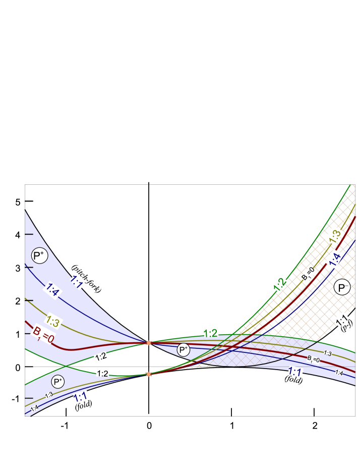
Figure 9: In the $(\tilde{c},\tilde{M})$-plane, three grey and one hatching regions correspond to the existence of elliptic points: $P^{+}$ for the grey regions and $P^{-}$ for the hatching one. Lines corresponding to the main resonances and vanishing the first Birkhoff coefficient for the elliptic point are shown and labelled.

Using this formula we represent in Figure 9 curves $B_{1}(\tilde{c},\tilde{M})=0$, where the elliptic fixed point can be, a priori, not KAM-stable. In this Figure curves related to the strong resonances are presented. For resonances 1:1 and 1:2 the equations of the corresponding curves are given in Section 3.4. The equations of the 1:3 and 1:4 curves are as follows:

$$\tilde{M}=\frac{\tilde{c}^{2}+1}{4}\pm\frac{\sqrt{\tilde{c}^{2}+1}}{2}(1-\tilde{c})\;\;\mbox{for 1:4 resonance}$$

and

$$\tilde{M}=\frac{\tilde{c}^{2}+\tilde{c}+1}{4}\pm\frac{\sqrt{\tilde{c}^{2}+\tilde{c}+1}}{2}(1-\tilde{c})\;\;\mbox{for 1:3 resonance}.$$

This completes the proof.

Acknowledgements. The authors thank D.Turaev and L.Shilnikov for fruitful discussions and remarks. The second, third and fifth authors have been supported partially by the RFBR grants No.07-01-00566, No.07-01-00715 and No.09-01-97016-r-povolj’e. The first and fourth authors have been partially supported by the MICIIN/FEDER grant number MTM2009-06973 and by the Generalitat de Catalunya grant number 2009SGR859. S. Gonchenko thanks Centre de Recerca Matemàtica (Bellaterra) for very nice hospitality in 2008.

References

- [1] Afraimovich V S and Shilnikov L P, 1973, On critical sets of Morse-Smale systems Trans. Moscow Math. Soc. 28, 179-212.
- [2] Bochner S., 1945, Compact groups of differentiable transformations. Ann. Math., second series, vol. 46, 3, 372–381.
- [3] Biragov V.S. “Bifurcations in a two-parameter family of conservative mappings that are close to the Henon map”.- Selecta Math.Sov., 1990, v.9, 273-282. [Originally publ. in “Methods of qualitative theory of differential equations”, Gorky State Univ., 1987, 10-24.]
- [4] Delshams A and Lázaro J T, 2005, Pseudo-normal form near saddle-center or saddle-focus equilibria J. Differential Equations 208(2) 312-343.
- [5] Duarte P, 2000, Persistent homoclinic tangencies for conservative maps near the indentity Ergod. Th. Dyn. Sys. 20 393-438.
- [6] Gavrilov N K and Shilnikov L P, 1972, On three-dimensional dynamical systems close to systems with a structurally unstable homoclinic curve I, Math. USSR Sbornik, 17, 467–485; II, 1973, 19, 139–156.
- [7] Gonchenko S V, 1984, Nontrivial hyperbolic subsets of systems with structurally unstable homoclinic curve. (Russian) Methods of the qualitative theory of differential equations (Russian), 89–102, 200.
- [8] Gonchenko S V and Shilnikov L P, 1990, Invariants of -conjugacy of diffeomorphisms with a structurally unstable homoclinic trajectory Ukrainian Math. J. 42 134-140.
- [9] Gonchenko S V and Shilnikov L P, 1993, Moduli of systems with a structurally unstable homoclinic Poincaré curve Russian Acad. Sci. Izv. Math., 41(3) 417-445.
- [10] Gonchenko S V, Turaev D V and Shilnikov L P, 1993, On models with non-rough Poincaré homoclinic curves Physica D, 62, 1-14.
- [11] Gonchenko S V, Turaev D V and Shilnikov L P, 1993, On the existence of Newhouse regions near systems with non-rough Poincaré homoclinic curve (multidimensional case) Russian Acad. Sci.Dokl.Math., 47.
- [12] Gonchenko S V, Turaev D V and Shilnikov L P, 1997, On Newhouse domains of two-dimensional diffeomorphisms with a structurally unstable heteroclinic cycle Proc. Steklov Inst. Math., 216, 70-118.
- [13] Gonchenko S V, Turaev D V and Shilnikov L P, 2001, Homoclinic tangencies of any order in Newhouse regions J. Math. Sci. 105, 1738-1778.
- [14] Gonchenko S V and Shilnikov L P, 2000, On two-dimensional area-preserving diffeomorphisms with infinitely many elliptic islands J.of Stat.Phys. 101(1/2), 321-356.
- [15] Gonchenko S V and Gonchenko V S, 2000, On Andronov-Hopf bifurcations of two-dimensional diffeomorphisms with homoclinic tangencies WIAS-preprint, Berlin, N.556, 27.
- [16] Gonchenko S V, Stenkin O V and Shilnikov L P, 2002, On Newhouse regions with infinitely many stable and unstable invariant tori Proceedings of the Int.Conf. ”Progress in Nonlinear Science” dedicated to 100th Anniversary of A.A.Andronov, July 2-6 v.1 “Mathematical Problems of Nonlinear Dynamics”, Nizhni Novgorod, 80-102.
- [17] Gonchenko S V and Gonchenko V S, 2004, On bifurcations of birth of closed invariant curves in the case of two-dimensional diffeomorphisms with homoclinic tangencies Proc. Steklov Inst. 244, 80-105.
- [18] Gonchenko S V, Stenkin O V and Shilnikov L P, 2006, On the existence of infinitely many stable and unstable invariant tori for systems from Newhouse regions with heteroclinic tangencies Nonl. Dyn. 2, 3-25.
- [19] Gonchenko V S and Shilnikov L P, 2007, Bifurcations of systems with a homoclinic loop to a saddle-focus with saddle index 1/2. (Russian) Dokl. Akad. Nauk 417 (2007), no. 6, 727–731; translation in Dokl. Math. 76, no. 3, 929–933.
- [20] Gonchenko S V, Shilnikov L P and Turaev D, 2007, Homoclinic tangencies of arbitrarily high orders in conservative and dissipative two-dimensional maps Nonlinearity 20, 241-275.
- [21] Gonchenko S V, Shilnikov L P and Turaev D, 2008, On dynamical properties of multidimensional diffeomorphisms from Newhouse regions Nonlinearity 21(5), 923-972.
- [22] Gonchenko S V, Lamb J and Turaev D V, On typical properties of two-dimensional reversible maps from Newhouse regions to appear.
- [23] Lamb J S W and Stenkin O V 2004, Newhouse regions for reversible systems with infinitely many stable, unstable and elliptic periodic orbits Nonlinearity 17(4), 1217-1244.
- [24] Montgomery D and Zippin L 1955, Topological transformation groups Intersience, New York.
- [25] Moser J and Webster S M 1983 Normal forms for real surfaces in near complex tangents and hyperbolic surface transformations Acta Math. 150, no. 3-4, 255–296.
- [26] Newhouse, S E, 1970, Non-density of Axiom A(a) on , Proc. A.M.S. Symp. Pure Math., 14, pp.191-202.
- [27] Newhouse S, 1974, Diffeomorphisms with infinitely many sinks Topology 13 9-18.
- [28] Newhouse S E, 1979, The abundance of wild hyperbolic sets and non-smooth stable sets for diffeomorphisms Publ. Math. Inst. Hautes Etudes Sci. 50 101-151.
- [29] Palis J and Viana M, 1994, High dimension diffeomorphisms displaying infinitely many sinks Ann. Math. 140 91-136.
- [30] Pikovsky A, Topaj D, 2002, “Reversibility vs. synchronization in oscillator latties”, Physica D, v.170, 118-130.
- [31] Piftankin, G.N. and Treshchev, D V , 2007, Separatrix maps in Hamiltonian systems Uspekhi Mat. Nauk 62:2 3-108 (in Russian), Russian Math. Surveys 62:2 219-322.
- [32] Roberts, J A G , 1997, Some characterisations of low-dimensional dynamical systems with time-reversal symmetry. Math. Model. 8, Control & Chaos.
- [33] Roberts J A G and Quispel G R W , 1992, Chaos and time-reversal symmetry. Order and Chaos in reversible systems. Physics Reports, 216, Numbers 2-3, pages 63–177.
- [34] Rom-Kedar V, 1995, Secondary homoclinic bifurcation theorems Chaos 5, 385–401.
- [35] Romero N, 1995, Persistence of homoclinic tangencies in higher dimensions Ergod. Th. Dyn.Sys. 15 735-757.
- [36] Shilnikov L P, 1967, On a Poincaré-Birkhoff problem Math. USSR Sb. 3 91-102.
- [37] Sevryuk M 1986, Reversible Systems, Lecture Notes in Mathematics, 1211, (Berlin, Heidelberg, New York: Springer-Verlag).
- [38] Shilnikov L P, Shilnikov A L, Turaev D V and Chua L O 1998, Methods of qualitative theory in nonlinear dynamics. Part I (Singapore: World Scientific).
- [39] Siegel CC L and Moser J K, 1995, Lectures on Celestial Mechanics (Berlin, Heidelberg, New York: Springer-Verlag).
- [40] Turaev D, 2003, Polynomial approximations of symplectic dynamics and richness of chaos in non-hyperbolic area-preserving maps Nonlinearity 16, 123-135.