Pre-Turbulent Regimes in Graphene Flows

Abstract

We provide numerical evidence that electronic pre-turbulent phenomena in graphene could be observed, under current experimental conditions, through detectable current fluctuations, echoing the detachment of vortices past localized micron-sized impurities. Vortex generation, due to micron-sized constriction, is also explored with special focus on the effects of relativistic corrections to the normal Navier-Stokes equations. These corrections are found to cause a delay in the stability breakout of the fluid as well as a small shift in the vortex shedding frequency. Finally, a relation between the Strouhal number, a dimensionless measure of the vortex shedding frequency, and the Reynolds number is provided under conditions of interest for future experiments.

Since its recent discovery Novoselov et al. (2005, 2004), graphene has continued to surprise scientists with an amazing series of spectacular properties, such as ultra-high electrical conductivity, ultra-low viscosity to entropy ratio, combination of exceptional structural strength and mechanical flexibility, and optical transparency. Many of these fascinating effects are due to the fact that, consisting of literally a single carbon monolayer, graphene represents the first instance of a truly two-dimensional material (the “ultimate flatland” Geim and MacDonald (2007)). Moreover, due to the special symmetries of the honeycomb lattice, electrons in graphene are shown to behave like an effective Dirac fluid of massless chiral quasi-particles propagating at a Fermi speed of about $v_{F}\sim c/300\sim 10^{6}$ m/s. This configures graphene as a very special, slow-relativistic electronic fluid, where many unexpected quantum-electrodynamic phenomena can take place, Shuryak (2004); Kovtun et al. (2005); Policastro et al. (2001). In particular, the capability of reaching down viscosity to entropy ratios smaller than that of superfluid Helium at the lambda-point, has recently spawned the suggestion that electronic transport in graphene may support pre-turbulent phenomena, Ref. Müller et al. (2009).

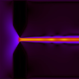
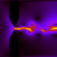
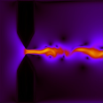
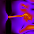
Figure 1: Pre-turbulence at Reynolds number $Re=25$ in graphene is shown: at $379400$ time steps, 1 and 1; and at $603400$ time steps, 1 and 1. For 1 and 1 the term $\partial p/\partial t$ was removed. The color represents the magnitude of the velocity.

In this Letter, we pursue this suggestion in quantitative terms. More precisely, we simulate the relativistic graphene-fluid equations, proposed in Ref. Müller et al. (2009), under conditions of present and prospective experimental realizability. Our main result is that micro-scale impurities, as small as a few microns, are capable of triggering coherent patterns of vorticity in close qualitative and quantitative resemblance with classical two-dimensional turbulence (see e.g. Fig. 1). It is also shown that such vorticity patterns give rise to detectable current fluctuations across the sample, well in excess of flickering noise. As a result, based on our simulations, we conclude that the hydrodynamic picture of graphene as a near-perfect, slow-relativistic fluid, as developed in Ref. Müller et al. (2009), should be liable to experimental verification.

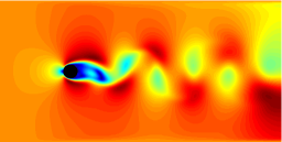
Figure 2: Vortex shedding in graphene at Reynolds number $Re=100$, using a grid of $1024\times 512$ cells. The color scale represents the absolute velocity of the fluid. The picture was taken at $4\times 10^{6}$ time steps.

The equations for the Dirac electron fluid in graphene read as follows Müller et al. (2009): $\partial\rho_{c}/\partial t+\nabla\cdot\left(\rho_{c}\vec{u}\right)=0$, for charge conservation; $\partial\epsilon/\partial t+\nabla\cdot\left[(\epsilon+p)\vec{u}\right]=0$, for energy density conservation and

$$\frac{\epsilon+p}{c^{2}}\left[\frac{\partial\vec{u}}{\partial t}+\left(\vec{u}\cdot\nabla\right)\vec{u}\right]+\nabla p+\frac{\vec{u}}{c^{2}}\frac{\partial p}{\partial t}-\eta\nabla^{2}\vec{u}=0\quad,$$ (1)

for momentum conservation. Here, $c$ is the Fermi speed ($\sim 10^{6}$m/s), $\epsilon$ the energy density, $p$ the pressure, $\rho_{c}$ the charge density, and $\vec{u}$ the velocity. The shear viscosity can be calculated by using Müller et al. (2009)

$$\eta=C_{\eta}\frac{N(k_{B}T)^{2}}{4\hbar c^{2}\alpha^{2}}\quad,$$ (2)

where $C_{\eta}\sim O(1)$ is a numerical coefficient, $T$ is the temperature, $\alpha=e^{2}/\varepsilon\hbar c$ is the effective fine structure constant, $e$ being the electric charge of the electron, $\varepsilon$ the relative dielectric constant, and $N$ the number of species of free massless Dirac particles. Additionally, the entropy density can be calculated according to the Gibbs-Duhem relation $\epsilon+p=Ts$. These equations have been derived under the assumption $|\vec{u}|\ll c$.

The relativistic lattice Boltzmann (RLB), proposed by Mendoza et. al. Mendoza et al. (2010a, b), is hereby adapted to reproduce, in the continuum limit, the equations for the Dirac electron fluid described above. The RLB model Mendoza et al. (2010a) was defined on a three-dimensional lattice with nineteen discrete velocities. Since graphene is $2D$, we have adapted the model to a two-dimensional cell with nine discrete velocities, linking each site to its four nearest-neighbors, four next-to-nearest neighbors (diagonal), plus a rest particle. Two distribution functions, $f_{i}$ and $g_{i}$, are used for the particle number and momentum-energy, respectively. These distribution functions evolve according to the typical Boltzmann equation in single-time relaxation approximation Bhatnagar et al. (1954); Mendoza et al. (2010a), $f_{i}(x+\delta x,t+\delta t)-f_{i}(x,t)=-(f_{i}-f_{i}^{\rm eq})/\tau$ and $g_{i}(x+\delta x,t+\delta t)-g_{i}(x,t)=-(g_{i}-g_{i}^{\rm eq})/\tau$, where $\tau$ is the single relaxation time, and the equilibrium functions $f_{i}^{\rm eq}$ and $g_{i}^{\rm eq}$ are defined in Ref. Mendoza et al. (2010a, b). The shear viscosity, according to this model is $\eta=(\epsilon+p)\left(\tau-\frac{1}{2}\right)c_{l}^{2}\delta t/3c^{2}$, where $c_{l}=\delta x/\delta t$ is the ratio of the lattice spacing to time-step size.

We choose the equation of state $\epsilon=3p$, which depends on temperature in the relativistic regime, as $\epsilon\sim(k_{B}T)^{3}/(c\hbar)^{2}=T^{3}$ (in normalized units $c=\hbar=k_{B}=e=1$) Hartnoll et al. (2007). Thus, the shear viscosity $\eta$ would depend on the third power of the temperature, leading to a different relation than Eq. (2). However, in the Dirac fluid, the relaxation time for the electrons depends on the inverse of the temperature, $\tau_{rel}=(\hbar\alpha)^{2}/k_{B}T$ Fritz et al. (2008), and, therefore, introducing this dependence into the relaxation time $\tau$ of the numerical model, we obtain the correct function for the viscosity. In numerical units ($\delta x=\delta t=c=1$), we set the relaxation time to $\tau=\tau_{0}T_{0}/T+1/2$, where $T_{0}$ is the initial temperature and $\tau_{0}$ the initial relaxation time.

The hydrodynamics equations are similar to the non-relativistic Navier-Stokes equations with the exception of the compressibility term $\sim\partial p/\partial t$. This term is most likely negligible at low frequencies, but it may become relevant at higher ones. The Reynolds number $Re$, measuring the strength of inertial versus dissipative terms Müller et al. (2009), is given by $Re=(sT/c^{2})(LU_{typ}/\eta)$, where $L$ and $U_{typ}$ are the characteristic length and flow velocity of the system, respectively. In lattice units, it reads as

$$Re=\frac{3LU_{typ}}{c^{2}\delta t\left(\tau-\frac{1}{2}\right)}\quad.$$ (3)

According to classical turbulence theory, vortex shedding in graphene is expected for Reynolds numbers well above one, typically $Re\sim 10\div 100$. To detect signatures of pre-turbulent behavior in graphene experiments, one can measure the fluctuations of the electric current through the graphene sample. The current density is defined by $\vec{j}=\rho_{c}\vec{u}$, and the total electric current is calculated integrating the current density along the transverse ($y$) coordinate. The characteristic fluctuation frequency can then be related to the vortex shedding frequency. Macroscopic speeds $u\sim 10^{5}$ m/s could be achieved by the electrons in grapheneMeric et al. (2008). The Reynolds number rewrites as: $Re=U_{typ}LT/c^{2}(\eta/s)$. According to Ref. Müller et al. (2009), $\eta/s$ takes values around $0.2\hbar/k_{B}$, at temperature of $300$K, so that we can write $Re=U_{typ}L/\nu_{eff}$, $\nu_{eff}=c^{2}\eta/Ts\sim 0.005$ m²/s being the effective kinematic viscosity. Therefore, a sample of size $L=5\mu$m, within reach of current technology, would yield $Re\sim 100$, sufficiently high to trigger pre-turbulent phenomena, such as vortex shedding. To test the idea on quantitative grounds, we implement a simulation on a grid with $1024\times 512$ cells. The following initial values (numerical units) were used: $\epsilon=0.75$, $\rho_{c}=1.0$, $\vec{u}=(u_{x},0)=(0.002,0)$, and the Fermi speed $c=c_{l}=1.0$. The initial value of the relaxation time was chosen $\tau_{0}=0.003$ such that the initial shear viscosity $\eta=\frac{1}{3}\left(\tau-\frac{1}{2}\right)=10^{-3}$.

A circular obstacle, with diameter $D=50$, is introduced at $(256,256)$, modeling a $5$ micron diameter impurity in the graphene sample (Fig. 2). With this configuration, and setting $L=D$ in Eq. 3, the Reynolds number for this system is $Re\sim 100$. We choose periodic boundary conditions at top and bottom, and demand that the distribution functions of the boundary cells are always equal to the equilibrium distribution functions evaluated with the initial conditions. Free boundary conditions are imposed at the outlet. At the left border, we set inlet conditions, where the missing information of the distribution functions is filled by the equilibrium distribution function corresponding to the initial conditions Succi (2001). We define $\delta t=0.05\text{ps}$.

The drag $F_{Dx}$ and lift $F_{Dy}$ forces acting on the obstacle are measured, the vortex shedding frequency being computed in terms of fluctuations of the lift forces. We compare the frequency of the electric current fluctuations with the frequency of the drag force, which, in general, is twice the vortex shedding frequency (see Fig. 3). To relate these to the vortex shedding, we use a fast-Fourier transform (FFT). As is well visible from Fig. 3, the current fluctuations contribute about one part per thousand of the base signal, and, consequently, they should be liable to experimental detection.

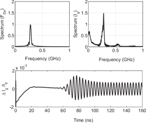
Figure 3: FFT of the electric current fluctuations $\Delta I_{g}$, in the graphene sample (top right), due to the vortex shedding as a function of time. Also, it is shown the FFT of the drag force acting on the obstacle (top left). This result refers to $Re=100$. At the bottom, the fluctuations in the electric current $I_{g}$ are shown as a function of time.

In future applications, involving larger graphene samples, higher Reynolds numbers will be attained. Consequently, it becomes of interest to assess the role of the relativistic corrections to the classical Navier-Stokes equations.

Comparing the dynamics of the relativistic and non-relativistic fluids, two basic differences emerge: the relativistic correction term $\sim\partial p/\partial t$; and the viscosity dependence with the temperature, Eq. (2). In order to assess whether these terms play an important role, we implement three simulations on a grid of size $2048\times 1024$ cells. In the first simulation, we model the full relativistic equations; in the second one, the relativistic effect $\sim\partial p/\partial t$ is removed; and in the third one, the viscosity is forced to be a constant. The same initial configuration, as before, is used with the exception of: $\vec{u}=(u_{x},0)=(0.03,0)$ and $D=100$ (in this case, modeling an impurity of diameter $150\mu$m). The impurity is now centered at $(512,512)$. With this configuration, Eq. 3 gives $Re\sim 3000$. The simulations run up to $10^{6}$ time steps (with $\delta t=1.5\text{ps}$).

From Fig. 4, we find that, in the case of constant viscosity, the frequency is a bit higher than the one corresponding to the full relativistic case. On other hand, if the term $\sim\partial p/\partial t$ is removed from the equations, the frequency decreases. We conclude that, in order to compare to high precision measurements of the vortex shedding frequencies, these terms cannot be ignored.

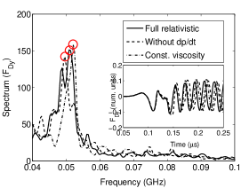
Figure 4: Frequencies of the vortex shedding at Reynolds number $Re=3000$, using a grid of $2048\times 1024$ cells, are shown. These are calculated for three different cases: the full relativistic, relativistic without the term $\partial p/\partial t$, and relativistic with constant viscosity.

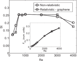
Figure 5: Strouhal number $St$ as a function of the Reynolds number $Re$ for both non-relativistic and relativistic fluids. In the inset, the mean value of the $x$-component of the drag force as a function of the Reynolds number is shown. The error bar is of the size of the symbol.

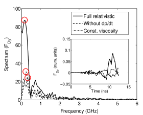
Figure 6: The same case of Fig. 4, but in the case of the constriction at Reynolds number $Re=25$, using a grid with $1024\times 1024$ cells.

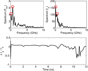
Figure 7: The same case as Fig. 3 for the constricted flow at $Re=25$.

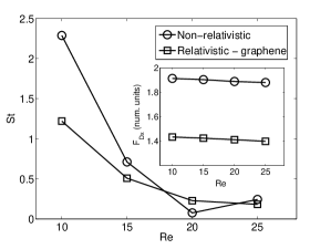
Figure 8: The same as Fig. 5 for the case of the constriction.

To study the frequency of the vortex shedding, we vary the initial velocity in order to obtain different Reynolds numbers. The Strouhal number $St$ is defined as the dimensionless frequency of the vortex shedding and can be calculated as $St=f_{s}L/U_{typ}$, where $f_{s}$ is the frequency of the vortex shedding. Fig. 5 shows that the relation between $St$ and $Re$ is very similar for the relativistic and non-relativistic fluids, with a fast growth of $St$ in the range $200<Re<1000$, followed by a flat-top at $St\sim 0.25$ Williamson (1989, 1988); Ponta and Aref (2004) for $Re>1000$. From the Strouhal number, we can obtain the frequencies of the vortex shedding, as $f_{s}=0.2U_{typ}/L$. The frequency of the drag force is twice that of vortex shedding, namely $f_{Ds}=0.4U_{typ}/L$. As a result, once the Reynolds number is known, one can compute the frequency of the drag force, the Strouhal number, and then compare with the FFT of the electric current measurement in the sample. The mean value of the drag force $\overline{F}_{Dx}$, reported in the inset of Fig. 5 as a function of the Reynolds number, shows a monotonic dependence in the range of $Re$ explored here.

Another kind of set-up to detect pre-turbulence in graphene experiments, with the possibility of being implemented nowadays, consists of building a constriction, where the Dirac fluid can develop vorticity patterns as it crosses through. Fig. 1 shows the vorticity at $Re=25$, where the characteristic length $L=50$ cells has been chosen as the distance between the tips. In this case, the initial velocity is taken $\vec{u}=(u_{x},0)=(0.0005,0)$, in lattice units, and the simulation is performed using a grid of $1024\times 1024$ cells. We simulate two systems, one with the full relativistic equations and the other one by just removing the relativistic term $\partial p/\partial t$. From the simulations (see Fig. 1), we conclude that the relativistic contribution affects the time to the onset of instability, and, from Fig. 6, we can appreciate that, as for the circular impurity, the frequency of the vortices presents a shift due to the relativistic corrections. However, both constant viscosity and removal of the relativistic correction, contribute to an increase of the frequency of the fluctuations. Fig. 7 shows how such fluctuations can be measured, and the characteristic frequencies (see red circles in Fig. 7) related with the drag force acting on the constriction. Note that, in order to achieve $Re=25$, at a speed of $0.1c$, the distance between tips is about $1.25\mu$m.

As for the case of the circular impurity, we can find the characteristic relation between the Strouhal number and the Reynolds number for this geometrical set-up (see Fig. 8). From the inset of Fig. 8, we observe that the drag force decreases slightly, as the Reynolds number is increased, and exhibits a noticeable difference between the non-relativistic and relativistic cases.

Summarizing, we have shown that, in the range of $Re\sim 10^{2}$, vorticity patterns can be indirectly observed by measuring the electric current fluctuations in the graphene sample. However, using a different geometry, like a constriction, signatures of pre-turbulence can be detected already at Reynolds numbers as small as $Re\sim 25$. We have also compared the effects of relativistic corrections, such as dynamic compressibility and the dependency of the viscosity on the temperature, on the dynamics of the system. In these cases, the temperature dependency of the viscosity and the term $\partial p/\partial t$ produce a shift in the frequencies of the vortex shedding and, therefore, in the electric current fluctuations. Additionally, the relativistic correction term, $\sim\partial p/\partial t$, is found to delay the instability process in the case of the constricted flow. For future applications, most likely accessing higher Reynolds numbers, the frequency of the vortex shedding can be calculated using the Strouhal number, thereby permitting to distinguish current fluctuations induced by pre-turbulent phenomena from those resulting from other physical effects.

We thank K. Ensslin for enlightening discussions.

References

- Novoselov et al. (2005) K. Novoselov, A. Geim, S. Morozov, D. Jiang, M. Katsnelson, I. Grigorieva, and S. Dubonos, Nature Letters 438, 197 (2005).
- Novoselov et al. (2004) K. S. Novoselov, A. K. Geim, S. V. Morozov, D. Jiang, Y. Zhang, S. V. Dubonos, I. V. Grigorieva, and A. A. Firsov, Science 306, 666 (2004).
- Geim and MacDonald (2007) A. K. Geim and A. H. MacDonald, Phys. Today p. 35 (2007).
- Shuryak (2004) E. Shuryak, Progress in Particle and Nuclear Physics 53, 273 (2004), ISSN 0146-6410, heavy Ion Reaction from Nuclear to Quark Matter.
- Kovtun et al. (2005) P. K. Kovtun, D. T. Son, and A. O. Starinets, Phys. Rev. Lett. 94, 111601 (2005).
- Policastro et al. (2001) G. Policastro, D. T. Son, and A. O. Starinets, Phys. Rev. Lett. 87, 081601 (2001).
- Müller et al. (2009) M. Müller, J. Schmalian, and L. Fritz, Phys. Rev. Lett. 103, 025301 (2009).
- Mendoza et al. (2010a) M. Mendoza, B. M. Boghosian, H. J. Herrmann, and S. Succi, Phys. Rev. Lett. 105, 014502 (2010a).
- Mendoza et al. (2010b) M. Mendoza, B. M. Boghosian, H. J. Herrmann, and S. Succi, Phys. Rev. D 82, 105008 (2010b).
- Bhatnagar et al. (1954) P. Bhatnagar, E. P. Gross, , and M. Krook, Phys. Rev. 94, 511 (1954).
- Hartnoll et al. (2007) S. A. Hartnoll, P. K. Kovtun, M. Müller, and S. Sachdev, Phys. Rev. B 76, 144502 (2007).
- Fritz et al. (2008) L. Fritz, J. Schmalian, M. Müller, and S. Sachdev, Phys. Rev. B 78, 085416 (2008).
- Meric et al. (2008) I. Meric, M. Y. Han, A. F. Young, B. Ozyilmaz, P. Kim, and K. L. Shepard, Nature Nanotech. 3, 654 (2008).
- Succi (2001) S. Succi, The Lattice Boltzmann Equation for Fluid Dynamics and Beyond (Oxford University Press, USA, 2001), ISBN 0198503989.
- Williamson (1989) C. H. K. Williamson, Journal of Fluid Mechanics 206, 579 (1989).
- Williamson (1988) C. H. K. Williamson, Physics of Fluids 31, 3165 (1988).
- Ponta and Aref (2004) F. L. Ponta and H. Aref, Phys. Rev. Lett. 93, 084501 (2004).