The cosmic spin of the most massive black holes

Abstract

Under the assumption that jets in active galactic nuclei are powered by accretion and the spin of the central supermassive black hole, we are able to reproduce the radio luminosity functions of high- and low-excitation galaxies. High-excitation galaxies are explained as high-accretion rate but very low spin objects, while low-excitation galaxies have low accretion rates and bimodal spin distributions, with approximately half of the population having maximal spins. At higher redshifts ($z\sim$1), the prevalence of high accretion rate objects means the typical spin was lower, while in the present day Universe is dominated by low accretion rate objects, with bimodal spin distributions.

1 Introduction

Active galactic nuclei (AGN) are galaxies with signs of non-stellar activity in their centres, believed to be powered by supermassive black holes (SMBHs). AGN produce jets which are observable at radio frequencies. For a given accretion rate, AGN can produce jets which vary in radio luminosity by several orders of magnitude. Conversely, for a given radio luminosity, some AGN are found to have very high accretion rate, while others are found to have very low ones.

The hidden variable behind this ‘radio loudness’ of AGN has often been connected with the spin of the SMBH, $\hat{a}$, and this is known as the ‘spin paradigm’ (e.g. Wilson & Colbert 1995; Sikora et al. 2007). Indeed theory and simulations suggest that spinning SMBHs should be able to power considerable jets (e.g. Blandford & Znajek, 1977, Hawley & Krolik 2006, Tchekhovskoy et al. 2010), and indeed observations of the most powerful radio galaxies require an extremely efficient mechanism for the production of jets (e.g. Punsly 2007, Fernandes et al. 2011).

Recently, Fender et al. (2010) have noted a lack of correlation between the reported measurements of jet powers and black hole spin for galactic black holes in X-ray binaries. As we discuss in detail in Martínez-Sansigre & Rawlings (2011, hereafter MSR11), the uncertainties in both measurements are very large, so that the lack of observed correlation does not provide robust evidence against the spin paradigm (see Section 7.2 of MSR11 for a detailed discussion).

In this work we infer the cosmic distribution of SMBHs spins under the assumption that spin is the major variable explaining the huge variations in jet power. Indeed models and simulations of spinning black holes can provide enough variation in jet power to explain most of the variation in radio loudness of AGN (see Section 3 of MSR11).

Under this assumption, we derive the spin distributions for SMBHs with high and low accretion rates, and infer the cosmic spin history. Throughout our work we concentrate on the most massive black holes, with $m_{\bullet}$$\geq 10^{8}$ M_⊙. This is achieved by working only with radio luminosity densities $\geq 10^{23}$ W Hz^-1 sr^-1, where all the AGN black hole masses are known to be $\geq 10^{8}$ M_⊙  (McLure et al. 2004, Smolčić et al. 2009).

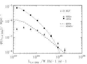
Figure 1: (Left panel): Best-fit to the local radio LF of the ADAF and QSO components. The black circles represent the observed radio LF of LEGs, the empty triangles represent the HEGs. (Right panel): Spin distribution for all SMBHs in the locl Universe, obtained by combining the individual spin distributions of ADAFs and QSOs, weighted by their space densities (see Equation 8).

1.1 Assumptions

The bolometric power available for radiation is given by:

$$L_{\rm bol}=\epsilon(\hat{a})\dot{m}_{\bullet}c^{2}$$ (1)

where $L_{\rm bol}$ is the bolometric luminosity due to radiation, $\dot{m}_{\bullet}$ is the rate of accretion of mass onto the SMBH, and the term $\epsilon(\hat{a})$ is the radiative efficiency (Novikov & Thorne 1973).

We assume that the power available for the production of jets can be described as a function of accretion rate and spin only:

$$Q_{\rm jet}=\eta(\hat{a})\dot{m}_{\bullet}c^{2}$$ (2)

where $Q_{\rm jet}$ is the jet power and $\eta(\hat{a})$ is the jet efficiency. This is a simplification, which ignores the dependence of the jet power on the geometry of the accretion flow. For more details see MSR11. In these proceedings we only show the results using one particular set of jet efficiencies, from the 3D general relativistic magnetohydrodynamic simulations of Hawley & Krolik (2006). However, in MSR11 we show the results for a set of six different efficiencies, and find the results to be robust.

Finally, to convert from jet power to observed ratio luminosity at 151 MHz, we follow the conversion derived by Willott et al. (1999):

$$\left({Q_{\rm jet}\over{\rm W}}\right)=3\times 10^{38}f^{3\over 2}\left({L_{\nu 151}\over 10^{28}~{}{\rm WHz^{-1}sr^{-1}}}\right)^{6\over 7}$$ (3)

and assume $f=$20 (see MSR11 for more details, and also Cavagnolo et al. 2010). The term $f$ is one of the dominant sources of uncertainty in our work. We convert from 151 MHz to 1.4 GHz assuming a power law with index -0.75.

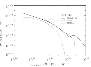
Figure 2: (Left panel): Comparison of the $z=$1 predicted and observed radio LFs. The solid line represents the observed luminosity function (Willott et al. 2001, Smolčić et al. 2009). The dashed line is the predicted QSO contribution, the dotted line is the ADAF contribution. (Right panel): The corresponding spin distribution of SMBHs at $z=$1.

2 Modelling the local radio luminosity function

Best et al. (in prep.) have classified the radio sources of the local radio luminosity function (LF), according to their optical spectra. Sources have been classified into high-excitation and low-excitation galaxies (HEGs and LEGs, respectively), and individual radio LFs have been derived.

We model these two populations independently. For the HEGs, we assume that these represent SMBHs accreting at a significant fraction of their Eddington limiting (‘QSOs’). The X-ray LF provides us with the space density of SMBHs with high accretion rates (Silverman et al. 2008). The bolometric luminosity, $L_{\rm bol}$, can be estimated from the X-ray luminosity $L_{\rm X}$, via a bolometric correction, $C_{\rm X}$, so that $L_{\rm bol}$$=$$C_{\rm X}L_{\rm X}$. Using equations 1 and 2, the jet power can be estimated using:

$$Q_{\rm jet}={\eta(\hat{a})C_{\rm X}L_{\rm X}\over\epsilon(\hat{a})}.$$ (4)

Hence, given a spin we can infer the jet power from the X-ray luminosity. We model the space density of HEGS with a given radio luminosity as:

$$\phi_{\rm QSO}(L_{\nu})={{\rm d}Q_{\rm jet}\over{\rm d}L_{\nu}}\int P_{\rm QSO}(\hat{a})\phi(L_{\rm X}){{\rm d}L_{\rm X}\over{\rm d}\dot{m}}{\rm d}\hat{a}.$$ (5)

The term $\phi_{\rm QSO}(L_{\nu})$ is the modelled radio LF of QSOs, which we use to explain the HEGs, $\phi(L_{\rm X})$ is the X-ray LF, and $P_{\rm QSO}(\hat{a})$ is the distribution of spins for the QSOs. ${\rm d}Q_{\rm jet}/{\rm d}L_{\nu}$ is computed from Equation 3. For details of the derivation of Equation 5 we refer the reader to Section 4.1 of MSR11. The X-ray LF is integrated above X-ray luminosities that can only be reached by SMBHs with $m_{\bullet}$$\mathrel{\hbox{\hbox to0.0pt{\hbox{\lower 2.0pt\hbox{$\sim$}}\hss}\raise 2.0pt\hbox{$>$}}}10^{8}$ M_⊙. We note that we include a correction factor to account for the fraction of QSOs that are optically-thick to Compton scattering and hence missed by the hard X-ray surveys (e.g. Martínez-Sansigre et al. 2007).

For the LEGs, we model these as low-Eddington rate objects (‘ADAFs’). We do not have direct access to an ADAF LF. However, the local mass function of SMBHs is known (e.g. Graham et al. 2007), so we can use it to model the space density of ADAFs. Given a black hole mass, $m_{\bullet}$, the Eddington limiting accretion rate is given by $\dot{m}_{\rm E}c^{2}=L_{\rm E}m_{\bullet}/\epsilon$, where $L_{\rm E}$ is the Eddington limiting luminosity, 1.3$\times 10^{31}$ W M_⊙^-1. Hence, given a black hole mass and an Eddington rate, $\lambda\equiv\dot{m}/\dot{m}_{\rm E}$, we can estimate the jet power:

$$Q_{\rm jet}={\eta(\hat{a})\lambda\dot{m}_{\rm E}}.$$ (6)

Given the space density of SMBHs with a mass $m_{\bullet}$, $\phi(m_{\bullet})$, the space density of radio sources powered by ADAFs, $\phi_{\rm ADAF}(L_{\nu})$, is given by:

$$\phi_{\rm ADAF}(L_{\nu})=$$

$${{\rm d}Q_{\rm jet}\over{\rm d}L_{\nu}}\int P_{\rm ADAF}(\hat{a})\int P(\lambda)\phi(m_{\bullet}){{\rm d}\lambda\over{\rm d}\dot{m}^{\prime}}{\rm d}m_{\bullet}{\rm d}\hat{a},$$ (7)

where $P_{\rm ADAF}(\hat{a})$ is the spin distribution of ADAFs and $P(\lambda)$ is our prior for the distribution of Eddington ratios (again see MSR11 for more details). Given our ignorance of the distribution of Eddington ratios, we assign a flat prior in log space, with uniform probability density in the range $-8\leq{\rm log}_{10}\lambda\leq-2$.

The only free parameters are the terms describing the spin distributions $P_{\rm QSO}(\hat{a})$ and $P_{\rm ADAF}(\hat{a})$. We use the data to constrain the best fitting parameters for three different spin distributions: a power law, a single gaussian and a double gaussian. The bayesian odds ratio is used to choose between models.

Figure 1 (left panel) shows the observed radio LFs for HEGs and LEGs, and overlayed are the best-fitting $\phi_{\rm QSO}(L_{\nu})$ and $\phi_{\rm ADAF}(L_{\nu})$. The best fitting distribution for the QSOs is a single gaussian centred around $\hat{a}$$=$0.00, for the ADAFs it is a double gaussian, centred at $\hat{a}$$=$0.06 and 0.99, and with the high-spin gaussian having an amplitude of 0.79 compared to the low-spin gaussian.

Hence, we find that the high-accretion rate SMBHs (QSOs/HEGs) have typically low spins, while amongst the low-accretion rate SMBHs (ADAFs/LEGs) there is a high fraction of objects with high spins.

The typical spin distribution for all SMBHs at $z$$=$0 can be estimated from the weighted mean:

$$P_{\rm SMBH}(\hat{a})=$$

$${\sum\phi_{\rm QSO}(L_{\nu})P_{\rm QSO}(\hat{a})+\sum\phi_{\rm ADAF}(L_{\nu})P_{\rm ADAF}(\hat{a})\over\sum\phi_{\rm QSO}(L_{\nu})+\sum\phi_{\rm ADAF}(L_{\nu})}$$ (8)

The right panel of Figure 1 shows $P_{\rm SMBH}(\hat{a})$ in the local Universe.

3 Predicting the $z=$1 radio luminosity function

We now test whether our modelling can reproduce the radio LF at $z=$1. From the observed X-ray LF, we can model the evolution of the QSOs.

No such information is available for the ADAFs, however. Given that the bulk of the growth of the most massive black holes, with $m_{\bullet}$$\geq 10^{8}$ M_⊙, ocurred in the range $1\mathrel{\hbox{\hbox to0.0pt{\hbox{\lower 2.0pt\hbox{$\sim$}}\hss}\raise 2.0pt\hbox{$>$}}}z\mathrel{\hbox{\hbox to0.0pt{\hbox{\lower 2.0pt\hbox{$\sim$}}\hss}\raise 2.0pt\hbox{$>$}}}3$, make the assumption that there has been negligible evolution in the mass function of SMBHs. This assumption is supported by the weak evolution observed amongst radio sources of moderate luminosity (e.g. Smolčić et al. 2009). Hence, at $z=$1 we use the local SMBH mass function, with the same distribution of Eddington ratios.

Figure 2 (left panel) shows the resulting radio LF for QSOs (dashed) and ADAFs (dotted), compared to the observed radio LF (solid line). Without any more free parameters, only the assumption of no evolution for the ADAFs, we are able to approximately reproduce the $z=$1 radio LF over six decades of radio luminosity.

Figure 3: (Left panel): Evolution of the mean spin inferred from our spin distributions for all SMBHs as a function of $z$. The solid line is the mean, the dashed-dotted line shows the standard deviation (note the -1$\sigma$ goes along the x axis). (Right panel): Evolution of the mean spin from the cosmological simulation of Fanidakis et al. (2011), for $m_{\bullet}$$\geq 10^{8}$ M_⊙.

4 The evolution in cosmic spin of SMBHs

Applying Equation 8 to $z=$1, we obtain the spin distribution for all SMBHs at $z=$1, which is shown in the right panel of Figure 2. We see that at high redshift, the fraction of SMBHs with high spin is lower than at low redshift.

It is expected that at $z\geq 1$ the mass function of SMBHs will begin to decrease significantly in space density. This suggests that the space density of ADAFs will also decrease, so that we expect the spin distributions at higher redshifts to be even more dominated by the $\hat{a}$$\sim$0 term.

The evolution of the spin of SMBHs can therefore be understood as a gradual switch between two populations. At high redshift, a high-accretion rate but low spin population dominates (the QSOs). This population decreases strongly in space density as $z$ decreases, revealing a second population of low-accretion sources, which have a bimodal spin distribution (the ADAFs).

This evolution is best described by the spin distributions, as illustrated by the right-hand panels of Figures 1 and 2. However, for completeness we also show the evolution of the mean spin (the expectation value) as a function of redshift, in Figure 3 (left panel). This shows a modest evolution from $\langle\hat{a}(z)\rangle$$\sim$0.2 at $z\sim 1$, to $\langle\hat{a}(z)\rangle$$\sim$0.35 in the local Universe, and when extrapolated to higher redshifts, predicts a mean radiative efficiency $\sim$0.065, in excellent agreement with observational constraints (e.g. Martínez-Sansigre & Taylor 2009).

5 Discussion

We have found that the population dominanting the radio luminosity function switches from high-accretion rate objects with low spins at high redshift, to low-accretion rate objects with a bimodal distribution of spins, with approximately half the population having maximal spin.

This can be explained by the effects on the spin of SMBHs by the two mechanisms by which these grow: accretion and mergers. Continous accretion along one plane would lead to SMBHs having essentially maximal spin. However, it has been recently suggested that SMBHs do not accrete in this way, but are rather subject to ’chaotic accretion’, where matter falls in from different directions. Approximately half of the matter has angular momentum in the opposite direction to the SMBH, and the final spin is therefore, on average, close to 0. Hence accretion provides a mechanism for spinning SMBHs down (King et al. 2008).

Major mergers of SMBHs, on the other hand, are likely to increase the final spin (e.g. Rezzolla et al. 2008). When two black holes of similar mass merge, the angular momentum of the final orbit will be significant compared to the final mass, so that the spin of the coalesced black hole will be large.

The evolution of the spin distributions inferred in our work is in good agreement with a picture where at high redshift the spins are typically low due to accretion. Major mergers will occur both at high and low redshift, but at high redshift there is a larger supply of cold gas available (Obreschkow & Rawlings 2009), so that accretion will spin the SMBHs back down.

At low redshift, the cold gas is running out, so after the mergers the breaking mechanism is no longer present. If a large fraction of the SMBHs have undergone a recent major merger, then a large fraction of the SMBHs will retain a high spin.

A detailed cosmological simulation of the growth of SMBHs was performed by Fanidakis et al. (2011), which included the effects of black hole mergers as well as chaotic accretion. The left panel of Figure 3 shows the mean spin from their simulation, as a function of redshift. The simulation shows an almost identical evolution to that inferred from our work, and a very similar, large variance.