Error Performance of Multidimensional Lattice Constellations - Part I: A Parallelotope Geometry Based Approach for the AWGN Channel

Abstract

Multidimensional lattice constellations which present signal space diversity (SSD) have been extensively studied for single-antenna transmission over fading channels, with focus on their optimal design for achieving high diversity gain. In this two-part series of papers we present a novel combinatorial geometrical approach based on parallelotope geometry, for the performance evaluation of multidimensional finite lattice constellations with arbitrary structure, dimension and rank. In Part I, we present an analytical expression for the exact symbol error probability (SEP) of multidimensional signal sets, and two novel closed-form bounds, named Multiple Sphere Lower Bound (MLSB) and Multiple Sphere Upper Bound (MSUB). Part II extends the analysis to the transmission over fading channels, where multidimensional signal sets are commonly used to combat fading degradation. Numerical and simulation results show that the proposed geometrical approach leads to accurate and tight expressions, which can be efficiently used for the performance evaluation and the design of multidimensional lattice constellations, both in Additive White Gaussian Noise (AWGN) and fading channels.

I Introduction

The employment of Signal Space Diversity (SSD)-a method which has been introduced in [1] to compensate for the degradation caused by fading channels-to multidimensional lattice constellations, has attracted the interest of both academia and industry. By performing component interleaving, new multidimensional signal sets can be designed, which can achieve diversity gain without any additional requirements for power, bandwidth or multiple antennas, but only through rotation of the multidimensional constellation. Such signal sets that have the potential to achieve full diversity, have been presented in the pioneer works [1, 2, 3, 4, 5] and are carved from rotated multidimensional lattices, which meet the criterion of the maximization of the minimum product distance. Multidimensional constellations are also used in Multiple Input-Multiple Output (MIMO) systems [6, 7], cooperative communication systems [8] and various coded schemes [9, 10, 11], while SSD has been included in the Second Generation Digital Terrestrial Television Broadcasting System (DVB-T2) standard [12].

I-A Motivation

Although the evaluation of the performance of such rotated multidimensional signal sets can be an important tool in their design, the study of the symbol error probability (SEP) is in general a hard problem, both in Additive White Gaussian Noise (AWGN) and in fading channels. This is mainly due to the difficulty in the analytical computation of the Voronoi cells of multidimensional constellations[13], and the fact that fading acts independently upon each of the coordinates of the signal, thus making stochastic not just the power but also the structure of the lattice.

Various methods have been presented in order to evaluate the performance of such signal sets, based on either approximations [14], union bounds [15], or bounds on the maximization of the minimum product distance concerning algebraic constructions, such as in [16]. Only recently, some exact expressions for the SEP of two-dimensional constellations have been presented in [17] for Ricean fading channels; however, the extension of such an analysis to multiple dimensions seems to be complicated.

The sphere lower bound (SLB), which dates back to Shannon’s work [18], has been proposed as an efficient tool for evaluating the performance of multidimensional constellations. By approximating the decision regions of infinite lattice constellations - that is multidimensional constellations with infinite number of points - with a sphere of the same volume, a tight lower bound on their error performance can be obtained. This bound in the presence of AWGN has been investigated in [13, 19], while in a similar manner, a sphere upper bound (SUB) based on the packing radius of the lattice, has been presented in [13]. Although both of these sphere bounds have been investigated in AWGN, their performance in the presence of fading has not been thoroughly explored so far. In [20], the performance of SLB in Rayleigh channels was approximated via a geometrical approach, while in [21] it was evaluated for Nakagami-m block fading channels through numerical methods. However, it was clearly demonstrated that, although it is a lower bound for infinite lattice constellations, it is not generally a lower bound for finite lattice constellations. Regarding the SUB, to the best of the authors knowledge, its performance in the presence of fading has not been previously investigated. Moreover, while the SUB is an upper bound also for finite lattice constellations, it is rather loose.

I-B Contribution

In this two-part paper, we provide an analytical framework for the SEP evaluation of multidimensional finite lattice constellations. Our analysis can be efficiently applied to multidimensional signal sets, with arbitrary lattice structure, dimension and rank, taking into account their common geometrical property: the constellations form parallelotopes in the multidimensional signal space.

More specifically, in Part I we introduce a combinatorial approach for the evaluation of the error performance of these signal sets, based on the parallelotope geometry. Following this approach, we derive an analytical expression for the exact SEP of multidimensional finite lattice constellations, which is then lower- and upper-bounded by two novel closed-form expressions, called Multiple Sphere Lower Bound (MSLB) and Multiple Sphere Upper Bound (MSUB) respectively. The MSLB is a new lower bound which - in contrast with the SLB - takes into account the boundary effects of a finite constellation. Similarly the MSUB, also taking into account the boundary effects, is a tighter upper bound in comparison with the SUB.

These expressions can be easily extended to multidimensional signal sets distorted by fading. The error performance evaluation in fading channels is investigated in Part II[22]. Analytical expressions, which bound the frame error probability in block fading channels, are derived for the MSLB and the MSUB, while closed-form expressions are further presented for the SLB and SUB in block fading. This set of expressions proves to be a powerful tool for the error performance analysis of multidimensional constellations, which employ SSD in order to combat the fading degradation.

The remainder of the Part I is organized as follows. In Section II, the structure and properties of infinite and finite lattice constellations are described and the geometry of multidimensional parallelotopes is discussed. Section III presents the system model, while an expression for the exact performance of finite lattice constellations in the AWGN channel is derived and the the MSLB and MSUB are introduced. The simulation results of various constellations and the analytical bounds are discussed in Section IV.

II Lattices and Parallelotope Geometry

II-A Infinite Lattice Constellations

An infinite lattice constellation lying in an $N$-dimensional space consists of all the points of a lattice denoted by $\Lambda.$ A lattice $\Lambda$ is called a full rank lattice when all of its points can be expressed in terms of a set of $N$ independent vectors $\mathbf{v_{i}}$, $i=1,\ldots,N$, called basis vectors. In full rank lattices, every lattice point is given by

$$\Lambda=\mathbf{M}\mathbf{z},\,\,\,\,\,\,\,\,\mathbf{z}\in\mathbb{Z}^{N},$$ (1)

where $\mathbf{M}\in\mathbb{R}^{N\times N}$ is the generator matrix and $\mathbf{z}\in\mathbb{Z}^{N}$ is a vector whose elements are integers. Each different vector $\mathbf{z}$ corresponds to a different point on the lattice $\Lambda$.

The columns of the generator matrix $\mathbf{M}$ are the basis vectors $\mathbf{v_{i}}$, that is

$$\begin{array}[]{ccc}\mathbf{M}=[\mathbf{v_{1}}\,\,\mathbf{v_{2}}\,\,\ldots\,\,\mathbf{v_{N}}],&\mathbf{v_{i}}=[v_{i1}\,\,v_{i2}\,\,\ldots\,\,v_{iN}]^{T},&i=1,2,\ldots,N.\end{array}$$ (2)

The parallelotope consisting of the points

$$\theta_{1}\mathbf{v_{1}}+\theta_{2}\mathbf{v_{2}}+\ldots+\theta_{N}\mathbf{v_{N}},\,\,\theta_{i}=\{0,1\},$$ (3)

is called the fundamental parallelotope of the lattice which tessellates Euclidean space. The volume of the fundamental parallelotope is $\mathrm{vol}(\Lambda)=|\mathrm{det}(\mathbf{M})|$.

We call the Voronoi cell, $\mathcal{V}_{\Lambda}$, of a lattice point $s_{i}$, the region $\mathbf{R}$ for which holds that [13]

$$\mathcal{V}_{\Lambda}=\{x\in\mathbf{R}:\|x-s_{i}\|\leq\|x-s_{j}\|\text{ for all }i\neq j\}.$$ (4)

In an infinite lattice constellation, the Voronoi cell also tessellates Euclidean space, and thus, it is also $\mathrm{vol}(\mathcal{V}_{\Lambda})=|\mathrm{det}(\mathbf{M})|$. Next, this volume is normalized to be $|\mathrm{det}(\mathbf{M})|=1$, as in [21, 23].

II-B Finite Lattice Constellations

We consider finite lattice constellations, denoted by $\Lambda^{\prime}$, which are carved from an infinite $N$-dimensional lattice constellation $\Lambda$ and they can be defined with respect to the generator matrix $\mathbf{M}$ of the lattice $\Lambda$, from which $\Lambda^{\prime}$ is carved. Each of these constellations have $K$ points along the direction of each basis vector, thus having a parallelotope as a shaping region, formed by the vector basis of the infinite lattice constellation $\Lambda$. These constellations will be denoted by a $K$-Pulse Amplitude Modulation ($K$-PAM), since we assume that they are constructed by a PAM signal set along each basis vector direction. Note that this is not the usual consideration of multidimensional signal sets produced by a PAM along every coordinate, since the basis vectors are not orthogonal in the general case. A finite lattice constellation is defined as

$$\begin{array}[]{ccc}\Lambda^{\prime}=\mathbf{M}\mathbf{u},&\mathbf{u}=[u_{1}\,\,u_{2}\,\,\ldots\,\,u_{N}]^{T},&u_{i}\in\{0,1,\ldots,K-1\}.\end{array}$$ (5)

When a finite lattice is considered as a signal set, it is usually in the form

$$\Lambda^{\prime}=\mathbf{M}\mathbf{u}+\mathbf{x_{0}},$$ (6)

where $\mathbf{x_{0}}$ is an offset vector, used to minimize the mean energy of the constellation. Since this does not affect our analysis, it is omitted hereafter.

II-C Parallelotope Geometry

The finite lattice constellations under consideration form $N$-dimensional parallelotopes in the $N$-dimensional signal space, formed by the same basis vectors $\mathbf{v_{i}}$ as the lattices they are carved from. Next, some basic definitions are given, which demonstrate important geometrical characteristics of the $N$-dimensional parallelotopes.

Definition 1

We define all the basis vector subsets, containing $k$ out of $N$ basis vectors $\mathbf{v_{i}}$, $k\leq N$, as

$$\mathcal{S}_{k,p}\subseteq\mathcal{S}_{N}=\{\mathbf{v_{1}},\mathbf{v_{2}},\ldots,\mathbf{v_{N}}\},$$ (7)

where $p=1,2,\ldots,\binom{N}{k}$ is an index enumerating all different subsets with $k$ out of $N$ basis vectors. When $k=0$ or $k=N$, it is $p=1$ and therefore it is omitted. When $k=0$, $\mathcal{S}_{0}$ is the empty set.

Definition 2

In a parallelotope, the vertices, edges, faces etc., are called facets. Each facet which lies in a $k$-dimensional subspace, the span of a $\mathcal{S}_{k,p}$ basis vector subset, is denoted by $\mathcal{F}_{k,p}$. When $k=N$, $\mathcal{F}_{N}$ denotes the inner space of the parallelotope and the index $p=1$ is omitted. When $k=0$, each zero-dimensional facet $\mathcal{F}_{0}$ denotes one vertex, and the index $p=1$ is also omitted. Edges are one-dimensional facets, faces are two dimensional facets etc.

According to Definition 2, each facet includes all points $\mathbf{x}$ in the $N$-dimensional space, which satisfy

$$\mathcal{F}_{k,p}=\{\mathbf{x}=\mathbf{Mr},\,\,\,\mathbb{R}^{N}\ni\mathbf{r}=[r_{1},r_{2},\ldots,r_{N}]^{T}:\left\{\begin{array}[]{ll}0<r_{i}<K-1,&i:\mathbf{v_{i}}\in\mathcal{S}_{k,p}\\ r_{i}=\{0,K-1\},&i:\mathbf{v_{i}}\not\in\mathcal{S}_{k,p}\\ \end{array}\right.\},$$ (8)

where $\mathbf{M}$ is the generator matrix with the basis vectors $\mathbf{v_{i}}$ and $\mathbf{r}$ is an $N$-dimensional real vector. On a specific $\mathcal{F}_{k,p}$ facet, the values of the $r_{i}$’s for which $i:\mathbf{v_{i}}\not\in\mathcal{S}_{k,p}$ remain constant.

Definition 3

We call equivalent facets those facets lying in $k$-dimensional subspaces defined by the same basis vector subset $\mathcal{S}_{k,p}$.

According to (8), the number of vectors $\mathbf{v_{i}}\not\in\mathcal{S}_{k,p}$ is $N-k$ and there are two possible values for the corresponding $r_{i}$ elements of the vector $\mathbf{r}$. Consequently, there are $2^{N-k}$ different combinations and thus $2^{N-k}$ equivalent $\mathcal{F}_{k,p}$ facets on the $N$-dimensional parallelotope, for specific $k$ and $p$. Furthermore, since there are $\binom{N}{k}$ different values for the index $p=1,\ldots,\binom{N}{k}$, the total number of $k$-dimensional facets is

$$n_{k}=2^{N-k}\binom{N}{k},\,\,\,\,\,0\leq k\leq N.$$ (9)

For example, a three-dimensional parallelotope, called parallelepiped, consists of twelve edges, which in groups of four are equivalent, that is four $\mathcal{F}_{1,p}$ facets for each $p=1,2,3$. Accordingly, there are six faces, which in groups of two are equivalent, that is two $\mathcal{F}_{2,p}$ facets for each $p=1,2,3$.

Let $r_{i}^{\mathcal{F}_{k,p}}$ be the elements $r_{i}$ of the vector $\mathbf{r}$ in (8) for a specific $\mathcal{F}_{k,p}$. Then,

Definition 4

For a $\mathcal{F}_{k,p}$ facet, all those facets $\mathcal{F}_{q,t}$, for which $\mathcal{S}_{k,p}\subset\mathcal{S}_{q,t}$ and $r_{i}^{\mathcal{F}_{q,t}}=r_{i}^{\mathcal{F}_{k,p}}$ $\forall i:\mathbf{v_{i}}\not\in\mathcal{S}_{q,t}$, will be called adjacent facets to $\mathcal{F}_{k,p}$.

In other words, in an adjacent facet $\mathcal{F}_{q,t}$, when $r_{i}=0$ or $r_{i}=K-1$, the corresponding $r_{i}$ in $\mathcal{F}_{k,p}$ is of the same value. Since there are $N-q$ vectors $\mathbf{v_{i}}\not\in\mathcal{S}_{q,t}$ and $N-k$ vectors $\mathbf{v_{i}}\not\in\mathcal{S}_{k,p}$, for specific $q$, $k<q\leq N$, the number of adjacent $q$-dimensional facets is $\binom{N-k}{N-q}=\binom{N-k}{q-k}$, which is also the number of different $\mathcal{S}_{q,t}$ sets for which $\mathcal{S}_{k,p}\subset\mathcal{S}_{q,t}$. Consequently, the number of all adjacent facets of any dimension is $\sum\limits_{q=k+1}^{N}\binom{N-k}{q-k}$. Note that, according to the definition above, all facets $\mathcal{F}_{q,t}$ adjacent to a facet $\mathcal{F}_{k,p}$ are of greater dimension than $\mathcal{F}_{k,p}$.

II-D Lattice Constellation Points

The finite constellations considered in this paper construct lattice parallelotopes. Each point in this lattice lies on a specific $\mathcal{F}_{k,p}$ facet or in the inner space $\mathcal{F}_{N}$ of the parallelotope.

Definition 5

A point of an $N$-dimensional lattice parallelotope is considered an $\mathcal{F}_{k,p}$ - point when it lies on an $\mathcal{F}_{k,p}$ facet, that is when

$$\mathbf{x}=\mathbf{Mu},\,\,\,\mathbb{Z}^{N}\ni\mathbf{u}=[u_{1},u_{2},\ldots,u_{N}]^{T}:\left\{\begin{array}[]{ll}0<u_{i}<K-1,&i:\mathbf{v_{i}}\in\mathcal{S}_{k,p}\\ u_{i}=\{0,K-1\},&i:\mathbf{v_{i}}\not\in\mathcal{S}_{k,p}\\ \end{array}\right..$$ (10)

From Definition 5, it can be easily deduced that the number of points on a $\mathcal{F}_{k,p}$ facet is

$$(K-2)^{k},\,\,\,\,\,0\leq k\leq N,$$ (11)

since there are $(K-2)$ different possible values for every $u_{i}$ with $i:\mathbf{v_{i}}\in\mathcal{S}_{k,p}$, and there are $k$ such values of $i$.

Definition 6

All points for which $u_{i}\neq 0$ and $u_{i}\neq K-1$ $\forall i$ in (10), are called inner points of the constellation. All the remaining points are called outer points.

Definition 7

Points on equivalent $\mathcal{F}_{k,p}$ facets are called equivalent points, when for each $i:\mathbf{v_{i}}\in\mathcal{S}_{k,p}$, the corresponding $u_{i}$ value of the vector $\mathbf{u}$ in (10), is equal between all points.

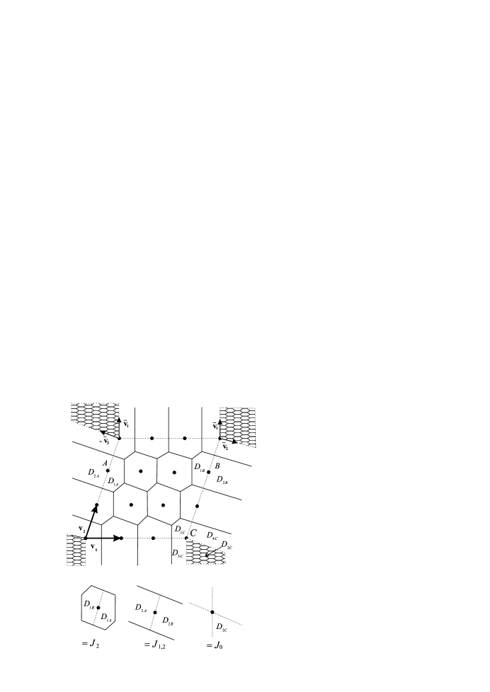
Figure 1: 2D Lattice and Decision Region Combining

For example, in Fig. 1, $\mathcal{S}_{1,1}=\{\mathbf{v_{1}}\}$ and $\mathcal{S}_{1,2}=\{\mathbf{v_{2}}\}$. We can decern two $\mathcal{F}_{1,1}$ edges parallel to $\mathbf{v_{1}}$, two $\mathcal{F}_{1,2}$ edges parallel to $\mathbf{v_{2}}$ and four vertices. There are four inner points lying in $\mathcal{F}_{2}$, two points on each equivalent $\mathcal{F}_{1,1}$ and $\mathcal{F}_{1,2}$ and four vertices in total. Points A and B are equivalent points according to Definition 7, since it is $u_{2}=2$ for both and they lie on equivalent $\mathcal{F}_{1,2}$ facets.

It must be noted here that the outer points of a finite lattice lying on a $\mathcal{F}_{k,p}$ facet, can also be considered as being points of a sublattice, defined by the basis vector subset $\mathcal{S}_{k,p}$. Accordingly, we define the following Voronoi cells:

Definition 8

The $k$-dimensional Voronoi cell of a sublattice, defined by a vector subset $\mathcal{S}_{k,p}$, is denoted by $\mathcal{V}_{\mathcal{S}_{k,p}}$. For $k=N$, $\mathcal{V}_{\mathcal{S}_{N}}\equiv\mathcal{V}_{\Lambda}$.

III Performance Evaluation in Additive White Gaussian Noise (AWGN)

In practical communication schemes using lattice constellations, the transmitted signal point belongs to a finite lattice constellation, as described in Section II-B. Next, the communication system model is presented and the geometry of these signal sets is examined.

III-A System Model

We consider communication in an AWGN channel where the received signal vector is

$$\mathbf{y}=\mathbf{x}+\mathbf{w},$$ (12)

with $\mathbf{y}\in\mathbb{R}^{N}$ being the received $N$-dimensional real signal vector, $\mathbf{x}\in\mathbb{R}^{N}$ is the transmitted $N$-dimensional real signal vector and $\mathbf{w}\in\mathbb{R}^{N}$ is the $N$-dimensional noise vector whose samples are zero-mean Gaussian independent random variables with variance $\sigma^{2}$. We define the signal-to-noise ratio (SNR) as $\rho=\frac{1}{\sigma^{2}}$. The transmitted signal vector $\mathbf{x}$ is a signal point in an infinite lattice constellation $\Lambda$ or a finite lattice constellation $\Lambda^{\prime}$.

The conditional probability of receiving $\mathbf{y}$ while transmitting $\mathbf{x}$ is

$$p(\mathbf{y}|\mathbf{x})=(2\pi\sigma^{2})^{-\frac{N}{2}}\exp\left(-\frac{1}{2\sigma^{2}}\|\mathbf{y}-\mathbf{x}\|^{2}\right),$$ (13)

and Maximum Likelihood (ML) detection is employed at the receiver.

III-B Analytical Expressions for the Symbol Error Probability (SEP)

In an infinite lattice constellation $\Lambda$, all signal points are considered equiprobable and they have exactly the same error performance since their Voronoi cells are equal. Thus the SEP of an infinite lattice constellation is [21]

$$P_{\infty}(\rho)=1-\int_{\mathcal{V}_{\Lambda}}p(\mathbf{z})\mathrm{d}\mathbf{z}.$$ (14)

The evaluation of $P_{\infty}(\rho)$ is often a tedious task due to the difficulty of the computation of $\mathcal{V}_{\Lambda}$ [13]. However, it can be approximated or bounded by closed-form expressions as in [21]. To the best of the authors’ knowledge, a similar expression to (14) for finite lattice constellations does not exist, since the decision regions of the outer points of these constellations do not lie in regions equal to $\mathcal{V}_{\Lambda}$, a fact often referred to as boundary effect [21].

The SEP of a finite lattice constellation is given by

$$P_{K-PAM}(\rho)=1-\frac{\sum\limits_{i=1}^{K^{N}}\left[\int_{\mathbf{R_{i}}}p(\mathbf{z})\mathrm{d}\mathbf{z}\right]}{K^{N}},$$ (15)

where $\mathbf{R_{i}}$, $i=1,\ldots,K^{N}$, are the regions of correct decision of the constellation signal points and $p(\mathbf{z})$ is the $N$-dimensional probability density function (pdf) of AWGN as defined in (13). The decision regions $\mathbf{R_{i}}$ of the inner points of the constellation are equal to the Voronoi cell $\mathcal{V}_{\Lambda}$, while those of the outer points are generally unknown. In order to circumvent this, we employ a geometrical technique, so as to express the sum of integrals in (15) in terms of integrals on integration regions that are Voronoi cells of the sublattices defined by the vector subsets $\mathcal{S}_{k,p}$.

To derive an analytical expression for (15), it is necessary first to proceed to a partitioning of the $N$-dimensional space in the following regions:

• The inner space of the parallelotope, $\mathcal{D}_{\mathcal{F}_{N}}\equiv\mathcal{F}_{N}$, as defined in (8).

• All the disjoint regions, denoted by $\mathcal{D}_{\mathcal{F}_{k,p}}$, which are the projections of a facet $\mathcal{F}_{k,p}$ to the directions vertical to this facet. These regions are defined as

  $$\begin{array}[]{cc}\mathcal{D}_{\mathcal{F}_{k,p}}=\{\mathbf{y}=\mathbf{x}+\overline{\mathbf{V}}\mathbf{a},\,\,\,\mathbf{a}\in\mathbb{R}^{N-k}_{+},\,\,\,\mathbf{x}\in\mathcal{F}_{k,p}\},&0\leq k<N,\end{array}$$ (16)

  where $\mathbf{x}$ are the points on a facet $\mathcal{F}_{k,p}$ as defined in (8), $\mathbf{a}$ is a vector of dimension $(N-k)\times 1$ with positive real elements and $\overline{\mathbf{V}}$ is an $N\times(N-k)$ matrix. If $k<(N-1)$, its columns are the vertical vectors on all $\mathcal{F}_{N-1,t}$ facets, which are adjacent to $\mathcal{F}_{k,p}$ according to Definition 4, with outward direction compared to the parallelotope. The number of $\mathcal{F}_{N-1,t}$ adjacent facets is $\binom{N-k}{q-k}$ for $q=N-1$, that is $\binom{N-k}{N-1-k}=\binom{N-k}{1}=N-k$. If $k=N-1$, then $\overline{\mathbf{V}}$ is an $N\times 1$ vector, vertical to the $\mathcal{F}_{N-1,p}$ facet itself, with outward direction compared to the parallelotope.

For example, in Fig. 1, the four partitions $\mathcal{D}_{\mathcal{F}_{0}}$ which are highlighted extend to infinity. Each corresponding matrix $\overline{\mathbf{V}}$ is a $2\times 2$ matrix containing the vectors $\overline{\mathbf{v_{1}}}$ and $\overline{\mathbf{v_{2}}}$, or their negatives, i.e. with opposite direction. Thus, an integral on the sum of these partitions equals an integral on the projection of one of the equivalent $\mathcal{F}_{0}$ facets to all directions vertical to it.

Remark 1

The outer points of a finite lattice constellation lie in decision regions which extend to the infinity. Taking into account that these regions are constructed by employing the ML criterion, for a signal point lying on a $\mathcal{F}_{k,p}$ facet, the decision region can be divided into partial regions. Each of them belongs ether to the inner space $\mathcal{D}_{\mathcal{F}_{N}}$, the region $\mathcal{D}_{\mathcal{F}_{k,p}}$ or the regions $\mathcal{D}_{\mathcal{F}_{q,t}}$, where $\mathcal{F}_{q,t}$ is a facet adjacent to $\mathcal{F}_{k,p}$, $q<N$. Consequently, for a point lying on some $\mathcal{F}_{k,p}$ with decision region $\mathbf{R}$ it holds that

$$\int_{\mathbf{R}}p(\mathbf{z})\mathrm{d}\mathbf{z}=\sum\limits_{i=k}^{N}\sum\limits_{j:\mathcal{S}_{k,p}\subseteq\mathcal{S}_{i,j}}\int_{D\in\mathcal{D}_{\mathcal{F}_{i,j}}}p(\mathbf{z})\mathrm{d}\mathbf{z},$$ (17)

where $D\in\mathcal{D}_{\mathcal{F}_{i,j}}$ is the part of the decision region in the partition $\mathcal{D}_{\mathcal{F}_{i,j}}$. The summation in (17) ensures that the facets considered are the facet $\mathcal{F}_{k,p}$ on which the point lies and all of its adjacent facets.

For example, in Fig. 1, point A lies on a $\mathcal{F}_{1,2}$ facet. According to Definition 4, the only adjacent facet to $\mathcal{F}_{1,2}$, is the inner space of the constellation $\mathcal{F}_{2}$. Thus, according to Remark 1, the decision region of A is divided in two parts, $D_{1A}$ and $D_{2A}$, with $D_{1A}\in\mathcal{D}_{\mathcal{F}_{2}}$ and $D_{2A}\in\mathcal{D}_{\mathcal{F}_{1,2}}$.

Definition 9

An integral $J_{k,p}$ is defined as

$$J_{k,p}=\int_{\mathcal{V}_{\mathcal{S}_{k,p}}}p(\mathbf{z_{k}})\mathrm{d}\mathbf{z_{k}},\,\,\,\,\,\,0<k<n,$$ (18)

where $p(\mathbf{z_{k}})$ is a $k$-dimensional zero mean Gaussian distribution, $\mathcal{V}_{\mathcal{S}_{k,p}}$ is the Voronoi cell of the k-dimensional sublattice defined by the basis vector subset $\mathcal{S}_{k,p}$. Note that when $k=0$, then $J_{0}\triangleq 1$.

Let $\mathcal{L}_{k,p}$ be the number of equivalent $\mathcal{F}_{k,p}$ facets for specific $k$ and $p$. If all the integrals on the decision regions of $\mathcal{L}_{k,p}$ equivalent $\mathcal{F}_{k,p}$-points are added, the resulting sum $\mathrm{S}$ is

$$\mathrm{S}=\sum\limits_{\mathcal{L}_{k,p}}\int_{\mathbf{R}}p(\mathbf{z})\mathrm{d}\mathbf{z}=\sum\limits_{\mathcal{L}_{k,p}}\sum\limits_{i=k}^{N}\sum\limits_{j:\mathcal{S}_{k,p}\subseteq\mathcal{S}_{i,j}}\int_{D\in\mathcal{D}_{\mathcal{F}_{i,j}}}p(\mathbf{z})\mathrm{d}\mathbf{z},$$ (19)

and since the decision regions $D\in\mathcal{D}_{\mathcal{F}_{i,j}}$ are disjoint for different points, (19) yields

$$\mathrm{S}=\sum\limits_{i=k}^{N}\sum\limits_{j:\mathcal{S}_{k,p}\subseteq\mathcal{S}_{i,j}}\int_{\sum\limits_{\mathcal{L}_{i,j}}D\in\mathcal{D}_{\mathcal{F}_{i,j}}}p(\mathbf{z})\mathrm{d}\mathbf{z},$$ (20)

where $\sum\limits_{\mathcal{L}_{i,j}}D\in\mathcal{D}_{\mathcal{F}_{i,j}}$ is the sum of partial decision regions of $\mathcal{L}_{k,p}$ equivalent points, on all $\mathcal{L}_{i,j}$ equivalent $\mathcal{F}_{i,j}$ facets. This sum of partial decision regions is a region which is the projection of a $\mathcal{V}_{\mathcal{S}_{i,j}}$ Voronoi cell to all directions vertical to the span of the $\mathcal{S}_{i,j}$ set of vectors. To reduce the integrals’ dimension, a change of variable and a Jacobian transformation is used, as in [19], and thus (20) yields

$$\mathrm{S}=\sum\limits_{i=k}^{N}\sum\limits_{j:\mathcal{S}_{k,p}\subseteq\mathcal{S}_{i,j}}\int_{\mathcal{V}_{\mathcal{S}_{k,p}}}p(\mathbf{z_{k}})\mathrm{d}\mathbf{z_{k}}=\sum\limits_{i=k}^{N}\sum\limits_{j:\mathcal{S}_{k,p}\subseteq\mathcal{S}_{i,j}}J_{i,j}.$$ (21)

For example, in Fig. 1, points A and B are equivalent points on $\mathcal{F}_{1,2}$ facets. Their decision regions are divided in the partial regions $D_{1A}$, $D_{2A}$, $D_{1B}$ and $D_{2B}$. The integrals on these partial regions are combined into two new integrals denoted with $J_{2}$ and $J_{1,2}$.

Employing the above method, we can now present the following theorem:

Theorem 1

The SEP of a multidimensional finite lattice constellation is given by

$$P_{K-PAM}(\rho)=1-\frac{\sum\limits_{k=0}^{N}(K-1)^{k}\sum\limits_{p=1}^{\binom{N}{k}}J_{k,p}}{K^{N}}.$$ (22)

Proof:

Due to Definition 4, Remark 1 and (21), the sum of partial regions of equivalent points, lying on all equivalent $\mathcal{F}_{k,p}$’s, for specific $k$ and $p$, yields the sum of integrals,

$$\mathrm{S}=\left\{\begin{array}[]{lc}\sum\limits_{i=k}^{N}\sum\limits_{j:\mathcal{S}_{k,p}\subseteq\mathcal{S}_{i,j}}J_{i,j},&k\neq 0,\\ \sum\limits_{i=0}^{N}\sum\limits_{j=1}^{\binom{N}{i}}J_{i,j},&k=0.\end{array}\right.$$ (23)

From (11) and (23), the sum of integrals of the regions of all points, lying on $\mathcal{F}_{k,p}$ facets for specific $k$ and $p$, is

$$\begin{array}[]{lc}(K-2)^{k}\sum\limits_{i=k}^{N}\sum\limits_{j:\mathcal{S}_{k,p}\subseteq\mathcal{S}_{i,j}}J_{i,j},&0<k<N,\\ \sum\limits_{i=0}^{N}\sum\limits_{j=1}^{\binom{N}{i}}J_{i,j},&k=0.\end{array}$$ (24)

Adding the above sums for all values of $p$ and $k$ we have

$$\sum_{k=1}^{N}\sum_{p=1}^{\binom{N}{k}}(K-2)^{k}\sum_{i=k}^{N}\sum_{j:\mathcal{S}_{k,p}\subseteq\mathcal{S}_{i,j}}J_{i,j}+\sum_{i=0}^{N}\sum_{j=1}^{\binom{N}{i}}J_{i,j}.$$ (25)

By changing the order of summing for indexes $i$ and $k$ in the first term of (25), and combining the sums for the enumeration indexes $p$ and $j$, due to the possible subsets and the times that each $J_{i,j}$ appears, (25) yields

$$\sum_{i=1}^{N}\sum_{k=1}^{i}\binom{i}{k}(K-2)^{k}\sum_{j=1}^{\binom{N}{i}}J_{i,j}+\sum_{i=0}^{N}\sum_{j=1}^{\binom{N}{i}}J_{i,j},$$ (26)

which can be written as

$$\sum_{i=0}^{N}\left(\sum_{k=0}^{i}\binom{i}{k}(K-2)^{k}-1\right)\sum_{j=1}^{\binom{N}{i}}J_{i,j}+\sum_{i=0}^{N}\sum_{j=1}^{\binom{N}{i}}J_{i,j},$$ (27)

or equivalently

$$\sum_{i=0}^{N}\sum_{k=0}^{i}\binom{i}{k}(K-2)^{k}\sum_{j=1}^{\binom{N}{i}}J_{i,j}.$$ (28)

Due to the binomial theorem, (28) reduces to

$$\sum\limits_{i=0}^{N}(K-1)^{i}\sum\limits_{j=1}^{\binom{N}{i}}J_{i,j}.$$ (29)

Using (29), (15) yields (22) and this concludes the proof. ∎

The expression in (22) cannot be directly evaluated, except for special cases, since the analytical evaluation of $\mathcal{V}_{\mathcal{S}_{k,p}}$ is generally a hard problem [13]. However, for the important case of SQAM constellations, since the Voronoi cells are square, (22) reduces to the well known closed-form SEP for the SQAM [24]. In the following we propose closed-form lower and upper bounds to $P_{K-PAM}\left(\rho\right)$, called Multiple Sphere Lower Bound (MSLB) and Multiple Sphere Upper Bound (MSUB), respectively. In these bounds, the integrals on the decision regions of the signal points are substituted by integrals on spheres of various dimensions.

III-C Multiple Sphere Lower Bound (MSLB)

For the readers’ convenience, we first present the Sphere Lower Bound (SLB) for infinite lattice constellations, presented also in [21].

The error probability, $P_{\infty}\left(\rho\right)$, of an infinite lattice constellation $\Lambda$ is lower-bounded by

$$P_{slb}(\rho)=1-\int\limits_{\mathcal{B}_{N}}p(\mathbf{z})\mathrm{d}\mathbf{z},$$ (30)

where $\mathcal{B}_{N}$ is an $N$-dimensional sphere of the same volume as the Voronoi cell $\mathcal{V}_{\mathcal{S}_{N}}$. Due to the normalization $|\mathrm{det}(\mathbf{M})|=1$, the sphere $\mathcal{B}_{N}$ is of unitary volume. It holds that [23]

$$\mathrm{vol}(\mathcal{B}_{N})=\frac{\pi^{\frac{N}{2}}R_{N}^{N}}{\Gamma\left(\frac{N}{2}+1\right)}=1,$$ (31)

where $R_{N}$ is the radius of the $N$-dimensional sphere, and $\Gamma(\cdot)$ is the Gamma Function defined by [25, Eq. (8.310)]. The radius $R_{N}$ is given by

$$R_{N}^{2}=\frac{1}{\pi}\Gamma\left(\frac{N}{2}+1\right)^{\frac{2}{N}}.$$ (32)

Subsequently, by substituting (32) in (30) and taking into account (13), we get

$$P_{slb}(\rho)=1-\int\limits_{\mathcal{B}_{N}}p(\mathbf{z})\mathrm{d}\mathbf{z}=1-\left[1-\frac{\Gamma\left(\frac{N}{2},\frac{R_{N}^{2}}{2}\rho\right)}{\Gamma\left(\frac{N}{2}\right)}\right]=\frac{\Gamma\left(\frac{N}{2},\frac{R_{N}^{2}}{2}\rho\right)}{\Gamma\left(\frac{N}{2}\right)},$$ (33)

where $\Gamma(a,x)=\int_{x}^{+\infty}t^{a-1}e^{-t}\mathrm{d}t$ is the upper incomplete Gamma function defined in [25, Eq. (8.350)].

Definition 10

We define the integrals

$$I_{k}=\int\limits_{\mathcal{B}_{k}}p(\mathbf{z_{k}})\mathrm{d}\mathbf{z_{k}},\,\,\,\,\,k=1,\ldots,N,$$ (34)

where $\mathcal{B}_{k}$ is a $k$-dimensional sphere of radius $R_{k}$ and $p(\mathbf{z_{k}})$ is a $k$-dimensional zero mean Gaussian distribution. When $k=0$, we define $I_{0}\triangleq J_{0}=1$.

The above integrals can be written as [21]

$$I_{k}=\left\{\begin{array}[]{cc}1,&k=0\\ 1-\frac{\Gamma\left(\frac{k}{2},\frac{R_{k}^{2}}{2}\rho\right)}{\Gamma\left(\frac{k}{2}\right)},&k=1,2,\ldots,N\\ \end{array}\right.$$ (35)

Similar to (32), with a slight modification for finite constellations, the radius $R_{k}$ in AWGN channels is defined as follows.

Definition 11

The sphere radius $R_{k}$ is given by

$$R_{k}^{2}=\left\{\begin{array}[]{cc}\frac{1}{\pi}\Gamma(\frac{k}{2}+1)^{\frac{2}{k}}W^{2},&k=1,2,\ldots,(N-1)\\ \frac{1}{\pi}\Gamma(\frac{k}{2}+1)^{\frac{2}{k}},&k=N\\ \end{array}\right.$$ (36)

where $W$ is

$$W=\frac{\|\mathbf{v_{1}}\|+\|\mathbf{v_{2}}\|+\ldots+\|\mathbf{v_{N}}\|}{N},$$ (37)

with $\|\mathbf{v_{i}}\|$ being the norm of basis vector $\mathbf{v_{i}}$. Note that for $\mathbb{Z}^{N}$ lattices, $W=1$.

Theorem 2

The SEP of a multidimensional finite lattice constellation is lower bounded by

$$P_{mslb}(\rho)=1-\frac{\sum\limits_{k=0}^{N}{(K-1)^{k}\binom{N}{k}I_{k}}}{K^{N}},$$ (38)

where $P_{mslb}(\rho)$ is called Multiple Sphere Lower Bound (MSLB).

Proof:

The volume of $\mathcal{V}_{\mathcal{S}_{k,p}}$ in (18), is the volume of Voronoi cell of a sublattice built by the basis vector subset $\mathcal{S}_{k,p}$. Since this volume is the same as the volume of the corresponding fundamental parallelotope of the sublattice, as a consequence of Hadamard’s inequality, it holds that

$$\mathrm{vol}_{k}(\mathcal{V}_{\mathcal{S}_{k,p}})\leq\prod_{i:\mathbf{v}_{i}\in\mathcal{S}_{k,p}}\|\mathbf{v}_{i}\|,$$ (39)

where the equality holds only when the vectors of $\mathcal{S}_{k,p}$ are orthogonal and $\mathrm{vol}_{k}(\cdot)$ is the $k$-dimensional volume of a region.

From (39) it is

$$\sum\limits_{p=1}^{\binom{N}{k}}\mathrm{vol}_{k}(\mathcal{V}_{\mathcal{S}_{k,p}})\leq\sum\limits_{p=1}^{\binom{N}{k}}\prod_{i:\mathbf{v}_{i}\in\mathcal{S}_{k,p}}\|\mathbf{v}_{i}\|,$$ (40)

which can be written as

$$\sum\limits_{p=1}^{\binom{N}{k}}\mathrm{vol}_{k}(\mathcal{V}_{\mathcal{S}_{k,p}})\leq\sum\limits_{\begin{subarray}{c}b_{1}+b_{2}+\ldots+b_{N}=k\\ b_{1},b_{2},\ldots,b_{N}\in\{0,1\}\end{subarray}}\|\mathbf{v}_{1}\|^{b_{1}}\|\mathbf{v}_{2}\|^{b_{2}}\cdots\|\mathbf{v}_{N}\|^{b_{N}}.$$ (41)

Using Maclaurin’s Inequality [26, p.52], for $a_{1},a_{2},\ldots,a_{N}\in\mathbb{R}$ and $0<k<N$,

$$\varrho_{N}^{\frac{1}{N}}\leq\varrho_{k}^{\frac{1}{k}}\leq\varrho_{1},$$ (42)

where

$$\varrho_{k}=\frac{\sum\limits_{\begin{subarray}{c}b_{1}+b_{2}+\ldots+b_{N}=k\\ b_{1},b_{2},\ldots,b_{N}\in\{0,1\}\end{subarray}}a_{1}^{b_{1}}a_{2}^{b_{2}}\cdots a_{N}^{b_{N}}}{\binom{N}{k}}.$$ (43)

If we set $a_{i}=\|\mathbf{v}_{i}\|$, $i=1,2,\ldots,N$, then $\varrho_{1}=W$ and from (42) and (43)

$$\sum\limits_{\begin{subarray}{c}b_{1}+b_{2}+\ldots+b_{N}=k\\ b_{1},b_{2},\ldots,b_{N}\in\{0,1\}\end{subarray}}\|\mathbf{v}_{1}\|^{b_{1}}\|\mathbf{v}_{2}\|^{b_{2}}\cdots\|\mathbf{v}_{N}\|^{b_{N}}\leq\binom{N}{k}W^{k}.$$ (44)

From (41) and (44), for $0<k<N$, we have

$$\sum\limits_{p=1}^{\binom{N}{k}}\mathrm{vol}_{k}(\mathcal{V}_{\mathcal{S}_{k,p}})\leq\binom{N}{k}W^{k}.$$ (45)

Due to the spherical symmetry of the AWGN pdf, it is

$$\int_{D}p(\mathbf{z_{k}})\mathrm{d}(\mathbf{z_{k}})\leq\int_{\mathcal{B}_{D}}p(\mathbf{z_{k}})\mathrm{d}\mathbf{z_{k}},$$ (46)

when $\mathrm{vol}_{k}(D)=\mathrm{vol}_{k}(\mathcal{B}_{D})$, as in [21]. In (46) $D$ is a random $k$-dimensional region of integration and $\mathcal{B}_{D}$ is a $k$-dimensional sphere of the same volume. Thus, from (18) and (46), it holds that

$$J_{k,p}=\int_{\mathcal{V}_{\mathcal{S}_{k,p}}}p(\mathbf{z_{k}})\mathrm{d}\mathbf{z_{k}}\leq\int_{\mathcal{B}(\mathcal{S}_{k,p})}p(\mathbf{z_{k}})\mathrm{d}\mathbf{z_{k}},$$ (47)

where $\mathcal{B}(\mathcal{S}_{k,p})$ is a sphere with volume $\mathrm{vol}_{k}\left(\mathcal{B}(\mathcal{S}_{k,p})\right)=\mathrm{vol}_{k}\left(\mathcal{V}_{\mathcal{S}_{k,p}}\right)$. Subsequently,

$$\sum\limits_{p=1}^{\binom{N}{k}}J_{k,p}\leq\sum\limits_{p=1}^{\binom{N}{k}}\int_{\mathcal{B}(\mathcal{S}_{k,p})}p(\mathbf{z_{k}})\mathrm{d}\mathbf{z_{k}}=\sum\limits_{p=1}^{\binom{N}{k}}\left(1-\frac{\Gamma\left(\frac{k}{2},\frac{R_{\mathcal{S}_{k,p}}^{2}}{2}\rho\right)}{\Gamma\left(\frac{k}{2}\right)}\right),$$ (48)

where $R_{\mathcal{S}_{k,p}}$ is the radius of the sphere $\mathcal{B}(\mathcal{S}_{k,p})$. From (45), and using that $\mathrm{vol}_{k}\left(\mathcal{B}(\mathcal{S}_{k,p})\right)=\frac{\pi^{\frac{k}{2}}R_{\mathcal{S}_{k,p}}^{k}}{\Gamma\left(\frac{k}{2}+1\right)}$ as in (31), it is

$$\sum\limits_{p=1}^{\binom{N}{k}}\frac{\pi^{\frac{k}{2}}R_{\mathcal{S}_{k,p}}^{k}}{\Gamma\left(\frac{k}{2}+1\right)}\leq\binom{N}{k}W^{k},$$ (49)

or by taking into account (36) for $0<k<N$,

$$\sum\limits_{m=1}^{\binom{N}{k}}R_{\mathcal{S}_{k,p}}^{k}\leq\binom{N}{k}R_{k}^{k}.$$ (50)

Now, if $a,b$ are positive real numbers, the function $f(x;a,b)=\Gamma\left(a,bx^{1/a}\right)$ is convex in $(0,\infty)$. Indeed

$$\frac{\partial{f}}{\partial{x}}=(bx^{1/a})^{a-1}e^{-bx^{1/a}}\frac{\partial{(bx^{1/a})}}{\partial{x}}=-\frac{b^{a}e^{-bx^{\frac{1}{a}}}}{a}$$ (51)

and

$$\frac{\partial^{2}{f}}{\partial{x^{2}}}=\frac{b^{a+1}x^{\frac{1}{a}-1}e^{-bx^{\frac{1}{a}}}}{a^{2}}>0,\,\,\forall x>0.$$ (52)

Thus from Jensen’s Inequality for convex functions [26]

$$\sum_{i=1}^{L}{\Gamma\left(a,b{x_{i}}^{1/a}\right)}\geq L\Gamma\left(a,b\left(\sum_{i=1}^{L}{x_{i}}/L\right)^{1/a}\right).$$ (53)

For $a=\frac{k}{2}$ , $b=\frac{\rho}{2}$, $L=\binom{N}{k}$ and $x_{i}={R^{k}_{\mathcal{S}_{k,p}}}$ we get

$$\sum_{p=1}^{\binom{N}{k}}{\Gamma\left(\frac{k}{2},\frac{\rho}{2}R^{2}_{\mathcal{S}_{k,p}}\right)}\geq\binom{N}{k}\Gamma\left(\frac{k}{2},\frac{\rho}{2}\left(\frac{\sum\limits_{m=1}^{\binom{N}{k}}R^{k}_{\mathcal{S}_{k,p}}}{\binom{N}{k}}\right)^{\frac{2}{k}}\right).$$ (54)

From (50) and since $f(x;a,b)=\Gamma\left(a,bx^{1/a}\right)$ is a decreasing function

$$\Gamma\left(\frac{k}{2},\frac{\rho}{2}\left(\frac{\sum\limits_{p=1}^{\binom{N}{k}}R^{k}_{\mathcal{S}_{k,p}}}{\binom{N}{k}}\right)^{\frac{2}{k}}\right)\geq\Gamma\left(\frac{k}{2},\frac{\rho}{2}R^{2}_{k}\right).$$ (55)

From (54) and (55), for $0<k<N$

$$\sum_{p=1}^{\binom{N}{k}}{\Gamma\left(\frac{k}{2},\frac{\rho}{2}R^{2}_{\mathcal{S}_{k,p}}\right)}\geq\binom{N}{k}\Gamma\left(\frac{k}{2},\frac{\rho}{2}R^{2}_{k}\right),$$ (56)

or equivalently

$$\sum_{p=1}^{\binom{N}{k}}\left(1-\frac{\Gamma\left(\frac{k}{2},\frac{\rho}{2}R^{2}_{\mathcal{S}_{k,p}}\right)}{\Gamma\left(\frac{k}{2}\right)}\right)\leq\binom{N}{k}\left(1-\frac{\Gamma\left(\frac{k}{2},\frac{\rho}{2}R^{2}_{k}\right)}{\Gamma\left(\frac{k}{2}\right)}\right).$$ (57)

Taking into account (48) and (57) for some $k$, $0<k<N$, it yields

$$\sum\limits_{p=1}^{\binom{N}{k}}J_{k,p}\leq\binom{N}{k}\left(1-\frac{\Gamma\left(\frac{k}{2},\frac{\rho}{2}R^{2}_{k}\right)}{\Gamma\left(\frac{k}{2}\right)}\right)=\binom{N}{k}I_{k},$$ (58)

while for $k=0$, $p=1$ and it holds that $J_{0}=I_{0}=1$.

For $k=N$, it is also $p=1$ and from (36) and (47)

$$J_{N}\leq\left(1-\frac{\Gamma\left(\frac{N}{2},\frac{\rho}{2}R^{2}_{N}\right)}{\Gamma\left(\frac{N}{2}\right)}\right)=I_{N}.$$ (59)

Combining (58)and (59), multiplying by $\left(K-1\right)^{k}$ and summing for all $k$, it yields

$$\sum\limits_{k=0}^{N}\left(K-1\right)^{k}\sum\limits_{p=1}^{\binom{N}{k}}J_{k,p}\leq\sum\limits_{k=0}^{N}\left(K-1\right)^{k}\binom{N}{k}I_{k}.$$ (60)

Using (22), (38) and (60),

$$P_{mslb}(\rho)\leq P(\rho)$$ (61)

and this concludes the proof. ∎

III-D Multiple Sphere Upper Bound (MSUB)

A well known upper bound for infinite lattice constellations, which is based on the minimum distance between signal points, is the Sphere Upper Bound (SUB) [13]

$$P_{sub}(\rho)=1-\int\limits_{\mathcal{G}_{N}}p(\mathbf{z})\mathrm{d}\mathbf{z},$$ (62)

where $\mathcal{G}_{N}$ is an $N$-dimensional sphere, with radius defined by

$$\mathcal{R}^{2}=\left(\frac{d_{min}}{2}\right)^{2}=\frac{d_{min}^{2}}{4},$$ (63)

with $d_{min}$ being the minimum distance on the infinite lattice constellation $\Lambda$. That is, the sphere $\mathcal{G}_{N}$ is inscribed in the Voronoi cell of the lattice.

When the generator matrix $\mathbf{M}$ is constructed by the basis vectors $\mathbf{v_{i}}$, $i=1,2,\ldots,N$ of the minimum possible norms, the minimum distance $d_{min}$ can be directly evaluated by $d_{min}=\min_{i}\left\|\mathbf{v_{i}}\right\|$. Although this is not always the case, the above is valid for the most commonly used lattices in practical cases, such as the $\mathbb{Z}^{N}$ lattices. Especially for the $\mathbb{Z}^{N}$ lattices, $d_{min}=1$.

The SUB in (62) can be rewritten as

$$P_{sub}(\rho)=1-\left[1-\frac{\Gamma\left(\frac{N}{2},\frac{\mathcal{R}^{2}}{2}\rho\right)}{\Gamma\left(\frac{N}{2}\right)}\right]=\frac{\Gamma\left(\frac{N}{2},\frac{\mathcal{R}^{2}}{2}\rho\right)}{\Gamma\left(\frac{N}{2}\right)}.$$ (64)

Similarly, based on (22) and in the same concept as the SUB for infinite lattice constellations, we can now provide a novel upper bound for finite lattice constellations.

Definition 12

We define the integrals

$$\mathcal{I}_{k}=\int\limits_{\mathcal{G}_{k}}p(\mathbf{z_{k}})\mathrm{d}\mathbf{z_{k}},\,\,\,\,\,k=0,1,\ldots,N,$$ (65)

where $\mathcal{G}_{k}$ is a $k$-dimensional sphere, with radius defined in (63). When $k=0$, we define $\mathcal{I}_{0}=J_{0}=1$.

The above integrals can be written as [21]

$$\mathcal{I}_{k}=\left\{\begin{array}[]{cc}1,&k=0\\ 1-\frac{\Gamma\left(\frac{k}{2},\frac{\mathcal{R}^{2}}{2}\rho\right)}{\Gamma\left(\frac{k}{2}\right)},&k=1,2,\ldots,N.\\ \end{array}\right.$$ (66)

Theorem 3

The SEP of a multidimensional finite lattice constellation is upper bounded by

$$P_{msub}(\rho)=1-\frac{\sum\limits_{k=0}^{N}{(K-1)^{k}\binom{N}{k}\mathcal{I}_{k}}}{K^{N}},$$ (67)

where $P_{msub}(\rho)$ is called Multiple Sphere Upper Bound (MSUB).

Proof:

If $d_{min}(\mathcal{S}_{k,p})$ is the minimum distance between signal points on the sublattice defined by the basis vector subset $\mathcal{S}_{k,p}$, for any $J_{k,p}$, computed on a Voronoi cell $\mathcal{V}_{\mathcal{S}_{k,p}}$

$$J_{k,p}=\int_{\mathcal{V}_{\mathcal{S}_{k,p}}}p(\mathbf{z_{k}})\mathrm{d}\mathbf{z_{k}}\geq\int_{\mathcal{G}(\mathcal{S}_{k,p})}p(\mathbf{z_{k}})\mathrm{d}\mathbf{z_{k}},$$ (68)

where $\mathcal{G}(\mathcal{S}_{k,p})$ is a $k$-dimensional sphere with radius $\mathcal{R}_{\mathcal{S}_{k,p}}=\frac{d_{min}(\mathcal{S}_{k,p})}{2}$. The sphere $\mathcal{G}(\mathcal{S}_{k,p})$ is inscribed in the Voronoi cell $\mathcal{V}_{\mathcal{S}_{k,p}}$. It is generally valid that $d_{min}(\mathcal{S}_{k,p})\geq d_{min}$, where $d_{min}$ is the minimum distance on the lattice defined by the basis vector set $\mathcal{S}_{N}$. This is straightforward, since $\mathcal{S}_{k,p}\subseteq\mathcal{S}_{N}$.

Thus,

$$\int_{\mathcal{G}(\mathcal{S}_{k,p})}p(\mathbf{z_{k}})\mathrm{d}\mathbf{z_{k}}\geq\int_{\mathcal{G}_{k}}p(\mathbf{z_{k}})\mathrm{d}\mathbf{z_{k}},$$ (69)

where $\mathcal{G}_{k}$ is a $k$-dimensional sphere with radius $\mathcal{R}=\frac{d_{min}}{2}$, as defined in (63). The sphere $\mathcal{G}_{k}$ is always smaller or at the most equal to the inscribed sphere of the Voronoi cell $\mathcal{V}_{\mathcal{S}_{k,p}}$.

Taking into account (65), (68) and (69), it is $J_{k,p}\geq\mathcal{I}_{k}$ and subsequently,

$$\sum\limits_{k=0}^{N}\left(K-1\right)^{k}\sum\limits_{p=1}^{\binom{N}{k}}J_{k,p}\geq\sum\limits_{k=0}^{N}\left(K-1\right)^{k}\binom{N}{k}\mathcal{I}_{k}.$$ (70)

From (22), (67) and (70),

$$P_{msub}(\rho)\geq P(\rho)$$ (71)

and this concludes the proof. ∎

IV Numerical Results & Discussion

In this section we illustrate the accuracy and tightness of the proposed lower and upper bounds, MSLB and MSUB, respectively, in comparison with the SEP, as approximated by Monte-Carlo simulation, for various finite lattice constellations in AWGN channels. We also compare the MSLB and MSUB with the existing bounds for the infinite lattice constellations, the SLB and SUB. The lattice constellations most commonly used in practical cases are those carved from $\mathbb{Z}^{N}$ lattices, due to the easy Gray coded bit labeling. In the following, apart from $\mathbb{Z}^{N}$ lattices, the $\mathbb{A}^{2}$, $\mathbb{E}^{4}$ and $\mathbb{E}^{8}$ are also illustrated, as an example of lattice structures different from the orthogonal constellations. These schemes usually achieve better SEP but they cannot be labeled with a Gray code.

Fig. 2 illustrates the performance of a $\mathbb{Z}^{2}$ 4-PAM constellation, which is a simple case of lattice constellations, most commonly named as 16-Square Quadrature Amplitude Modulation (16-SQAM). The simulated SEP of the constellation in the AWGN channel is plotted in conjunction with the corresponding MSLB and MSUB for various values of the SNR, $\rho=\frac{1}{\sigma^{2}}$. For the $\mathbb{Z}^{N}$ lattices, the generator matrix is $\mathbf{M}=\mathbf{I}_{N}$, where $\mathbf{I}_{N}$ is the $N\times N$ identity matrix, while $W=d_{min}=1$. It is evident that the MSLB acts as a lower bound, while the MSUB acts as an upper bound, for all values of $\rho$. Both bounds are very tight and can be effectively used to assess the performance of the $\mathbb{Z}^{2}$ 4-PAM constellation. Compared to the existing SLB, the proposed MSLB corresponds better to the actual performance of the constellation. Furthermore it is evident that the SLB does not act as a lower bound for SNR values lower than $15$dB, whereas the SLB becomes less tight than the MSLB for SNR values higher than $17$dB. Finally, although the existing SUB is an upper bound to the actual performance, the MSUB is almost $0.5$dB tighter than the SUB.

Fig. 3 shows the performance of a $\mathbb{Z}^{2}$ 32-PAM constellation. It is clearly illustrated that both the MSLB and the MSUB bound the performance of the lattice and they are still very tight, even if the rank of the $K$-PAM increases. In this situation, the MSLB is almost in accordance with the SLB, and the MSUB with the SUB respectively. This is because the inner points are approximated in the same way and the ratio inner/outer points on the constellation is higher than that of the 4-PAM constellation. This implies that, for a specific dimension $N$, as $K$ increases, the MSLB converges to the corresponding SLB, and the MSUB converges to the SUB.

Figs. 4 and 5 depict the performance of a $\mathbb{Z}^{4}$ 4-PAM and a $\mathbb{Z}^{8}$ 4-PAM respectively, together with the corresponding MSLBs, MSUBs, SLBs and SUBs. Comparing with Fig. 2, where a $\mathbb{Z}^{2}$ 4-PAM is illustrated, it is evident that, for a specific $K$, as the dimension decreases, the bounds become more tight. Still, for both dimensions, the proposed bounds are tighter than the existing SLBs and SUBs, while for the SLB we can also see that for low SNR values, it does not act as a bound. Moreover, since MSLB and SLB diverge from each other for high SNR values, the results also suggest that the MSLB has different diversity order than the SLB, corresponding better to the diversity order of the actual performance of the constellations.

In the following figures, the performance of some non orthogonal lattices is depicted, in order to highlight the efficiency of the MSLB and MSUB for various lattice structures. In Fig. 6, a $\mathbb{A}^{2}$ 4-PAM is illustrated. The generator matrix is given by [23]

$$\mathbf{M}=\left[\begin{array}[]{cc}\sqrt{\frac{2}{\sqrt{3}}}&\sqrt{\frac{1}{2\sqrt{3}}}\\ 0&\sqrt{\frac{3}{2\sqrt{3}}}\end{array}\right],$$ (72)

and thus $W=\sqrt{\frac{2}{\sqrt{3}}}$ and $d_{min}=\sqrt{\frac{2}{\sqrt{3}}}$. Once again it is clear that both the MSLB and MSUB are reliable and tight, in constrast to the SLB and SUB. Specifically, the corresponding SLB is not a lower bound for this case, for all SNR values considered. Moreover, the proposed bounds are more tight than the case of $\mathbb{Z}^{N}$ lattices. This can be attributed to the structure of the $\mathbb{A}^{2}$ lattice, since the Voronoi cells of these lattices are regular polytopes, which are better approximated by the spheres, used both in MSLB and MSUB.

In Fig. 7, the rank $K$ of the $\mathbb{A}^{2}$ lattice is increased from $K=4$ to $K=32$. Again, as $K$ increases, MSLB and MSUB converge to the corresponding SLB and SUB, maintaining their accuracy and tightness.

In Figs. 8 and 9, the lattices $\mathbb{E}^{4}$ 4-PAM and $\mathbb{E}^{8}$ 4-PAM are presented [23, 27]. The generator matrices are given in (73), while $W=d_{min}=\frac{2}{8^{\frac{1}{4}}}$ for $N=4$, and $W=\frac{2+7\sqrt{2}}{8}$ and $d_{min}=\sqrt{2}$ for $N=8$. Both MSLB and MSUB act as tight bounds, in contrast to the corresponding SLB and SUB, while they are tighter than the corresponding cases of the $\mathbb{Z}^{N}$ lattices.

$$\mathbf{M}_{\mathbb{E}^{4}}=\frac{1}{8^{\frac{1}{4}}}\left[\begin{array}[]{cccc}1&2&0&0\\ 1&0&2&0\\ 1&0&0&2\\ 1&0&0&0\end{array}\right],\,\,\,\,\,\,\,\,\,\mathbf{M}_{\mathbb{E}^{8}}=\left[\begin{array}[]{cccccccc}2&-1&0&0&0&0&0&1/2\\ 0&1&-1&0&0&0&0&1/2\\ 0&0&1&-1&0&0&0&1/2\\ 0&0&0&1&-1&0&0&1/2\\ 0&0&0&0&1&-1&0&1/2\\ 0&0&0&0&0&1&-1&1/2\\ 0&0&0&0&0&0&1&1/2\\ 0&0&0&0&0&0&0&1/2\end{array}\right].$$ (73)

V Conclusions

We studied the error performance of finite lattice constellations via a combinatorial geometrical approach. First we presented an analytical expression for the exact SEP of these signal sets, which is then used to introduce two novel closed-form bounds, called Multiple Sphere Lower Bound (MSLB) and Multiple Sphere Upper Bound (MSUB). The accuracy and tightness of MSLB and MSUB have been illustrated in comparison with the simulated SEP of various constellations of different lattice structure, dimension and rank. The proposed bounds are tighter to the actual performance, compared to the SLB and SUB which are often used as approximations for the finite case. The presented approach can be extended to multidimensional signal sets distorted by fading, as presented in Part II. Since these constellations illustrate substantial diversity gains, the proposed analytical framework and its extension to fading channels becomes an important and efficient tool for their design and performance evaluation.

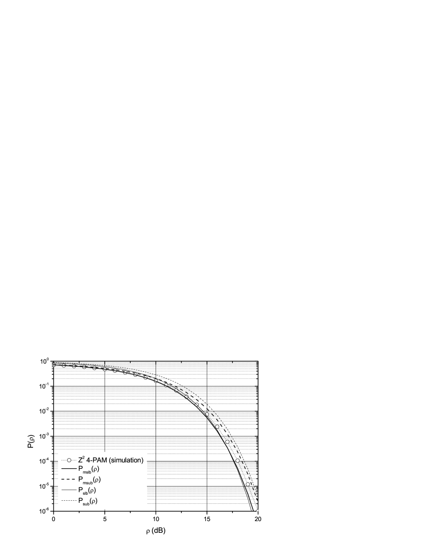
Figure 2: Symbol Error Probability, MSLB and MSUB for the $\mathbb{Z}^{2}$ $4-PAM$ constellation and SLB and SUB for the $\mathbb{Z}^{2}$ lattice.

Figure 3: Symbol Error Probability, MSLB and MSUB for the $\mathbb{Z}^{2}$ $32-PAM$ constellation and SLB and SUB for the $\mathbb{Z}^{2}$ lattice.

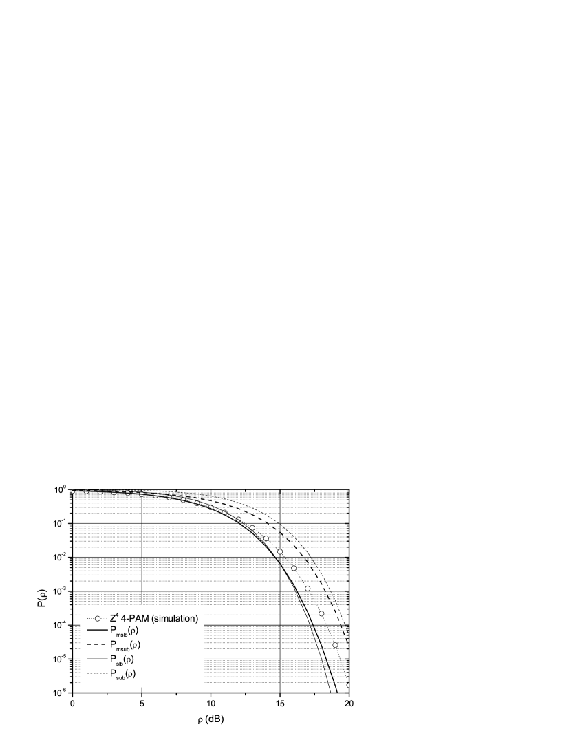
Figure 4: Symbol Error Probability, MSLB and MSUB for the $\mathbb{Z}^{4}$ $4-PAM$ constellation and SLB and SUB for the $\mathbb{Z}^{4}$ lattice.

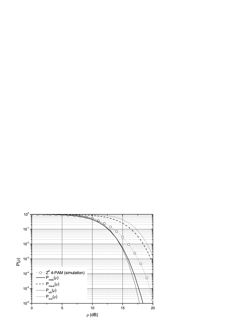
Figure 5: Symbol Error Probability, MSLB and MSUB for the $\mathbb{Z}^{8}$ $4-PAM$ constellation and SLB and SUB for the $\mathbb{Z}^{8}$ lattice.

Figure 6: Symbol Error Probability, MSLB and MSUB for the $\mathbb{A}^{2}$ $4-PAM$ constellation and SLB and SUB for the $\mathbb{A}^{2}$ lattice.

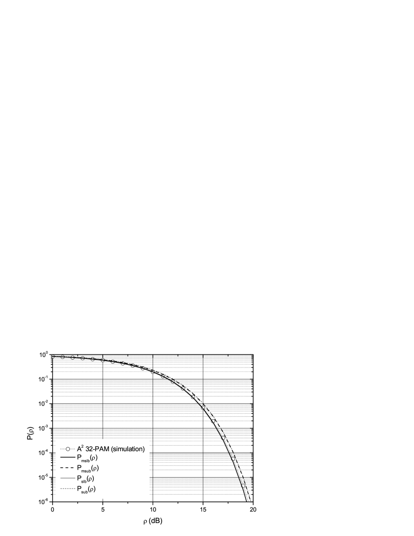
Figure 7: Symbol Error Probability, MSLB and MSUB for the $\mathbb{A}^{2}$ $32-PAM$ constellation and SLB and SUB for the $\mathbb{A}^{2}$ lattice.

Figure 8: Symbol Error Probability, MSLB and MSUB for the $\mathbb{E}^{4}$ $4-PAM$ constellation and SLB and SUB for the $\mathbb{E}^{4}$ lattice.

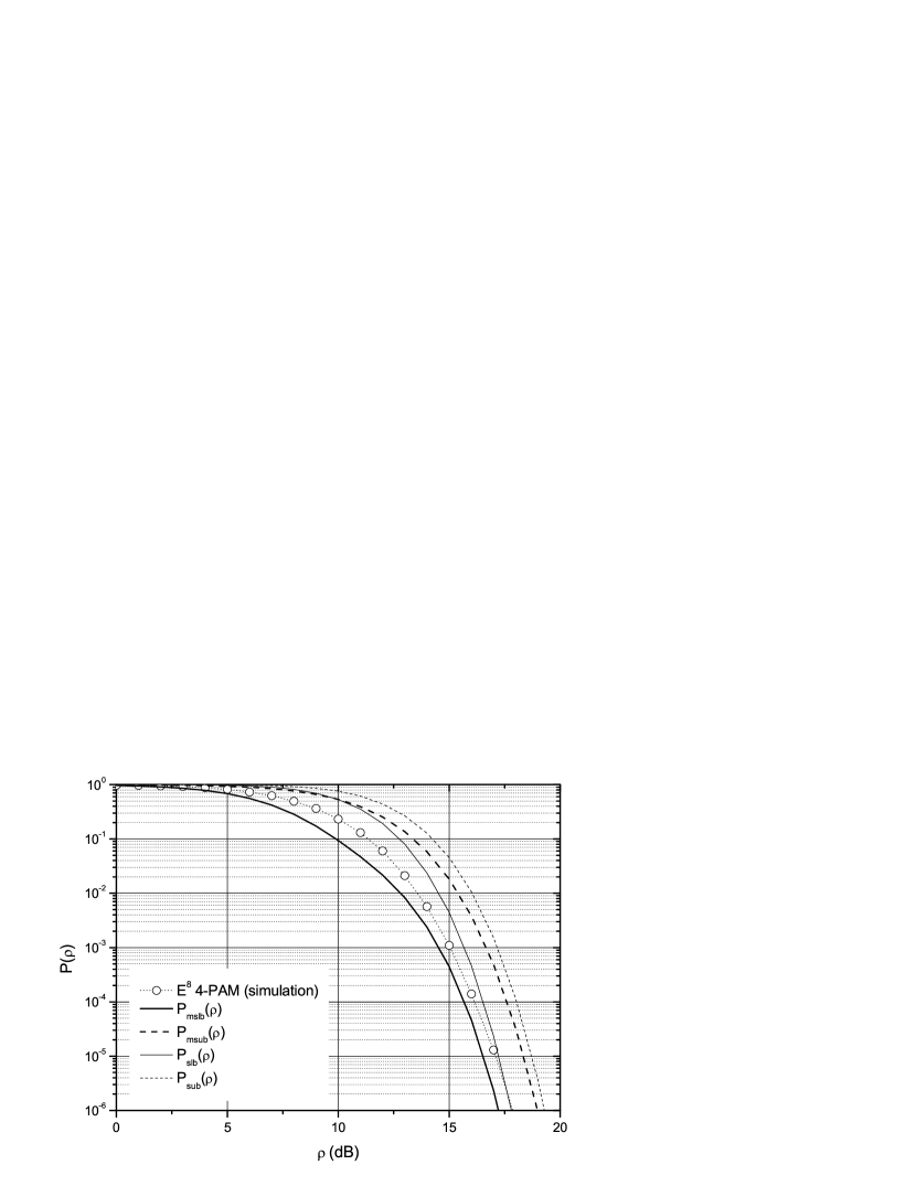
Figure 9: Symbol Error Probability, MSLB and MSUB for the $\mathbb{E}^{8}$ $4-PAM$ constellation and SLB and SUB for the $\mathbb{E}^{8}$ lattice.

References

- [1] J. Boutros and E. Viterbo, “Signal Space Diversity: A power- and bandwidth-efficient diversity technique for the Rayleigh fading channel”, IEEE Trans. Inf. Theory, vol. 44, no. 4, p. 1453–1467, Jul. 1998.
- [2] J. Boutros, E. Viterbo, C. Rastello, and J. C. Belfiore, “Good lattice constellations for both Rayleigh fading and Gaussian channels”, IEEE Trans. Inf. Theory, vol. 42, no. 2 pp. 502–518, Mar. 1996.
- [3] X. Giraud, E. Boutillon, and J. C. Belfiore, “Algebraic tools to build modulation schemes for fading channels”, IEEE Trans. Inf. Theory, vol. 43, no. 3, pp. 938-952, May 1997.
- [4] E. Bayer-Fluckiger, F. Oggier, and E. Viterbo, “New algebraic constructions of rotated Zn-lattice constellations for the Rayleigh fading channel,” IEEE Trans. Inf. Theory, vol. 50, no. 4, pp. 702–714, Apr. 2004.
- [5] F. Oggier and E. Viterbo, Algebraic Number Theory And Code Design For Rayleigh Fading Channels, Foundations and Trends in Communications and Information Theory, Now Publishers Inc, 2004.
- [6] H. Lee and A. Paulraj, “MIMO Systems Based on Modulation Diversity,”IEEE Trans. Commun., vol.58, no.12, pp.3405-3409, December 2010.
- [7] F. Kharrat-Kammoun, S. Fontenelle, and J. Boutros, “Accurate Approximation of QAM Error Probability on Quasi-Static MIMO Channels and Its Application to Adaptive Modulation,”IEEE Trans. Inf. Theory, vol.53, no.3, pp.1151-1160, March 2007.
- [8] S.A. Ahmadzadeh, S.A. Motahari, and A.K.Khandani, “Signal space cooperative communication,”IEEE Trans. Wireless Commun., vol.9, no.4, pp.1266-1271, April 2010.
- [9] Y. Li, X.-G. Xia, G. Wang,“Simple iterative methods to exploit the signal-space diversity,”IEEE Trans. Commun., vol.53, no.1, pp. 32- 38, Jan. 2005.
- [10] H. Lee, J. Cho, J.-K. Kim, and I. Lee, “Real-domain decoder for full-rate full-diversity STBC with multidimensional constellations,”IEEE Trans. Commun.,vol.57, no.1, pp.17-21, January 2009.
- [11] N.H. Tran, H.H. Nguyen, and T. Le-Ngoc, “Performance of BICM-ID with Signal Space Diversity,”IEEE Trans. Wireless Commun., vol.6, no.5, pp.1732-1742, May 2007.
- [12] Framing Structure, Channel Coding and Modulation for a Second Generation Digital Terrestrial Television Broadcasting System (DVB-T2), ETSI EN 302 755 V.1.2.1, Feb. 2011.
- [13] E. Viterbo and E. Biglieri, “Computing the Voronoi cell of a lattice: the diamond-cutting algorithm,” IEEE Trans. Inf. Theory, vol. 42, no. 1, p. 161–171, Jan. 1996.
- [14] J.-C. Belfiore and E. Viterbo, “Approximating the error probability for the independent Rayleigh fading channel”, in Proc. 2005 International Symposium on Information Theory, Adelaide, Australia, Sept. 2005.
- [15] G. Taricco and E. Viterbo, “Performance of high-diversity multidimensional constellations”, IEEE Trans. Inf. Theory, vol. 44, no. 4, pp. 1539-1543, Jul 1998.
- [16] E. Bayer-Fluckiger, F. Oggier, and E. Viterbo, “Algebraic lattice constellations: bounds on performance,”IEEE Trans. Inf. Theory, vol.52, no.1, pp. 319- 327, Jan. 2006.
- [17] J. Kim, W. Lee, J.-K. Kim, and I. Lee, “On the symbol error rates for signal space diversity schemes over a Rician fading channel”, IEEE Trans. Commun., vol. 57, no. 8, pp. 2204-2209, Aug. 2009.
- [18] C. E. Shannon, “Probability of error for optimal codes in a Gaussian channel”, The Bell Syst. Techn. J., vol. 38, no. 3, pp. 279–324, May 1959
- [19] V. Tarokh, A. Vardy, and K. Zeger, “Universal bound on the performance of lattice codes,” IEEE Trans. Inf. Theory, vol. 45, no. 2, pp. 670–681, Mar. 1999.
- [20] S. Vialle and J. Boutros, “Performance of optimal codes on Gaussian and Rayleigh fading channels: a geometrical approach”, in Proc. 37th Allerton Conf. on Commun., Control and Comput., Monticello, IL, Sept. 1999.
- [21] A. G. Fàbregas and E. Viterbo, “Sphere lower bound for rotated lattice constellations in fading channels”, IEEE Trans. Wireless Commun., vol. 7, no. 3, p. 825-830, Mar. 2008.
- [22] K. N. Pappi, N. D. Chatzidiamantis and G. K. Karagiannidis, “Error Performance of Multidimensional Lattice Constellations - Part II: Evaluation in Fading Channels”, submitted to IEEE Trans. Commun.
- [23] J. H. Conway and N. J. A. Sloane, Sphere Packings, Lattices and Groups, 3rd ed. Springer, 1999.
- [24] J. G. Proakis, Digital Communications, 4th ed. New York: McGraw-Hill, 2001.
- [25] I. S. Gradshteyn and I. M. Ryzhik, Table of Integrals, Series, and Products, New York, Academic Press, 7th edition, 2007.
- [26] G.H. Hardy, J.E. Littlewood, and G. Polya, Inequalities, 2nd ed. Cambridge, UK, Cambridge Univ. Press, 1952.
- [27] T.M. Thompson, From Error-Correcting Codes Through Sphere Packings to Simple Groups (Carus Mathematical Monographs), The Mathematical Association of America, USA, 1983.