Error Performance of Multidimensional Lattice Constellations - Part II: Evaluation over Fading Channels

Abstract

This is the second part of a two-part series of papers, where the error performance of multidimensional lattice constellations with signal space diversity (SSD) is investigated. In Part I, following a novel combinatorial geometrical approach which is based on parallelotope geometry, we have presented an exact analytical expression and two closed-form bounds for the symbol error probability (SEP) in Additive White Gaussian Noise (AWGN). In the present Part II, we extend the analysis and present a novel analytical expression for the Frame Error Probability (FEP) of multidimensional lattice constellations over Nakagami-$m$ fading channels. As the FEP of infinite lattice constellations is lower bounded by the Sphere Lower Bound (SLB), we propose the Sphere Upper Bound (SUB) for block fading channels. Furthermore, two novel bounds for the FEP of multidimensional lattice constellations over block fading channels, named Multiple Sphere Lower Bound (MSLB) and Multiple Sphere Upper Bound (MSUB), are presented. The expressions for the SLB and SUB are given in closed form, while the corresponding ones for MSLB and MSUB are given in closed form for unitary block length. Numerical and simulation results illustrate the tightness of the proposed bounds and demonstrate that they can be efficiently used to set the performance limits on the FEP of lattice constellations of arbitrary structure, dimension and rank.

I Introduction

The performance evaluation of multidimensional signal sets has attracted significant attention due to the signal space diversity (SSD) that these constellations present [2] and the fact that they can be efficiently used to combat the signal degradation caused by fading. The design of such constellations has been extensively studied in [3, 4, 5, 6], but since the analytical computation of the Voronoi cells of multidimensional constellations is difficult[7], their error performance has been evaluated only through approximations and bounds [8, 9, 10], while for special cases, some exact but complicated analytical expressions were derived [11].

In Part I [1] of this two-part series of papers, based on parallelotope geometry we introduced a novel combinatorial geometrical approach for the evaluation of the error performance of multidimensional lattice constellations in Additive White Gaussian Noise (AWGN). Especially, we proposed an exact analytical expression for the Symbol Error Probability (SEP) of these signal sets and two novel closed-form bounds, namely the Multiple Sphere Lower Bound (MSLB) and the Multiple Sphere Upper Bound (MSUB). With the introduction of the MSLB in part I, the concept of the Sphere Lower Bound (SLB) was extended to the case of finite signal sets. The SLB dates back to Shannon’s work [12] and although it has been thoroughly investigated in the literature [7, 13, 14, 15], it is not generally a reliable lower bound for the important practical cases of finite lattice constellations. Moreover, a similar upper bound, the Sphere Upper Bound (SUB) has been investigated in [7] for AWGN channels.

I-A Contribution

In the present Part II, we study the error performance of multidimensional infinite and finite lattice constellations in Nakagami-$m$ block fading channels. Specifically, for infinite lattice constellations:

• We propose a novel expression for the SUB which is suitable for the analysis in fading channels while it upper bounds the Frame Error Probability (FEP).

• We present novel closed-form expressions for the well known SLB and the proposed SUB in Nakagami-m block fading channels.

For multidimensional lattice constellations, based on the proposed expressions for the exact SEP, the MSLB and MSUB in AWGN given in Part I [1]:

• We present a novel analytical expression for the Frame Error Probability (FEP) of finite lattice constellations in the presence of Nakagami-m block fading.

• Starting from this expression we propose alternative formulae for the MSLB and the MSUB which are suitable for the performance analysis in fading channels and bound the FEP.

• We present closed-form expressions for the MSLB and MSUB in Nakagami-m block fading channels for the case of unitary block length.

I-B Structure

The remainder of the paper is organized as follows. In Section II, the channel model and the characteristics of faded lattices are presented. Section III investigates the exact FEP of infinite and finite lattice constellations, while the SLB, MSLB, SUB and MSUB for block fading are presented and their closed-form expressions are proposed. Section IV illustrates the accuracy and tightness of the proposed bounds via extensive numerical and simulation results, whereas conclusions are discussed in Section V.

I-C Notations

Here, we revisit some symbols and terms defined in Part I [1] and also used in Part II:

• $\Lambda$ denotes an infinite lattice constellation and $\Lambda^{\prime}$ a finite lattice constellation, carved from a lattice $\Lambda$.

• $N$ denotes the dimension of a lattice or lattice constellation.

• $\mathbf{M}$ denotes a generator matrix of a lattice $\Lambda$, where $\mathbf{M}=\left[\mathbf{v}_{1}~{}\mathbf{v}_{2}...\mathbf{v}_{N}\right]$, $\mathbf{M}\in\mathbb{R}^{N\times N}$ and $|\mathrm{det}(\mathbf{M})|=1$. Vectors $\mathbf{v}_{i}$, $i=1,2,\ldots,N$, are the basis vectors of the lattice.

• $K$ is the number of symbols along the direction of each basis vector.

• $\mathcal{S}_{N}$ denotes the set of the basis vectors of the $N$-dimensional lattice and $\mathcal{S}_{k,p}$ is a subset of $k$ out of $N$ basis vectors, with $p$ an index enumerating the different possible subsets for each $k$. For specific $k$, the index is $p=1,\ldots,\binom{N}{k}$.

• $\mathcal{V}_{\mathcal{S}_{k,p}}$ denotes the Voronoi cell of the sublattice, defined by the vector subset $\mathcal{S}_{k,p}$.

• $\mathrm{vol}_{k}(\cdot)$ is the volume of a $k$-dimensional geometrical region. Note that $\mathrm{vol}_{N}\left(\mathcal{V}_{\mathcal{S}_{N}}\right)=|\mathrm{det}(\mathbf{M})|=1$.

• $d_{min}$ is the minimum distance between two points in an infinite or in a finite lattice constellation.

II System Model

II-A Channel Model

Let us consider a flat fading channel whose discrete time received vector is given by

$$\mathbf{y}_{l}=\mathbf{Hx}_{l}+\mathbf{z}_{l},~{}~{}l=1,...,L,$$ (1)

where $\mathbf{y}_{l}\in\mathbb{R}^{N}$ is the $N$-dimensional real received signal vector, $\mathbf{x}_{l}\in\mathbb{R}^{N}$ is the $N$-dimensional real transmitted signal vector, $\mathbf{H}=$diag$\left(\mathbf{h}\right)\in\mathbb{R}^{N\times N}$ is the flat fading diagonal matrix with $\mathbf{h}=\left(h_{1},...,h_{N}\right)\in\mathbb{R}^{N}$, and $\mathbf{z}_{l}\in\mathbb{R}^{N}$ is the Additive White Gaussian Noise (AWGN) vector whose samples are zero-mean Gaussian independent random variables with variance $\sigma^{2}$. Furthermore, $L$ denotes the number of $N$-dimensional modulation symbols in one frame.

The fading matrix $\mathbf{H}$ is assumed to be constant during one frame and changes independently from frame to frame, i.e., block fading channel with $N$ blocks is considered. Thus, for a given channel realization, the channel transition probabilities are given by

$$p\left(\mathbf{y}\left|\mathbf{x},\mathbf{H}\right.\right)=\left(2\pi\sigma^{2}\right)^{-\frac{N}{2}}\exp\left(-\frac{1}{2\sigma^{2}}\left\|\mathbf{y}-\mathbf{Hx}\right\|^{2}\right).$$ (2)

Moreover, it is assumed that the real fading coefficients, $h_{i}$ for $i=1,...,N,$ follow Nakagami-$m$ distribution [16], with probability density function (pdf) given by

$$p_{h_{i}}\left(x\right)=\frac{2m^{m}x^{2m-1}}{\Gamma\left(m\right)}\exp\left(-mx^{2}\right),$$ (3)

while the coefficients, $\gamma_{i}=h_{i}^{2}$, that correspond to the fading power gains and will be used in the following analysis, are Gamma distributed with pdf

$$p_{\gamma_{i}}\left(x\right)=\frac{m^{m}x^{m-1}}{\Gamma\left(m\right)}\exp\left(-mx\right)$$ (4)

and cumulative density function (cdf)

$$P_{\gamma_{i}}\left(x\right)=1-\frac{\Gamma\left(m,mx\right)}{\Gamma\left(m\right)}.$$ (5)

In the above equations, $m\geq 0.5$ and $\Gamma\left(\cdot\right)$, $\Gamma\left(\cdot,\cdot\right)$ denote the Gamma [17, Eq. (8.310)] and the upper incomplete Gamma [17, Eq. (8.310)] functions, respectively. Finally, the signal-to-noise ratio (SNR) is defined as $\rho=\frac{1}{\sigma^{2}}$.

II-B Faded Lattices

As described in Part I, the transmitted signal vectors $\mathbf{x}$ belong to an $N$-dimensional infinite or finite lattice constellation, defined respectively as [1, Eq. (1)] [1, Eq. (5)]

$$\Lambda=\mathbf{M}\mathbf{z},\,\,\,\,\,\,\,\,\mathbf{z}\in\mathbb{Z}^{N},$$ (6)

and

$$\begin{array}[]{ccc}\Lambda^{\prime}=\mathbf{M}\mathbf{u},&\mathbf{u}=[u_{1}\,\,u_{2}\,\,\ldots\,\,u_{N}]^{T},&u_{i}\in\{0,1,\ldots,K-1\}.\end{array}$$ (7)

Similarly, the faded infinite or finite lattice constellation is defined as the lattice seen by the receiver which is given by

$$\Lambda_{f}=\mathbf{H}\mathbf{M}\mathbf{z},\,\,\,\,\,\,\,\,\mathbf{z}\in\mathbb{Z}^{N},$$ (8)

and

$$\begin{array}[]{ccc}\Lambda^{\prime}_{f}=\mathbf{H}\mathbf{M}\mathbf{u},&\mathbf{u}=[u_{1}\,\,u_{2}\,\,\ldots\,\,u_{N}]^{T},&u_{i}\in\{0,1,\ldots,K-1\}.\end{array}$$ (9)

Accordingly, for the lattices in (8) and (9) we define the faded generator matrix as

$$\mathbf{M_{f}=HM.}$$ (10)

All Voronoi cells on both infinite and finite lattice constellations are distorted by fading. As a result, they are dependent on the fading matrix $\mathbf{H}$. We denote a faded Voronoi cell as $\mathcal{V}_{\mathcal{S}_{k,p}}\left(\mathbf{H}\right)$.

III Performance Evaluation over Fading Channels

III-A Frame Error Probability of Infinite and Finite Lattice Constellations

For the reader’s convenience, we first present the exact expressions for the Symbol Error Probability (SEP) of infinite and finite lattice constellations in AWGN channels, as provided in Part I [1]. For an infinite lattice constellation $\Lambda$, the SEP is given by [1, Eq. (12)]

$$P_{\infty}(\rho)=1-\int_{\mathcal{V}_{\mathcal{S}_{N}}}p(\mathbf{z})\mathrm{d}\mathbf{z}=1-J_{N},$$ (11)

whereas for a $K$-PAM lattice constellation it is given by [1, Eq. (17)]

$$P_{K-PAM}(\rho)=1-\frac{\sum\limits_{k=0}^{N}(K-1)^{k}\sum\limits_{p=1}^{\binom{N}{k}}J_{k,p}}{K^{N}},$$ (12)

with [1, Eq. (16)]

$$J_{k,m}=\int_{\mathcal{V}_{\mathcal{S}_{k,p}}}p(\mathbf{z})\mathrm{d}\mathbf{z},\,\,\,\,\,\,0<k<n,$$ (13)

and $J_{0}=1$. For $k=0$ or $k=N$, it is $p=1$ and $p$ is omitted. Furthermore, the frame error probability (FEP) can be written in terms of the SEP, $P\left(\rho\right)$, as

$$P_{f}\left(\rho\right)=1-\left(P_{c}\left(\rho\right)\right)^{L}=1-\left(1-P\left(\rho\right)\right)^{L},$$ (14)

where $P_{c}\left(\rho\right)$ is the probability of correct reception.

The expressions in (11) and (12) are also valid for a specific channel realization, i.e. a channel matrix $\mathbf{H}$, where the integration is conducted on the faded Voronoi cells $\mathcal{V}_{\mathcal{S}_{k,p}}(\mathbf{H})$. Thus, by averaging these expressions over all fading realizations, the average SEP is obtained as

$$P_{\infty}(\rho)=1-\mathbb{E}\left[J_{N}(\mathbf{H})\right],$$ (15)

and

$$P_{K-PAM}(\rho)=1-\mathbb{E}\left[\frac{\sum\limits_{k=0}^{N}(K-1)^{k}\sum\limits_{p=1}^{\binom{N}{k}}J_{k,p}(\mathbf{H})}{K^{N}}\right],$$ (16)

where

$$J_{k,p}(\mathbf{H})=\int_{\mathcal{V}_{\mathcal{S}_{k,p}}(\mathbf{H})}p(\mathbf{z})\mathrm{d}\mathbf{z},\,\,\,\,\,\,0<k<n,$$ (17)

with $J_{0}(\mathbf{H})=1$, and $\mathbb{E}[\cdot]$ denotes expectation with respect to the fading distribution. Moreover, based on (15) and (16), the FEP can be calculated by

$$P_{f,\infty}(\rho)=1-\mathbb{E}\left[\left(J_{N}(\mathbf{H})\right)^{L}\right],$$ (18)

and

$$P_{f,K-PAM}(\rho)=1-\mathbb{E}\left[\left(\frac{\sum\limits_{k=0}^{N}(K-1)^{k}\sum\limits_{p=1}^{\binom{N}{k}}J_{k,p}(\mathbf{H})}{K^{N}}\right)^{L}\right],$$ (19)

for an infinite and a finite lattice constellation respectively. To the best of the authors’ knowledge, an expression for the FEP of multidimensional lattice constellations as (19) has not been previously given. The above expressions are difficult to evaluate, due to the unknown shape of the faded Voronoi cells. Therefore, in the following we provide upper and lower bounds for these expressions.

III-B Bounds

Based on the exact expressions (18) and (19), we can now present lower and upper bounds for the performance of infinite and finite lattice constellations.

III-B1 Lower Bounds

For the readers’ convenience, a well known lower bound for infinite lattice constellations which was investigated in [15], is revisited here. In this bound, the integral on the faded Voronoi cell $\mathcal{V}_{\mathcal{S}_{N}}(\mathbf{H})$ in (15) and (18) is substituted by an integral on an $N$-dimensional sphere of the same volume, $\mathcal{B}_{N}(\mathbf{H})$, for which holds

$$\mathrm{vol}_{N}(\mathcal{B}_{N}(\mathbf{H}))=\mathrm{vol}_{N}(\mathcal{V}_{\mathcal{S}_{N}}(\mathbf{H}))=|\mathrm{det}(\mathbf{HM})|=\prod\limits_{i=1}^{N}h_{i}.$$ (20)

However, the volume of each $\mathcal{V}_{\mathcal{S}_{k,p}}(\mathbf{H})$ in (19) cannot be directly substituted in the same manner by an equality such as in (20).

Definition 1

We define the $k$-dimensional spheres $\mathcal{B}_{k}(\mathbf{H})$, the radius $R_{k}(\mathbf{H})$ of which is given by

$$R_{k}^{2}(\mathbf{H})=\left\{\begin{array}[]{cc}\frac{1}{\pi}\Gamma(\frac{k}{2}+1)^{\frac{2}{k}}W^{2}\max\limits_{i=1,\ldots,N}\gamma_{i},&k=1,2,\ldots,(N-1)\\ \frac{1}{\pi}\Gamma(\frac{k}{2}+1)^{\frac{2}{k}}\left(\prod\limits_{i=1}^{N}\gamma_{i}\right)^{\frac{1}{N}},&k=N\\ \end{array}\right.$$ (21)

where $\max\limits_{i=1,\ldots,N}\gamma_{i}$ is the maximum between all $\gamma_{i}=h_{i}^{2}$ and

$$W=\frac{\|\mathbf{v_{1}}\|+\|\mathbf{v_{2}}\|+\ldots+\|\mathbf{v_{N}}\|}{N},$$ (22)

with $\|\mathbf{v_{i}}\|$ being the norm of vector $\mathbf{v_{i}}$. Note that for $\mathbb{Z}^{N}$ lattices, $W=1$. For $k=N$, the sphere $\mathcal{B}_{N}$ with radius $R_{N}(\mathbf{H})$ is of the same volume as the Voronoi cell $\mathcal{V}_{\mathcal{S}_{k,p}}(\mathbf{H})$, as in [15].

Definition 2

We define the integrals [15]

$$I_{k}(\mathbf{H})=\int\limits_{\mathcal{B}_{k}(\mathbf{H})}p(\mathbf{z})\mathrm{d}\mathbf{z}=\left\{\begin{array}[]{cc}1,&k=0,\\ 1-\frac{\Gamma\left(\frac{k}{2},\frac{R_{k}^{2}(\mathbf{H})}{2}\rho\right)}{\Gamma\left(\frac{k}{2}\right)},&k=1,2,\ldots,N,\\ \end{array}\right.$$ (23)

where $\mathcal{B}_{k}(\mathbf{H})$ is defined in Definition 1. When $k=0$, we define $I_{0}(\mathbf{H})=J_{0}(\mathbf{H})=1$.

The FEP of an infinite lattice constellation, given in (18), is lower-bounded by the following Sphere Lower Bound (SLB) [15]

$$P_{slb}\left(\rho\right)=1-\mathbb{E}\left[\left(I_{N}(\mathbf{H})\right)^{L}\right]=1-\mathbb{E}\left[\left(1-\frac{\Gamma\left(\frac{N}{2},\frac{R_{N}^{2}\left(\mathbf{H}\right)}{2}\rho\right)}{\Gamma\left(\frac{N}{2}\right)}\right)^{L}\right].$$ (24)

Theorem 1

The FEP of a multidimensional finite lattice constellation, given in (19), is lower bounded by

$$P_{mslb}(\rho)=1-\mathbb{E}\left[\left(\frac{\sum\limits_{k=0}^{N}{(K-1)^{k}\binom{N}{k}I_{k}(\mathbf{H})}}{K^{N}}\right)^{L}\right],$$ (25)

where $P_{mslb}(\rho)$ is called Multiple Sphere Lower Bound (MSLB).

Proof:

The proof is given in Appendix A. ∎

III-B2 Upper Bounds

The error performance of infinite lattice constellations in AWGN channels is upper bounded by the well-known upper Sphere Upper Bound (SUB), presented in [1]. Similarly, a Multiple Sphere Upper Bound (MSUB) is also proposed in [1] for finite lattice constellations. These bounds are based on the minimum distance between any two points of the lattice.

Definition 3

We define the $k$-dimensional spheres $\mathcal{G}_{k}(\mathbf{H})$, the radius of which is given by

$$\mathcal{R}^{2}(\mathbf{H})=\left(\frac{d_{min}}{2}\min\limits_{i=1,\ldots,N}h_{i}\right)^{2}=\frac{d_{min}^{2}}{4}\min\limits_{i=1,\ldots,N}\gamma_{i}.$$ (26)

Definition 4

We define the integrals

$$\mathcal{I}_{k}(\mathbf{H})=\int\limits_{\mathcal{G}_{k}(\mathbf{H})}p(\mathbf{z})\mathrm{d}\mathbf{z}=\left\{\begin{array}[]{cc}1,&k=0,\\ 1-\frac{\Gamma\left(\frac{k}{2},\frac{\mathcal{R}^{2}(\mathbf{H})}{2}\rho\right)}{\Gamma\left(\frac{k}{2}\right)},&k=1,2,\ldots,N,\\ \end{array}\right.$$ (27)

where $\mathcal{G}_{k}(\mathbf{H})$ is a $k$-dimensional sphere, with radius defined in (26). When $k=0$, we define $\mathcal{I}_{0}(\mathbf{H})=J_{0}(\mathbf{H})=1$.

Theorem 2

The FEP of an multidimensional infinite lattice constellation is upper bounded by

$$P_{sub}(\rho)=1-\mathbb{E}\left[\left(\mathcal{I}_{N}(\mathbf{H})\right)^{L}\right]=1-\mathbb{E}\left[\left(1-\frac{\Gamma\left(\frac{N}{2},\frac{\mathcal{R}^{2}(\mathbf{H})}{2}\rho\right)}{\Gamma\left(\frac{N}{2}\right)}\right)^{L}\right],$$ (28)

where $P_{sub}(\rho)$ is called Sphere Upper Bound (SUB).

Proof:

The proof is given in Appendix B. ∎

Theorem 3

The FEP of a multidimensional finite lattice constellation is upper bounded by

$$P_{msub}(\rho)=1-\mathbb{E}\left[\left(\frac{\sum\limits_{k=0}^{N}{(K-1)^{k}\binom{N}{k}\mathcal{I}_{k}}(\mathbf{H})}{K^{N}}\right)^{L}\right],$$ (29)

where $P_{msub}(\rho)$ is called Multiple Sphere Upper Bound (MSUB).

Proof:

The proof is given in Appendix C. ∎

III-C Closed-Form Analysis

Next, we define three functions which will be used in deriving closed-form expressions for the bounds presented above.

Definition 5

We define the function

$$\begin{array}[]{cc}A(\rho,N;k,L)=\mathbb{E}\left[\left(1-\frac{\Gamma\left(\frac{k}{2},\frac{\mathcal{R}^{2}\left(\mathbf{H}\right)}{2}\rho\right)}{\Gamma\left(\frac{k}{2}\right)}\right)^{L}\right],&0<k\leq N,\end{array}$$ (30)

where $\mathcal{R}$ is given in (26).

Proposition 1

The above function $A(\rho,N;k,L)$, when $N$ is even, can be written in closed-form as

$$A(\rho,N;k,L)=1+\sum\limits_{q=1}^{L}\sum_{\begin{subarray}{c}n_{0},...,n_{\frac{k}{2}-1}=0\\ n_{0}+...+n_{\frac{k}{2}-1}=q\end{subarray}}^{q}\frac{\left(-1\right)^{q}L!Nm^{m}}{\Psi\left(L-q\right)!\Gamma\left(m\right)}\sum_{\begin{subarray}{c}t_{0},...,t_{m-1}=0\\ t_{0}+...+t_{m-1}=N-1\end{subarray}}^{N-1}\frac{m^{\mathcal{Y}}\left(\frac{d_{\min}^{2}\rho}{8}\right)^{\mathcal{Z}}\Gamma\left(\mathcal{Y}+m+\mathcal{Z}\right)}{\Xi\left(mN+\frac{q\rho d_{\min}^{2}}{8}\right)^{\mathcal{Y}+m+\mathcal{Z}}}.$$ (31)

where $\mathcal{Y}=\sum\limits_{j=0}^{m-1}jt_{j}$, $\mathcal{Z}=\sum\limits_{i=0}^{\frac{k}{2}-1}in_{i}$, $\Xi=\prod\limits_{j=0}^{m-1}\left(\left(j!\right)^{t_{j}}\Gamma\left(t_{j}+1\right)\right)$ and $\Psi=\prod\limits_{i=0}^{\frac{k}{2}-1}\left(\left(i!\right)^{n_{i}}\Gamma\left(n_{i}+1\right)\right)$.

Proof:

The proof is given in Appendix D. ∎

Definition 6

We define the function

$$\begin{array}[]{cc}B(\rho,N;k)=\mathbb{E}\left[1-\frac{\Gamma\left(\frac{k}{2},\frac{R_{k}^{2}\left(\mathbf{H}\right)}{2}\rho\right)}{\Gamma\left(\frac{k}{2}\right)}\right],&0<k<N,\end{array}$$ (32)

where $R_{k}$ is given in (21) for $k\neq N$.

Proposition 2

The above function $B(\rho,N;k)$, when $N$ is even, can be written in closed-form as

$$\begin{array}[]{ll}B(\rho,N;k)=1-\sum\limits_{q=1}^{N}\frac{\binom{N}{q}\Gamma\left(q+1\right)}{\Gamma\left(\frac{k}{2}\right)}&\times\left\{\sum\limits_{\begin{subarray}{c}{}_{\begin{subarray}{c}n_{0},n_{1},...,n_{m-1}=0\\ n_{0}+n_{1}+...+n_{m-1}=q\end{subarray}}\\ \mathcal{X}\neq 0\end{subarray}}^{q}\mathcal{X}\Upsilon g\left(\mathcal{X},\frac{\rho\Gamma\left(\frac{k}{2}+1\right)^{\frac{2}{k}}W^{2}}{2\pi},qm,\frac{k}{2}\right)\right.\\ &\left.-\sum\limits_{\begin{subarray}{c}n_{0},n_{1},...,n_{m-1}=0\\ n_{0}+n_{1}+...+n_{m-1}=q\end{subarray}}^{q}qm\Upsilon g\left(\mathcal{X}+1,\frac{\rho\Gamma\left(\frac{k}{2}+1\right)^{\frac{2}{k}}W^{2}}{2\pi},qm,\frac{k}{2}\right)\right\}\end{array}$$ (33)

with $\mathcal{X}=\sum\limits_{i=0}^{m-1}in_{i}$, $\Upsilon=\prod\limits_{i=0}^{m-1}\frac{\left(\frac{m^{i}}{i!}\right)^{n_{i}}}{\Gamma\left(n_{i}+1\right)}$ and

$$g\left(\alpha,\beta,p,\nu\right)=-\frac{\beta^{\nu}\Gamma\left(\alpha+\nu\right)}{\nu p^{\alpha+\nu}}~{}_{2}F_{1}\left(\nu,\alpha+\nu;\nu+1;-\frac{\beta}{p}\right)+\frac{\Gamma\left(\nu\right)\Gamma\left(\alpha\right)}{p^{\alpha}}.$$ (34)

In (34), $~{}_{2}F_{1}\left(\alpha,\beta;\gamma;z\right)$ is the Gauss Hypergeometric function defined by [17, Eq. (9.100),(9.14)].

Proof:

The proof is given in Appendix E. ∎

Definition 7

We define the function

$$C(\rho,N;L)=\mathbb{E}\left[\left(1-\frac{\Gamma\left(\frac{N}{2},\frac{R_{N}^{2}\left(\mathbf{H}\right)}{2}\rho\right)}{\Gamma\left(\frac{N}{2}\right)}\right)^{L}\right],$$ (35)

where $R_{N}$ is given in (21) for $k=N$.

Proposition 3

The above function $C(\rho,N;L)$, when $N$ is even, can be written in closed-form as

$$\begin{split}C(\rho,N;L)&=1+\sum_{q=1}^{L}\sum_{\begin{subarray}{c}n_{0},...,n_{\frac{N}{2}-1}=0\\ n_{0}+...+n_{\frac{N}{2}-1}=q\end{subarray}}^{q}\frac{L!\left(-1\right)^{q}\sqrt{N}\left(\frac{N}{q}\right)^{\mathcal{Q}}}{\left(L-q\right)!\left(\Gamma\left(m\right)\right)^{N}\left(2\pi\right)^{\frac{N-1}{2}}\Phi}\\ &\times G_{N,N}^{N,N}\left[\left(\frac{\frac{2\pi mN}{q\rho}}{\left(\Gamma\left(\frac{N}{2}+1\right)\right)^{\frac{2}{N}}}\right)^{N}\left|\begin{array}[]{c}\frac{1-\mathcal{Q}}{N},...,\frac{N-\mathcal{Q}}{N}\\ m,...,m\\ \end{array}\right.\right],\end{split}$$ (36)

where $\mathcal{Q}=\sum\limits_{i=0}^{\frac{N}{2}-1}in_{i}$, $\Phi=\prod\limits_{i=0}^{\frac{N}{2}-1}\left(\left(i!\right)^{n_{i}}\Gamma\left(n_{i}+1\right)\right)$ and $G_{p,q}^{m,n}\left[\cdot\right]$ is the Meijer’s G-function [17, Eq. (9.301)].

Proof:

The proof is given in Appendix F. ∎

Note that for the important case of $N=2$, $C(\rho,N;L)$ can be written in terms of the more familiar Gauss Hypergeometric function, $~{}_{2}F_{1}\left(\cdot,\cdot;\cdot;\cdot\right)$ as[18]

$$C(\rho,2;L)=1+\sum_{q=1}^{L}\frac{\left(-1\right)^{q}L!\left(\Gamma\left(\frac{1}{2}+m\right)\right)^{2}\left(\frac{4\pi m}{q\rho}\right)^{2m}}{\sqrt{\pi}\left(L-q\right)!\Gamma\left(q+1\right)\Gamma\left(\frac{1}{2}+2m\right)}~{}_{2}F_{1}\left(\frac{1}{2}+m,m;\frac{1}{2}+2m;1-\left(\frac{4\pi m}{q\rho}\right)^{2}\right).$$ (37)

III-C1 Closed-Form for the SLB

The SLB for the FEP of infinite lattice constellations of even dimension $N$ is given in closed-form by

$$P_{slb}(\rho)=1-\mathbb{E}\left[\left(I_{N}(\mathbf{H})\right)^{L}\right]=1-C(\rho,N;L).$$ (38)

III-C2 Closed-Form for the SUB

The SUB for the FEP of infinite lattice constellations of even dimension $N$ is given in closed-form by

$$P_{sub}(\rho)=1-\mathbb{E}\left[\left(\mathcal{I}_{N}(\mathbf{H})\right)^{L}\right]=1-A(\rho,N;N,L).$$ (39)

III-C3 Closed-Form for the MSLB

The MSLB for the SEP of infinite lattice constellations of even dimension $N$ in fading channels ($L=1$) is given in closed-form by

$$\begin{split}P_{mslb}(\rho)&=1-\mathbb{E}\left[\frac{\sum\limits_{k=0}^{N}{(K-1)^{k}\binom{N}{k}I_{k}(\mathbf{H})}}{K^{N}}\right]\\ &=1-\frac{1+\sum\limits_{k=1}^{N-1}\left[(K-1)^{k}\binom{N}{k}B(\rho,N;k)\right]+(K-1)^{N}C(\rho,N;1)}{K^{N}}.\end{split}$$ (40)

III-C4 Closed-Form for the MSUB

The MSUB for the SEP of infinite lattice constellations of even dimension $N$ in fading channels ($L=1$) is given in closed-form by

$$P_{msub}(\rho)=1-\mathbb{E}\left[\frac{\sum\limits_{k=0}^{N}{(K-1)^{k}\binom{N}{k}\mathcal{I}_{k}(\mathbf{H})}}{K^{N}}\right]=1-\frac{1+\sum\limits_{k=1}^{N}(K-1)^{k}\binom{N}{k}A(\rho,N;k,1)}{K^{N}}.$$ (41)

IV Numerical & Simulation Results

In this section, we investigate the accuracy and tightness of the proposed bounds, which are compared to the performance of $\mathbb{Z}^{N}$ infinite lattice constellations and various finite lattice constellations. The $\mathbb{Z}^{N}$ lattices are the mostly used in practical applications, since the bit labeling of constellations carved from them is straightforward and Gray coding can be implemented in most cases. In the following, we consider two different types of $\mathbb{Z}^{N}$ lattices, those which are optimally rotated in terms of full diversity and maximization of the minimum product distance and non rotated lattices which perform poorly, due to low diversity gain [5, 6]. Note that the performance of any other rotation of these lattices falls between the performance of these two extreme cases examined. For both types of lattices, the normalization of the generator matrix results in $d_{min}=1$ and $W=1$.

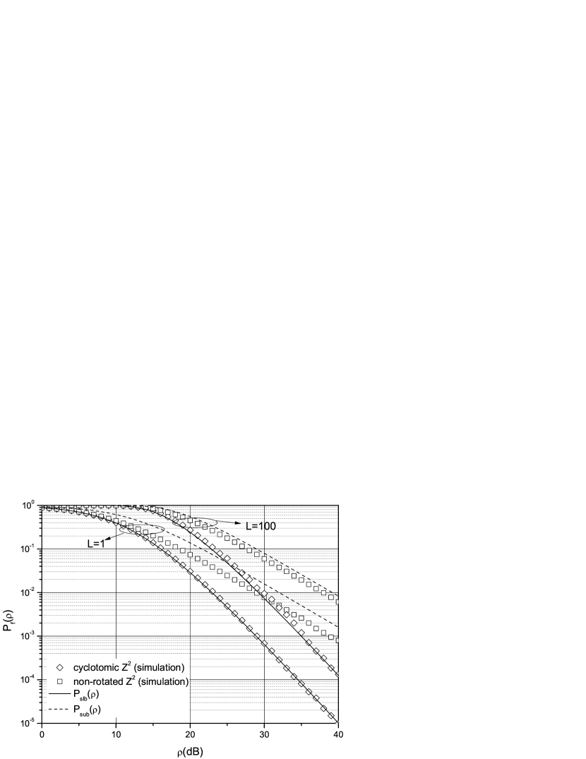
Figure 1: Frame Error Probability, SLB and SUB for the $\mathbb{Z}^{2}$ infinite lattice constellation, for $m=1$ and $L=1,100$.

Fig. 1 depicts the accuracy and tightness of the SLB and the SUB along with the frame error probability of $\mathbb{Z}^{2}$ infinite lattice constellations, for various values of frame lengths. Specifically, the analytical results obtained from (38) and (39) are plotted in conjunction with simulation results for the frame error probability of the cyclotomic rotation of the $\mathbb{Z}^{2}$ infinite lattice constellation and the non rotated lattice, when $m=1$ and $L=1,100$. As it is clearly illustrated, the numerical results obtained from the analytical expressions act as lower and upper bounds in all cases examined. In particular, as the known SLB is observed to be very close to the performance of optimally rotated lattices, the SUB seems to be less tight but still very close to the non-rotated case. Moreover, as the frame length $L$ increases, it is evident that the proposed SUB becomes even tighter. It can be observed that the diversity order, i.e. the asymptotic slope of the frame error probability, is independent of the frame length, for both the lattices under investigation and their SLB and SUB.

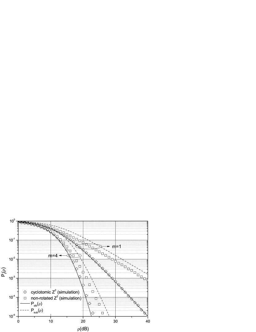
Figure 2: Frame Error Probability, SLB and SUB for the $\mathbb{Z}^{2}$ infinite lattice constellation, for $m=1,4$ and $L=1$.

Fig. 2 demonstrates the results for SLB and SUB along with the simulated performance of the $\mathbb{Z}^{2}$ infinite lattice constellations for various values of the m parameter. It is evident that both the SLB and the SUB act as tight bounds, irrespective of $m$. Moreover, the effects of the $m$-parameter on the diversity order of both lattices under investigation and their bounds, are clearly depicted.

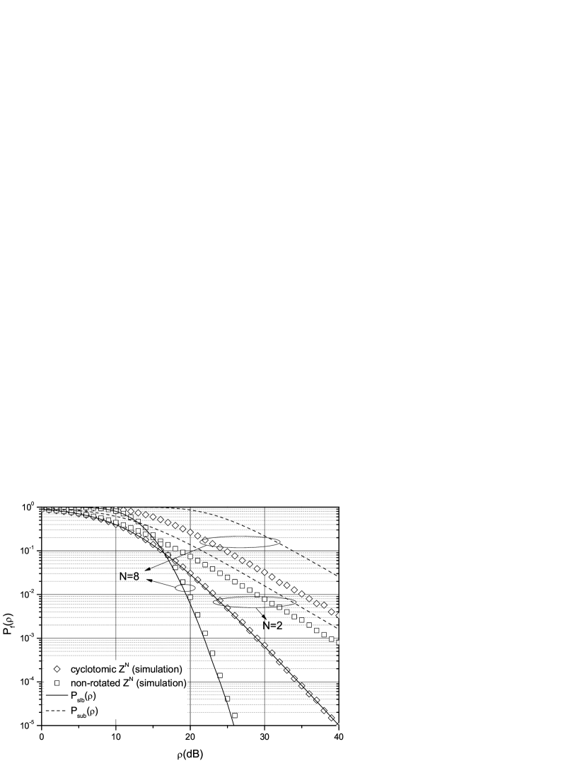
Figure 3: Frame Error Probability, SLB and SUB for the $\mathbb{Z}^{N}$ infinite lattice constellation, for $m=1$ $L=1$ and $N=2,8$.

Fig. 3 illustrates the effect of the dimension order on the frame error probability of the $\mathbb{Z}^{N}$ infinite lattice constellations and the corresponding SLB and SUB. In particular, we consider $m=1$, $L=1$ and $N=2,8$. It is obvious that the SLB and SUB act as bounds irrespective of the dimension $N$, while the SUB is tighter for small dimension. The SUB has similar diversity order with the non rotated lattices and the SLB has similar diversity order with the optimally rotated lattices which achieve full diversity.

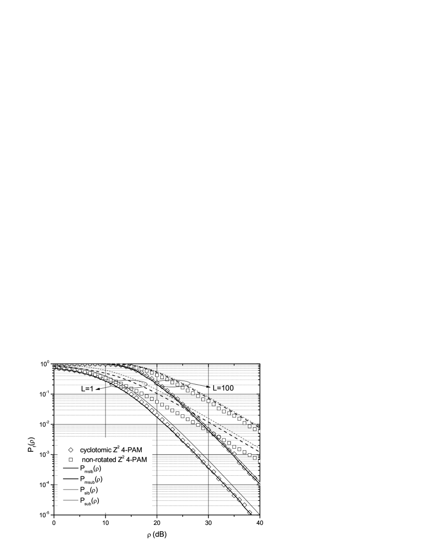
Figure 4: Frame Error Probability, MSLB, MSUB, SLB and SUB for the $\mathbb{Z}^{2}$ $4$-PAM constellation, for $m=1$ and $L=1,100$.

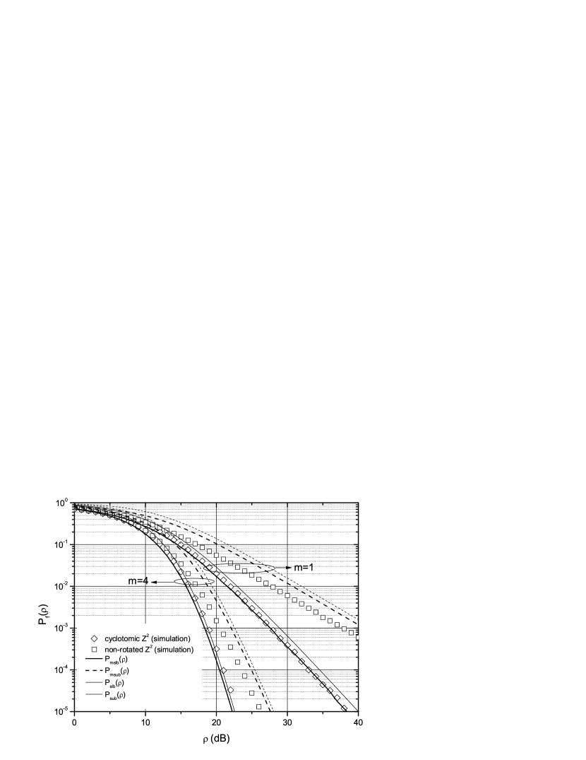
Figure 5: Frame Error Probability, MSLB, MSUB, SLB and SUB for the $\mathbb{Z}^{2}$ $4$-PAM constellation, for $m=1,4$ and $L=1$.

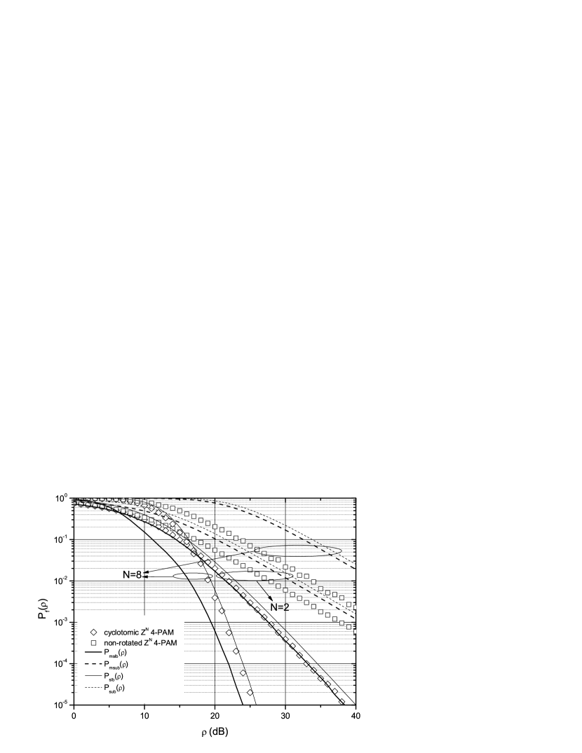
Figure 6: Frame Error Probability, MSLB, MSUB, SLB and SUB for the $\mathbb{Z}^{N}$ $4$-PAM constellation, for $m=1$, $L=1$ and $N=2,8$.

Figs. 4, 5 and 6 illustrate the performance obtained via Monte-Carlo simulation of finite $\mathbb{Z}^{N}$ $4$-PAM lattice constellations for various values of block length $L$, parameter $m$ and dimension $N$ respectively. These figures correspond to the cases of Figs. 1, 2 and 3 for infinite lattice constellations. The MSLB and MSUB are illustrated for each case, in addition to the corresponding SLB and SUB for the infinite lattices as a reference. One can observe that the behavior of the MSLB and MSUB with respect to the performance of a finite constellation is extremely similar to that of the SLB and SUB with respect to the performance of an infinite constellation. However, it is clearly illustrated that the MSLB and MSUB bounds are more appropriate for a finite lattice constellations than the SLB and SUB. Specifically, as shown in Fig. 4, the SLB does not act as a bound for finite constellations, whereas the MSLB is always a lower bound and it is tighter to the simulated performance of the optimally rotated lattices than the SLB. Similarly, the MSUB is tighter than the SUB to the simulated performance of the non-rotated lattices. For higher values of the $m$ parameter, while the SLB is not a lower bound for low SNR values, the MSLB remains below the simulated performance of the optimally rotated lattices for all values of SNR. In Fig. 6, the MSLB for higher dimensions is rather loose for low SNR values, but becomes tighter as the SNR increases. However, it is the only reliable bound, since the SLB is above the simulated performance of the optimally rotated lattice for all SNR values. Both expressions can be used, the MSLB as a reliable lower bound and the SLB as a good approximation of the actual performance. Finally for the MSUB, it is tighter than the SUB in all cases.

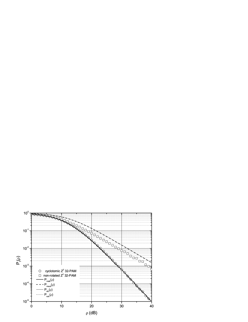
Figure 7: Frame Error Probability, MSLB, MSUB, SLB and SUB for the $\mathbb{Z}^{2}$ $32$-PAM constellation, for $m=1$ and $L=1$.

The MSLB and MSUB also take into account the number $K$ of points along the direction of each basis vector of the constellations. In Fig. 7, constellations of larger $K$ are depicted, that is the optimally rotated and the non-rotated $\mathbb{Z}^{2}$ $32$-PAM. It is again evident that the MSLB is an extremely tight lower bound, regardless of the rank of the constellation. Moreover, the MSUB is also accurate and tight, illustrating that the tightness of the bounds is not noticeably affected by the rank of the constellations. Finally, it can be deduced that as the parameter $K$ increases, the MSLB and MSUB tend to coincide with the SLB and the SUB respectively. This is expected, since the number of inner points on the constellation, which are approximated in the same way in the two pairs of bounds, is much larger than the number of outer points.

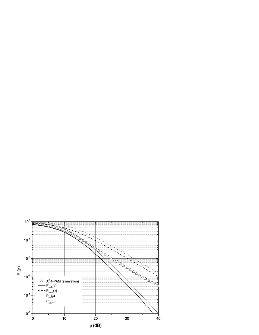
Figure 8: Frame Error Probability, MSLB, MSUB, SLB and SUB for the $\mathbb{A}^{2}$ $4$-PAM constellation, for $m=1$ and $L=1$.

Finally, in Fig. 8, the performance of a constellation carved from a lattice with different structure is depicted, together with the numerical results for the corresponding MSLB and MSUB. Specifically, the $\mathbb{A}^{2}$ $4$-PAM constellation is illustrated, which is the best known packing lattice in two dimensions [21], with generator matrix

$$M=\left[\begin{array}[]{cc}\sqrt{\frac{2}{\sqrt{3}}}&\sqrt{\frac{1}{2\sqrt{3}}}\\ 0&\sqrt{\frac{3}{2\sqrt{3}}}\end{array}\right].$$ (42)

The MSLB and MSUB again bound the performance of this lattice constellation, while the SLB is not a reliable bound and the SUB is looser than the MSUB. Moreover, the figure suggests that the simulated rotation of the constellation is not optimal with respect to the diversity gain and the maximization of the minimum product distance. This is an important result, not only for this constellation but also for other signal sets with random rotation, because the bounds act as indication of the optimality of a designed constellation.

V Conclusions

We have studied the error performance of multidimensional lattice constellations in block fading channels. We first presented analytical expressions for the exact FEP of both infinite and finite signal sets carved from lattices, in the presence of Nakagami-m block fading. These expressions were then bounded by the well known SLB and the novel SUB proposed for the infinite lattice constellations, as well as by the proposed MSLB and MSUB for finite lattice constellations of arbitrary structure, rank and dimension. Then, analytical closed form expressions were derived for the SUB and SLB in lattices with even dimensions, whereas the MSLB and MSUB were given in closed form for constellations of even dimensions and for transmission in fading channels with single-symbol block length. The proposed analytical framework sets the performance limits of such signal sets and it can be an efficient tool for their analysis and design.

Appendix A Proof of Theorem 1

The volume of $\mathcal{V}_{\mathcal{S}_{k,p}}(\mathbf{H})$ in (17) is the same as the volume of the corresponding fundamental parallelotope of a faded sublattice, for which holds [1, Eq. (41)]

$$\mathrm{vol}_{k}(\mathcal{V}_{\mathcal{S}_{k,p}}(\mathbf{H}))\leq\prod_{i:\mathbf{v}_{i}\in\mathcal{S}_{k,p}}\|\mathbf{Hv}_{i}\|\leq\prod_{i:\mathbf{v}_{i}\in\mathcal{S}_{k,p}}\|\mathbf{v}_{i}\|\max\limits_{j=1,\ldots,N}h_{j},$$ (43)

where the first equality is true only when the vectors of $\mathcal{S}_{k,p}$ distorted by fading are orthogonal. The second equality holds only if all fading coefficients $h_{j}$ are equal to $\max\limits_{j=1,\ldots,N}h_{j}$. Moreover, the inequalities in (43) imply that the volume of a faded Voronoi cell of a sublattice $\mathcal{S}_{k,p}$ will always be at most equal to the volume of a rectangular parallelotope, with edges of norms equal to those of the vectors in $\mathcal{S}_{k,p}$, multiplied by the largest fading coefficient. Using (43) yields to

$$\sum\limits_{p=1}^{\binom{N}{k}}\mathrm{vol}_{k}(\mathcal{V}_{\mathcal{S}_{k,p}}(\mathbf{H}))\leq\sum\limits_{p=1}^{\binom{N}{k}}\prod_{i:\mathbf{v}_{i}\in\mathcal{S}_{k,p}}\|\mathbf{v}_{i}\|\max\limits_{j=1,\ldots,N}h_{j},$$ (44)

which can be written as

$$\sum\limits_{p=1}^{\binom{N}{k}}\mathrm{vol}_{k}(\mathcal{V}_{\mathcal{S}_{k,p}}(\mathbf{H}))\leq\left(\max\limits_{j=1,\ldots,N}h_{j}\right)^{k}\sum\limits_{\begin{subarray}{c}b_{1}+b_{2}+\ldots+b_{N}=k\\ b_{1},b_{2},\ldots,b_{N}\in\{0,1\}\end{subarray}}\|\mathbf{v}_{1}\|^{b_{1}}\|\mathbf{v}_{2}\|^{b_{2}}\cdots\|\mathbf{v}_{N}\|^{b_{N}}.$$ (45)

Using Maclaurin’s Inequality [20, p.52], for $a_{1},a_{2},\ldots,a_{N}\in\mathbb{R}$ and $0<k<N$,

$$\varrho_{N}^{\frac{1}{N}}\leq\varrho_{k}^{\frac{1}{k}}\leq\varrho_{1},$$ (46)

where

$$\varrho_{k}=\frac{\sum\limits_{\begin{subarray}{c}b_{1}+b_{2}+\ldots+b_{N}=k\\ b_{1},b_{2},\ldots,b_{N}\in\{0,1\}\end{subarray}}a_{1}^{b_{1}}a_{2}^{b_{2}}\cdots a_{N}^{b_{N}}}{\binom{N}{k}}.$$ (47)

If we set $a_{i}=\|\mathbf{v}_{i}\|$, $i=1,2,\ldots,N$, then $\varrho_{1}=W$ and from (46) and (47)

$$\sum\limits_{\begin{subarray}{c}b_{1}+b_{2}+\ldots+b_{N}=k\\ b_{1},b_{2},\ldots,b_{N}\in\{0,1\}\end{subarray}}\|\mathbf{v}_{1}\|^{b_{1}}\|\mathbf{v}_{2}\|^{b_{2}}\cdots\|\mathbf{v}_{N}\|^{b_{N}}\leq\binom{N}{k}W^{k}.$$ (48)

From (45) and (48), for $0<k<N$, we have

$$\sum\limits_{p=1}^{\binom{N}{k}}\mathrm{vol}_{k}(\mathcal{V}_{\mathcal{S}_{k,p}}(\mathbf{H}))\leq\left(\max\limits_{j=1,\ldots,N}h_{j}\right)^{k}\binom{N}{k}W^{k}.$$ (49)

For the spheres $\mathcal{B}_{\mathcal{S}_{k,p}}(\mathbf{H})$ with $\mathrm{vol}_{k}(\mathcal{B}_{\mathcal{S}_{k,p}}(\mathbf{H}))=\mathrm{vol}_{k}(\mathcal{V}_{\mathcal{S}_{k,p}}(\mathbf{H}))$, holds that

$$\sum\limits_{p=1}^{\binom{N}{k}}J_{k,p}(\mathbf{H})\leq\sum\limits_{p=1}^{\binom{N}{k}}\int_{\mathcal{B}_{\mathcal{S}_{k,p}}(\mathbf{H})}p(\mathbf{z})\mathrm{d}\mathbf{z}=\sum\limits_{p=1}^{\binom{N}{k}}\left(1-\frac{\Gamma\left(\frac{k}{2},\frac{R_{\mathcal{S}_{k,p}}^{2}(\mathbf{H})}{2}\rho\right)}{\Gamma\left(\frac{k}{2}\right)}\right),$$ (50)

where $R_{\mathcal{S}_{k,p}}(\mathbf{H})$ is the radius of $\mathcal{B}_{\mathcal{S}_{k,p}}(\mathbf{H})$. From (49), and using that $\mathrm{vol}_{k}\left(\mathcal{B}_{\mathcal{S}_{k,p}}(\mathbf{H})\right)=\frac{\pi^{\frac{k}{2}}R_{\mathcal{S}_{k,p}}^{k}(\mathbf{H})}{\Gamma\left(\frac{k}{2}+1\right)}$

$$\sum\limits_{p=1}^{\binom{N}{k}}\frac{\pi^{\frac{k}{2}}R_{\mathcal{S}_{k,p}}^{k}(\mathbf{H})}{\Gamma\left(\frac{k}{2}+1\right)}\leq\left(\max\limits_{j=1,\ldots,N}h_{j}\right)^{k}\binom{N}{k}W^{k}.$$ (51)

Furthermore, by taking into account (21) for the case when $0<k<N$,

$$\sum\limits_{m=1}^{\binom{N}{k}}R_{\mathcal{S}_{k,m}}^{k}(\mathbf{H})\leq\binom{N}{k}R_{k}^{k}(\mathbf{H}).$$ (52)

As proved in [1], the function $f(x;a,b)=\Gamma\left(a,bx^{1/a}\right)$ is convex in $(0,\infty)$, thus from Jensen’s Inequality for convex functions [20] holds that

$$\sum_{i=1}^{M}{\Gamma\left(a,b{x_{i}}^{1/a}\right)}\geq M\Gamma\left(a,b\left(\sum_{i=1}^{L}{x_{i}}/L\right)^{1/a}\right).$$ (53)

For $a=\frac{k}{2}$ , $b=\frac{\rho}{2}$, $M=\binom{N}{k}$ and $x_{i}={R^{k}_{\mathcal{S}_{k,p}}}$ we get

$$\sum_{p=1}^{\binom{N}{k}}{\Gamma\left(\frac{k}{2},\frac{\rho}{2}R^{2}_{\mathcal{S}_{k,p}}(\mathbf{H})\right)}\geq\binom{N}{k}\Gamma\left(\frac{k}{2},\frac{\rho}{2}\left(\frac{\sum\limits_{m=1}^{\binom{N}{k}}R^{k}_{\mathcal{S}_{k,p}}(\mathbf{H})}{\binom{N}{k}}\right)^{\frac{2}{k}}\right).$$ (54)

From (52) and since $f(x;a,b)=\Gamma\left(a,bx^{1/a}\right)$ is a monotonically decreasing function with respect to $x$,

$$\Gamma\left(\frac{k}{2},\frac{\rho}{2}\left(\frac{\sum\limits_{p=1}^{\binom{N}{k}}R^{k}_{\mathcal{S}_{k,p}}(\mathbf{H})}{\binom{N}{k}}\right)^{\frac{2}{k}}\right)\geq\Gamma\left(\frac{k}{2},\frac{\rho}{2}R^{2}_{k}(\mathbf{H})\right).$$ (55)

Using (54) and (55), for $0<k<N$

$$\sum_{p=1}^{\binom{N}{k}}{\Gamma\left(\frac{k}{2},\frac{\rho}{2}R^{2}_{\mathcal{S}_{k,p}}(\mathbf{H})\right)}\geq\binom{N}{k}\Gamma\left(\frac{k}{2},\frac{\rho}{2}R^{2}_{k}(\mathbf{H})\right),$$ (56)

or equivalently

$$\sum_{p=1}^{\binom{N}{k}}\left(1-\frac{\Gamma\left(\frac{k}{2},\frac{\rho}{2}R^{2}_{\mathcal{S}_{k,p}}(\mathbf{H})\right)}{\Gamma\left(\frac{k}{2}\right)}\right)\leq\binom{N}{k}\left(1-\frac{\Gamma\left(\frac{k}{2},\frac{\rho}{2}R^{2}_{k}(\mathbf{H})\right)}{\Gamma\left(\frac{k}{2}\right)}\right).$$ (57)

Taking into account (50) and (57) for some $k$, $0<k<N$, it yields

$$\sum\limits_{p=1}^{\binom{N}{k}}J_{k,p}\leq\binom{N}{k}\left(1-\frac{\Gamma\left(\frac{k}{2},\frac{\rho}{2}R^{2}_{k}(\mathbf{H})\right)}{\Gamma\left(\frac{k}{2}\right)}\right)=\binom{N}{k}I_{k}(\mathbf{H}).$$ (58)

For the case when $k=0$, $p=1$ and it holds that $J_{0}(\mathbf{H})=I_{0}(\mathbf{H})=1$. For $k=N$, it is also $p=1$ and from (21), since $\mathrm{vol}_{N}\left(\mathcal{V}_{\mathcal{S}_{N}}(\mathbf{H})\right)=\frac{\pi^{\frac{N}{2}}R_{N}^{k}(\mathbf{H})}{\Gamma\left(\frac{N}{2}+1\right)}$

$$J_{N}(\mathbf{H})\leq\left(1-\frac{\Gamma\left(\frac{N}{2},\frac{\rho}{2}R^{2}_{N}(\mathbf{H})\right)}{\Gamma\left(\frac{N}{2}\right)}\right)=I_{N}(\mathbf{H}).$$ (59)

Combining (58) and (59), multiplying by $\left(K-1\right)^{k}$ and summing for all $k$, it results to

$$\sum\limits_{k=0}^{N}\left(K-1\right)^{k}\sum\limits_{p=1}^{\binom{N}{k}}J_{k,p}(\mathbf{H})\leq\sum\limits_{k=0}^{N}\left(K-1\right)^{k}\binom{N}{k}I_{k}(\mathbf{H}).$$ (60)

Finally, using (19), (25) and (60)

$$P_{mslb}(\rho)\leq P_{f,K-PAM}(\rho)$$ (61)

and this concludes the proof.

Appendix B Proof of Theorem 2

The proof starts by approximating the decision region of the faded lattice, $\mathcal{V}_{\mathcal{S}_{N}}\left(\mathbf{H}\right)$, with a sphere, whose radius is equal with the packing radius of the lattice [7, 21], i.e., the minimum Euclidean distance between the origin of the lattice and the facets of $\mathcal{V}_{\mathcal{S}_{N}}\left(\mathbf{H}\right)$. If $q$ is the number of neighboring symbols around a point of the unfaded lattice, and $\mathbf{d_{i}}$ with $i=1,...,q$, is the vector from the point investigated to the $i$-th neighboring one, the sphere packing radius for a given channel realization $\mathbf{H}$ becomes equal to the minimum Euclidean distance on the faded lattice, namely

$$d_{min,\mathcal{S}_{N}}(\mathbf{H})=\min\limits_{i=1,\ldots,q}\frac{\|\mathbf{Hd_{i}}\|}{2}=\min\limits_{i=1,\ldots,q}\frac{\sqrt{\sum\limits_{j=1}^{N}h_{j}^{2}d_{ij}^{2}}}{2}$$ (62)

However for any $\mathbf{d_{i}}$ holds that

$$\sqrt{\sum\limits_{j=1}^{N}h_{j}^{2}d_{ij}^{2}}\geq\|\mathbf{d_{i}}\|\min_{j=1,\ldots,N}h_{j}.$$ (63)

Thus, we can conclude that

$$\min\limits_{i=1,\ldots,q}\left(\frac{\sqrt{\sum\limits_{j=1}^{N}h_{j}^{2}d_{ij}^{2}}}{2}\right)\geq\min\limits_{i=1,\ldots,q}\frac{\|\mathbf{d_{i}}\|\min\limits_{j=1,\ldots,N}\left(h_{j}\right)}{2},$$ (64)

or equivalently

$$d_{min,\mathcal{S}_{N}}(\mathbf{H})=\min\limits_{i=1,\ldots,q}\frac{\sqrt{\sum\limits_{j=1}^{N}h_{j}^{2}d_{ij}^{2}}}{2}\geq\frac{d_{\min}}{2}\min\limits_{j=1...,N}h_{j},$$ (65)

where $d_{min}=\min\limits_{i=1,\ldots,q}\|\mathbf{d_{i}}\|$ is the minimum Euclidean distance between adjacent points on the unfaded infinite lattice constellation. Therefore, the packing radius of the faded lattice can be lower bounded by (26), which yields an upper bound on the frame error probability, $P_{sub}(\rho)$, given in (28). This concludes the proof.

Appendix C Proof of Theorem 3

For a faded sublattice defined by $\mathcal{S}_{k,p}$, similarly to Appendix B, the minimum Euclidean distance $d_{min,\mathcal{S}_{k,p}}(\mathbf{H})$ between adjacent points can be lower bounded by

$$d_{min,\mathcal{S}_{k,p}}(\mathbf{H})\geq\frac{d_{min,\mathcal{S}_{k,p}}}{2}\min\limits_{j=1...,N}h_{j},$$ (66)

where $d_{min,\mathcal{S}_{k,p}}$ is the minimum Euclidean distance between adjacent points on the unfaded sublattice defined by $\mathcal{S}_{k,p}$. Since $\mathcal{S}_{k,p}\subseteq\mathcal{S}_{N}$, it holds that

$$d_{min,\mathcal{S}_{k,p}}\geq d_{min}$$ (67)

and consequently

$$d_{min,\mathcal{S}_{k,p}}(\mathbf{H})\geq\frac{d_{min}}{2}\min\limits_{j=1...,N}h_{j}.$$ (68)

Thus, the packing radius of every faded sublattice defined by $\mathcal{S}_{k,p}$ can be lower bounded by (26) and the integrals in (27) are lower bounds to the integrals on the faded Voronoi cells $\mathcal{V}_{\mathcal{S}_{k,p}}(\mathbf{H})$, making the expression in (29) an upper bound of the FEP of finite lattice constellations. This concludes the proof.

Appendix D Closed Form for the Function $A(\rho,N;k,L)$

The following function

$$A(\rho,N;k,L)=\mathbb{E}\left[\left(1-\frac{\Gamma\left(\frac{k}{2},\frac{\mathcal{R}^{2}\left(\mathbf{H}\right)}{2}\rho\right)}{\Gamma\left(\frac{k}{2}\right)}\right)^{L}\right],$$ (69)

can be written as [17, Eq. (1.111)]

$$A(\rho,N;k,L)=\sum\limits_{q=0}^{L}\binom{L}{q}\frac{\left(-1\right)^{q}}{\left(\Gamma\left(\frac{k}{2}\right)\right)^{q}}\mathbb{E}\left[\left(\Gamma\left(\frac{k}{2},\frac{\mathcal{R}^{2}\left(\mathbf{H}\right)}{2}\rho\right)\right)^{q}\right].$$ (70)

Using an alternative representation for the upper incomplete Gamma function [17, Eq. (8.352/2)] and applying the multinomial theorem, we obtain

$$\left[\Gamma\left(\frac{k}{2},\frac{\mathcal{R}^{2}\left(\mathbf{H}\right)}{2}\rho\right)\right]^{q}=\exp\left(-\frac{q\mathcal{R}^{2}\left(\mathbf{H}\right)}{2}\rho\right)\left(\Gamma\left(\frac{k}{2}\right)\right)^{q}\Gamma\left(q+1\right)\times\sum\limits_{\begin{subarray}{c}n_{0},...,n_{\frac{k}{2}-1}=0\\ n_{0}+...+n_{\frac{k}{2}-1}=q\end{subarray}}^{q}\frac{\left(\frac{\mathcal{R}^{2}\left(\mathbf{H}\right)}{2}\rho\right)^{\mathcal{Z}}}{\Psi},$$ (71)

where $\mathcal{Z}=\sum\limits_{i=0}^{\frac{k}{2}-1}in_{i}$ and $\Psi=\prod\limits_{i=0}^{\frac{k}{2}-1}\left(\left(i!\right)^{n_{i}}\Gamma\left(n_{i}+1\right)\right)$.

Hence, (70) can be rewritten as

$$A(\rho,N;k,L)=\sum\limits_{q=0}^{L}\sum_{\begin{subarray}{c}n_{0},...,n_{\frac{k}{2}-1}=0\\ n_{0}+...+n_{\frac{k}{2}-1}=q\end{subarray}}^{q}\frac{L!}{\left(L-q\right)!}\frac{\left(-1\right)^{q}\rho^{\mathcal{Z}}}{\Psi}\,\mathcal{E}_{1},$$ (72)

where

$$\mathcal{E}_{1}=\mathbb{E}\left[\left(\frac{\mathcal{R}^{2}\left(\mathbf{H}\right)}{2}\right)^{\mathcal{Z}}\exp\left(-\frac{q\mathcal{R}^{2}\left(\mathbf{H}\right)}{2}\rho\right)\right].$$ (73)

Taking into consideration that the cdf of $\gamma_{\min}=\min\limits_{i=1,\ldots,N}\gamma_{i}$ is given by

$$P_{\gamma_{\min}}\left(x\right)=1-\left(\frac{\Gamma\left(m,mx\right)}{\Gamma\left(m\right)}\right)^{N},$$ (74)

and after employing [17, Eq. (8.356.4)], the pdf of $\mathcal{R}^{2}\left(\mathbf{H}\right)$ can be straightforwardly derived, according to (26), as

$$p_{\mathcal{R}^{2}}\left(x\right)=\frac{\left[\Gamma\left(m,\frac{4m}{d_{\min}^{2}}x\right)\right]^{N-1}x^{m-1}\exp\left(-\frac{4m}{d_{\min}^{2}}x\right)}{\left(\frac{d_{\min}^{2}}{4}\right)^{m}m^{-m}\left[\Gamma\left(m\right)\right]^{N}N^{-1}},.$$ (75)

Equivalently, using (71), (75) can be written as

$$p_{\mathcal{R}^{2}}\left(x\right)=\frac{N\exp\left(-\frac{4mN}{d_{\min}^{2}}x\right)}{\left(\frac{d_{\min}^{2}}{4m}\right)^{-1}\frac{\Gamma\left(m\right)}{\Gamma\left(N\right)}}\sum_{\begin{subarray}{c}t_{0},...,t_{m-1}=0\\ t_{0}+...+t_{m-1}=N-1\end{subarray}}^{N-1}\frac{\left(\frac{4m}{d_{\min}^{2}}x\right)^{\mathcal{Y}+m-1}}{\Xi}.$$ (76)

where $\mathcal{Y}=\sum\limits_{j=0}^{m-1}jt_{j}$ and $\Xi=\prod\limits_{j=0}^{m-1}\left(\left(j!\right)^{t_{j}}\Gamma\left(t_{j}+1\right)\right)$.

Hence, for the expectation in (73), denoted as $\mathcal{E}_{1}$, when $q=0$, it holds that $\mathcal{Z}=\sum\limits_{i=0}^{\frac{k}{2}-1}in_{i}=0$ and thus $\mathcal{E}_{1}=1$, while for $q>0$, $\mathcal{E}$ can be can be analytically evaluated as [17, Eq. (3.326.2)]

$$\mathcal{E}_{1}=\frac{Nm^{m}}{\Gamma\left(m\right)}\sum_{\begin{subarray}{c}t_{0},...,t_{m-1}=0\\ t_{0}+...+t_{m-1}=N-1\end{subarray}}^{N-1}\frac{m^{\mathcal{Y}}\left(\frac{d_{\min}^{2}}{8}\right)^{\mathcal{Z}}\Gamma\left(\mathcal{Y}+m+\mathcal{Z}\right)}{\Xi\left(mN+\frac{q\rho d_{\min}^{2}}{8}\right)^{\mathcal{Y}+m+\mathcal{Z}}}$$ (77)

Finally, by combining (72) with (77) and taking into account the case for $q=0$, it yields (31) and this concludes the proof.

Appendix E Closed Form for the Function $B(\rho,N;k)$

The function

$$\begin{array}[]{cc}B(\rho,N;k)=\mathbb{E}\left[1-\frac{\Gamma\left(\frac{k}{2},\frac{R_{k}^{2}\left(\mathbf{H}\right)}{2}\rho\right)}{\Gamma\left(\frac{k}{2}\right)}\right],&0<k<N,\end{array}$$ (78)

can be written, using (21), as

$$B(\rho,N;k)=1-\frac{1}{\Gamma\left(\frac{k}{2}\right)}\mathbb{E}\left[\Gamma\left(\frac{k}{2},\frac{\rho\Gamma\left(\frac{k}{2}+1\right)^{\frac{2}{k}}W^{2}}{2\pi}\max_{i=1,...,N}\left(\gamma_{i}\right)\right)\right],$$ (79)

or if we set $b=\max\limits_{i=1,...,N}\gamma_{i}$, then

$$B(\rho,N;k)=1-\frac{1}{\Gamma\left(\frac{k}{2}\right)}\int_{0}^{\infty}\Gamma\left(\frac{k}{2},\frac{\rho\Gamma\left(\frac{k}{2}+1\right)^{\frac{2}{k}}W^{2}}{2\pi}x\right)f_{b}\left(x\right)dx.$$ (80)

The cdf of $b$ is

$$F_{b}\left(x\right)=\left(1-\frac{\Gamma\left(m,mx\right)}{\Gamma\left(m\right)}\right)^{N}=\sum\limits_{q=0}^{N}\binom{N}{q}\frac{\Gamma\left(m,mx\right)^{q}}{\Gamma\left(m\right)^{q}}.$$ (81)

Now, as in (71), (81) can be rewritten as

$$F_{b}\left(x\right)=\sum\limits_{q=0}^{N}\binom{N}{q}\exp\left(-qmx\right)\Gamma\left(q+1\right)\sum_{\begin{subarray}{c}n_{0},n_{1},...,n_{m-1}=0\\ n_{0}+n_{1}+...+n_{m-1}=q\end{subarray}}^{q}x^{\mathcal{X}}\Upsilon,$$ (82)

where $\mathcal{X}=\sum\limits_{i=0}^{m-1}in_{i}$ and $\Upsilon=\prod\limits_{i=0}^{m-1}\frac{\left(\frac{m^{i}}{i!}\right)^{n_{i}}}{\Gamma\left(n_{i}+1\right)}$.

The pdf of $b$ is obtained by taking the derivative of (82) as

$$f_{b}\left(x\right)=\sum\limits_{q=0}^{N}\binom{N}{q}\exp\left(-qmx\right)\Gamma\left(q+1\right)\sum\limits_{\begin{subarray}{c}n_{0},n_{1},...,n_{m-1}=0\\ n_{0}+n_{1}+...+n_{m-1}=q\end{subarray}}^{q}x^{\left[\mathcal{X}-1\right]}\left(-qmx+\mathcal{X}\right)\Upsilon.$$ (83)

Hence, (80) becomes equivalent with

$$\begin{array}[]{ll}B(\rho,N;k)=1-\sum\limits_{q=0}^{N}\frac{\binom{N}{q}\Gamma\left(q+1\right)}{\Gamma\left(\frac{k}{2}\right)}&\times\left\{\sum\limits_{\begin{subarray}{c}n_{0},n_{1},...,n_{m-1}=1\\ n_{0}+n_{1}+...+n_{m-1}=q\\ \sum\limits_{i=0}^{m-1}in_{i}\neq 0\end{subarray}}^{q}\mathcal{X}\Upsilon f\left(\mathcal{X},\frac{\rho\Gamma\left(\frac{k}{2}+1\right)^{\frac{2}{k}}W^{2}}{2\pi},qm,\frac{k}{2}\right)\right.\\ &\left.-\sum\limits_{\begin{subarray}{c}n_{0},n_{1},...,n_{m-1}=1\\ n_{0}+n_{1}+...+n_{m-1}=q\end{subarray}}^{q}qm\Upsilon f\left(\mathcal{X}+1,\frac{\rho\Gamma\left(\frac{k}{2}+1\right)^{\frac{2}{k}}W^{2}}{2\pi},qm,\frac{k}{2}\right)\right\},\end{array}$$ (84)

where

$$f\left(\alpha,\beta,p,\nu\right)=\int_{0}^{\infty}x^{\alpha-1}\Gamma\left(\nu,\beta x\right)\exp\left(-px\right)dx.$$ (85)

Using [22, Eq. (2.10.3.2)], (84) can be reduced to (33) with $g\left(\alpha,\beta,p,\nu\right)$ as defined in (34), and this concludes the proof.

Appendix F Closed Form for the Function $C(\rho,N;L)$

The function

$$C(\rho,N;L)=\mathbb{E}\left[\left(1-\frac{\Gamma\left(\frac{N}{2},\frac{R_{N}^{2}\left(\mathbf{H}\right)}{2}\rho\right)}{\Gamma\left(\frac{N}{2}\right)}\right)^{L}\right],$$ (86)

can be written, following a similar analysis as in Appendix D, as

$$C(\rho,N;L)=\sum\limits_{q=0}^{L}\sum_{\begin{subarray}{c}n_{0},...,n_{\frac{N}{2}-1}=0\\ n_{0}+...+n_{\frac{N}{2}-1}=q\end{subarray}}^{q}\frac{\frac{L!}{\left(L-q\right)!}\left(-1\right)^{q}\left(\frac{1}{2}\rho\right)^{\mathcal{Q}}}{\Phi}\,\mathcal{E}_{2},$$ (87)

where $\mathcal{Q}=\sum\limits_{i=0}^{\frac{N}{2}-1}in_{i}$, $\Phi=\prod\limits_{i=0}^{\frac{N}{2}-1}\left(\left(i!\right)^{n_{i}}\Gamma\left(n_{i}+1\right)\right)$ and

$$\mathcal{E}_{2}\mathcal{=}\mathbb{E}\left[\left(R_{N}^{2}\left(\mathbf{H}\right)\right)^{\mathcal{Q}}\exp\left(-\frac{qR_{N}^{2}\left(\mathbf{H}\right)}{2}\rho\right)\right].$$ (88)

Using [23, Eq. (5)] and after a variable transformation, the pdf of $R_{N}^{2}\left(\mathbf{H}\right)$ can be straightforwardly obtained for Nakagami fading model as

$$p_{R_{N}^{2}}\left(x\right)=\frac{Nx^{-1}}{\left(\Gamma\left(m\right)\right)^{N}}G_{0,N}^{N,0}\left[\left(\frac{\pi xm}{\left(\Gamma\left(\frac{N}{2}+1\right)\right)^{\frac{2}{N}}}\right)^{N}\left|\begin{array}[]{c}-\\ m,...,m\\ \end{array}\right.\right].$$ (89)

Hence, for the expectation in (88), denoted as $\mathcal{E}_{2}$, when $q=0$ it is $\mathcal{E}_{2}=1$, whereas for $q\neq 0$, it can be analytically evaluated, by expressing its integrand $\exp\left(\cdot\right)$ in terms of Meijer’s G-functions according to [24, Eq. (8.4.3.1)] and using [24, Eq. (2.24.1.1)], as

$$\mathcal{E}_{2}=\frac{\sqrt{N}\left(\frac{2N}{q\rho}\right)^{\mathcal{Q}}}{\left(\Gamma\left(m\right)\right)^{N}\left(2\pi\right)^{\frac{N-1}{2}}}G_{N,N}^{N,N}\left[\frac{\left(\frac{2\pi mN}{q\rho}\right)^{N}}{\left(\Gamma\left(\frac{N}{2}+1\right)\right)^{2}}\left|\begin{array}[]{c}\frac{1-\mathcal{Q}}{N},...,\frac{N-\mathcal{Q}}{N}\\ m,...,m\\ \end{array}\right.\right].$$ (90)

By combining (90) with (87), and taking into account the special case for $q=0$, (87) can be written as in (36) and this concludes the proof.

References

• [1] K. N. Pappi, N. D. Chatzidiamantis and G. K. Karagiannidis, โ€œError Performance of Multidimensional Lattice Constellations - Part I: A Parallelotope Geometry Based Approach for the AWGN Channelโ€, submitted to IEEE Trans. Commun.
• [2] J. Boutros and E. Viterbo, โ€œSignal Space Diversity: A power- and bandwidth-efficient diversity technique for the Rayleigh fading channelโ€, IEEE Trans. Inf. Theory, vol. 44, no. 4, p. 1453โ€“1467, Jul. 1998.
• [3] J. Boutros, E. Viterbo, C. Rastello, and J. C. Belfiore, โ€œGood lattice constellations for both Rayleigh fading and Gaussian channelsโ€, IEEE Trans. Inf. Theory, vol. 42, no. 2 pp. 502โ€“518, Mar. 1996.
• [4] X. Giraud, E. Boutillon, and J. C. Belfiore, โ€œAlgebraic tools to build modulation schemes for fading channelsโ€, IEEE Trans. Inf. Theory, vol. 43, no. 3, pp. 938-952, May 1997.
• [5] E. Bayer-Fluckiger, F. Oggier, and E. Viterbo, โ€œNew algebraic constructions of rotated Zn-lattice constellations for the Rayleigh fading channel,โ€ย IEEE Trans. Inf. Theory, vol. 50, no. 4, pp. 702โ€“714, Apr. 2004.
• [6] F. Oggier and E. Viterbo, Algebraic Number Theory And Code Design For Rayleigh Fading Channels, Foundations and Trends in Communications and Information Theory, Now Publishers Inc, 2004.
• [7] E. Viterbo and E. Biglieri, โ€œComputing the Voronoi cell of a lattice: the diamond-cutting algorithm,โ€ย IEEE Trans. Inf. Theory, vol. 42, no. 1, p. 161โ€“171, Jan. 1996.
• [8] J.-C. Belfiore and E. Viterbo, โ€œApproximating the error probability for the independent Rayleigh fading channelโ€, in Proc. 2005 International Symposium on Information Theory, Adelaide, Australia, Sept. 2005.
• [9] G. Taricco and E. Viterbo, โ€œPerformance of high-diversity multidimensional constellationsโ€, IEEE Trans. Inf. Theory, vol. 44, no. 4, pp. 1539-1543, Jul 1998.
• [10] E. Bayer-Fluckiger, F. Oggier, E. Viterbo, โ€œAlgebraic lattice constellations: bounds on performance,โ€IEEE Trans. Inf. Theory, vol.52, no.1, pp. 319- 327, Jan. 2006.
• [11] J. Kim, W. Lee, J.-K. Kim, and I. Lee, โ€œOn the symbol error rates for signal space diversity schemes over a Rician fading channelโ€, IEEE Trans. Commun., vol. 57, no. 8, pp. 2204-2209, Aug. 2009.
• [12] C. E. Shannon, โ€œProbability of error for optimal codes in a Gaussian channelโ€, The Bell Syst. Techn. J., vol. 38, no. 3, pp. 279โ€“324, May 1959
• [13] V. Tarokh, A. Vardy, and K. Zeger, โ€œUniversal bound on the performance of lattice codes,โ€ย IEEE Trans. Inf. Theory, vol. 45, no. 2, pp. 670โ€“681, Mar. 1999.
• [14] S. Vialle and J. Boutros, โ€œPerformance of optimal codes on Gaussian and Rayleigh fading channels: a geometrical approachโ€, in Proc. 37th Allerton Conf. on Commun., Control and Comput., Monticello, IL, Sept. 1999.
• [15] A. G. Fร bregas and E. Viterbo, โ€œSphere lower bound for rotated lattice constellations in fading channelsโ€, IEEE Trans. Wireless Commun., vol. 7, no. 3, p. 825-830, Mar. 2008.
• [16] M. K. Simon and M.-S. Alouini, Digital Communication over Fading Channels. 2nd ed., New York: Wiley, 2005.
• [17] I. S. Gradshteyn and I. M. Ryzhik, Table of Integrals, Series, and Products, New York, Academic Press, 7th edition, 2007.
• [18] Wolfram Research, โ€œMeijer G-Function: Specific Valuesโ€, http://functions.wolfram.com/07.34.03.0871.01
• [19] E. Viterbo and F. Oggier, โ€œTables of algebraic rotationsโ€, http://www.tlc.polito.it/$\sim$viterbo.
• [20] G. H. Hardy, J. E. Littlewood, and G. Polya, Inequalities, 2nd ed. Cambridge, UK, Cambridge Univ. Press, 1952.
• [21] J. H. Conway and N. J. A. Sloane, Sphere Packings, Lattices and Groups, 3rd ed. Springer, 1999.
• [22] A. P. Prudnikov, Y. A. Brychkov, and O. I. Marichev, โ€Integral and Series. Vol. 2: Special functions.โ€, Amsterdam, Gordon and Breach Science Publishers, 1986.
• [23] G. K. Karagiannidis, T. A. Tsiftsis, and R. K. Mallik, โ€œBounds for multihop relayed communications in Nakagami-$m$ fading,โ€ย IEEE Trans. Commun., vol. 54, no. 1, pp. 18-22, Jan. 2006.
• [24] A. P. Prudnikov, Y. A. Brychkov, and O. I. Marichev, Integrals and Series, Volume 3: More Special Functions. New York: Gordon and Breach, 1990.
Refer to caption