Simulation of two-fluid flows using a Finite Element/level set method. Application to bubbles and vesicle dynamics

Abstract

A new framework for two-fluids flow using a Finite Element/Level Set method is presented and verified through the simulation of the rising of a bubble in a viscous fluid. This model is then enriched to deal with vesicles (which mimic red blood cells mechanical behavior) by introducing a Lagrange multiplier to constrain the inextensibility of the membrane. Moreover, high order polynomial approximation is used to increase the accuracy of the simulations. A validation of this model is finally presented on known behaviors of vesicles under flow such as “tank treading” and tumbling motions.

Introduction

Vesicles are systems of two-fluids separated by a bi-layer membrane of phospholipids which has the property to be inextensible. These objects are biomimetics in the sense that they reproduce some biological objects behaviors. Specifically, vesicles have a mechanical behavior close to the one of Red Blood Cells (RBC) in a fluid flow. Indeed, it has been accepted for many years as a good model for RBC and they have been studied experimentally, theoretically and numerically. Simulating vesicles is very challenging in the sense that it combines fluid structure interaction and two-fluid flow systems. Several methods have already been developed such as lattice Boltzmann methods [1], boundary integral methods [2], or level set methods using finite difference method [3, 4] or finite element method [5]. Recently, another model based on a “Necklace” of rigid particles was proposed by one of the authors to model vesicles dynamic in fluid flow [6].

We present in this paper a new framework to simulate vesicles by level set method using finite element approximations. This framework has been inspired by [7] and [5] albeit with some differences in the strategy (mesh adaptation, Lagrange multipliers on advection equation). We propose to verify the framework, from the numerical point of view in a first time — using a benchmark for two-fluid flow by level set method which consists of the rising of a bubble in a viscous fluid. — Then we present our strategy for the simulation of vesicles and validate it on some known behaviors of vesicles under flow as the tank treading and tumbling motions.

1 Level set description

1.1 Description

Let’s define a bounded domain $\Omega\subset\mathbb{R}^{p}$ ($p=2,3$) decomposed into two subdomains $\Omega_{1}$ and $\Omega_{2}$. We denote $\Gamma$ the interface between the two partitions. The goal of the level set method is to track implicitly the interface $\Gamma(t)$ moving at a velocity $\bm{u}$. The level set method has been described in [8, 9, 10] and its main ingredient is a continuous scalar function $\phi$ (the level set function) defined on the whole domain. This function is chosen to be positive in $\Omega_{1}$, negative in $\Omega_{2}$ and zero on $\Gamma$. The motion of the interface is then described by the advection of the level set function with a divergence free velocity field $\bm{u}$:

$$\frac{\partial\phi}{\partial t}+\bm{u}\cdot\nabla\phi=0,\quad\nabla\cdot\bm{u}=0.$$ (1)

A convenient choice for $\phi$ is a signed distance function to the interface. Indeed, the property $|\nabla\phi|=1$ of distance functions eases the numerical solution and gives a convenient support for delta and Heaviside functions (see section 1.2). Nevertheless, it is known that the advection equation (1) does not conserve the property $|\nabla\phi|=1$. Thus, when $|\nabla\phi|$ is far from $1$ we use a fast marching method (FMM) which resets $\phi$ as a distance function without moving the interface (see [7] for details about the fast marching method).

1.2 Interface related quantities

In two-fluid flow simulations, we need to define some quantities related to the interface such as the density, the viscosity, or some interface forces. To this end, we introduce the smoothed Heaviside and delta functions :
$$H_{\varepsilon}(\phi)=\left\{\begin{array}[]{cc}0,&\phi\leq-\varepsilon,\\ \displaystyle\frac{1}{2}\left(1+\frac{\phi}{\varepsilon}+\frac{\sin(\frac{\pi\phi}{\varepsilon})}{\pi}\right),&-\varepsilon\leq\phi\leq\varepsilon,\\ 1,&\phi\geq\varepsilon.\end{array}\right.$$ $$\delta_{\varepsilon}(\phi)=\left\{\begin{array}[]{cc}0,&\phi\leq-\varepsilon,\\ \displaystyle\frac{1}{2\varepsilon}\left(1+\cos(\frac{\pi\phi}{\varepsilon})\right),&-\varepsilon\leq\phi\leq\varepsilon,\\ 0,&\phi\geq\varepsilon.\end{array}\right.$$

where $\varepsilon$ is a parameter defining a “numerical thickness” of the interface. A typical value of $\varepsilon$ is $1.5h$ where $h$ is the mesh size of elements crossed by the iso-value $0$ of the level set function.

The Heaviside function is used to define parameters having different values on each subdomains. For example, we define the density of two-fluid flow as $\rho=\rho_{2}+(\rho_{1}-\rho_{2})H_{\varepsilon}(\phi)$ (we use a similar expression for the viscosity $\nu$). Regarding the delta function, it is used to define quantities on the interface. In particular, in the variational formulations, we replace integrals over the interface $\Gamma$ by integrals over the entire domain $\Omega$ using the smoothed delta function. If $\phi$ is a signed distance function, we have : $\int_{\Gamma}1\simeq\int_{\Omega}\delta_{\varepsilon}(\phi)$. If $\phi$ is not close enough to a distance function, then $\int_{\Gamma}1\simeq\int_{\Omega}|\nabla\phi|\delta_{\varepsilon}(\phi)$ which still tends to the measure of $\Gamma$ as $\varepsilon$ vanishes. However, if $\phi$ is not a distance function, the support of $\delta_{\varepsilon}$ can have a different size on each side of the interface. More precisely, the support of $\delta_{\varepsilon}$ is narrowed on the side where $|\nabla\phi|>1$ and enlarged on regions where $|\nabla\phi|<1$. It has been shown in [11] that replacing $\phi$ by $\frac{\phi}{|\nabla\phi|}$ has the property that $|\nabla\frac{\phi}{|\nabla\phi|}|\simeq 1$ near the interface and has the same iso-value $0$ as $\phi$. Thus, replacing $\phi$ by $\frac{\phi}{|\nabla\phi|}$ as support of the delta function does not move the interface. Moreover, the spread interface has the same size on each part of the level-set $\phi=0$. It reads $\int_{\Gamma}1\simeq\int_{\Omega}\delta_{\varepsilon}(\frac{\phi}{|\nabla\phi|})$. The same technique is used for the Heaviside function.

1.3 Numerical implementation and coupling with the fluid solver

We use the finite element C++ library Feel++ [12, 13, 14] to discretize and solve the problem. Equation (1) is solved using a stabilized finite element method. We have implemented several stabilization methods such as Streamline Upwind Diffusion (SUPG), Galerkin Least Square (GLS) and Subgrid Scale (SGS). A general review of these methods is available in [15]. Other available methods include the Continuous Interior Penalty method (CIP) are described in [16]. The variational formulation at the semi-discrete level for the stabilized equation (1) reads, find $\phi_{h}\in{\mathbb{R}}_{h}^{k}$ such that $\forall\psi_{h}\in{\mathbb{R}}_{h}^{k}$ :

$$\left(\int_{\Omega}\frac{\partial\phi_{h}}{\partial t}\psi_{h}+\int_{\Omega}(\bm{u}_{h}\cdot\nabla\phi_{h})\psi_{h}\right)+S(\phi_{h},\psi_{h})=0,$$ (2)

where $S(\cdot,\cdot)$ stands for the stabilization bilinear form (see section 3.1.2 for description of ${\mathbb{R}}_{h}^{k}$ and $\bm{u}_{h}$). In our case, we use a Crank-Nicholson scheme which needs only the solution at previous time step to compute the one at present time.

2 Validation of two-fluid flow solver

The previous section described the strategy we used to track the interface. We couple it now to the Navier Stokes equation solver described in [17]. In the current section, we present a validation of this two-fluid flow framework. To do this, we chose to compare our results to the ones given by the benchmark introduced in [18].

2.1 Benchmark problem

The benchmark objective is to simulate the rise of a 2D bubble in a Newtonian fluid. The equations solved are the incompressible Navier Stokes equations for the fluid and the advection for the level set:

$$\rho(\phi(\bm{x}))\left(\frac{\partial\bm{u}}{\partial t}+\bm{u}\cdot\nabla\bm{u}\right)+\nabla p-\nabla\cdot\left(\nu(\phi(\bm{x}))(\nabla\bm{u}+(\nabla\bm{u})^{T})\right) = \rho(\phi(\bm{x}))\bm{g},$$ (3)

$$\nabla\cdot\bm{u} = 0,$$ (4)

$$\frac{\partial\phi}{\partial t}+\bm{u}\cdot\nabla\phi = 0,$$ (5)

where $\rho$ is the density of the fluid, $\nu$ its viscosity, and $\bm{g}\approx(0,0.98)^{T}$ is the gravity acceleration.

The computational domain is $\Omega\times]0,T]$ where $\Omega=(0,1)\times(0,2)$ and $T=3$. We denote $\Omega_{1}$ the domain outside the bubble $\Omega_{1}=\{\bm{x}|\phi(\bm{x})>0\}$, $\Omega_{2}$ the domain inside the bubble $\Omega_{2}=\{\bm{x}|\phi(\bm{x})<0\}$ and $\Gamma$ the interface $\Gamma=\{\bm{x}|\phi(\bm{x})=0\}$. On the lateral walls, slip boundary conditions are imposed, i.e. $\bm{u}\cdot\bm{n}=0$ and $\bm{t}\cdot(\nabla\bm{u}+(\nabla\bm{u})^{T})\cdot\bm{n}=0$ where $\bm{n}$ is the unit normal to the interface and $\bm{t}$ the unit tangent. No slip boundary conditions are imposed on the horizontal walls i.e. $\bm{u}=\bm{0}$. The initial bubble is circular with a radius $r_{0}=0.25$ and centered on the point $(0.5,0.5)$. A surface tension force $\bm{f}_{st}$ is applied on $\Gamma$, it reads : $\bm{f}_{st}=\int_{\Gamma}\sigma\kappa\bm{n}\simeq\int_{\Omega}\sigma\kappa\bm{n}\delta_{\varepsilon}(\phi)$ where $\sigma$ stands for the surface tension between the two-fluids and $\kappa=\nabla\cdot(\frac{\nabla\bm{\phi}}{|\nabla\phi|})$ is the curvature of the interface. Note that the normal vector $\bm{n}$ is defined here as $\bm{n}=\frac{\nabla\phi}{|\nabla\phi|}$.

We denote with indices $1$ and $2$ the quantities relative to the fluid in respectively in $\Omega_{1}$ and $\Omega_{2}$. The parameters of the benchmark are $\rho_{1}$, $\rho_{2}$, $\nu_{1}$, $\nu_{2}$ and $\sigma$ and we define two dimensionless numbers: first, the Reynolds number which is the ratio between inertial and viscous terms and is defined as : $Re=\dfrac{\rho_{1}\sqrt{|\bm{g}|(2r_{0})^{3}}}{\nu_{1}}$; second, the Eötvös number which represents the ratio between the gravity force and the surface tension $E_{0}=\dfrac{4\rho_{1}|\bm{g}|r_{0}^{2}}{\sigma}$. The table 1 reports the values of the parameters used for two different test cases proposed in [18].

Tests	$\rho_{1}$	$\rho_{2}$	$\nu_{1}$	$\nu_{2}$	$\sigma$	$Re$	$E_{0}$
Test 1 (ellipsoidal bubble)	1000	100	10	1	24.5	35	10
Test 2 (skirted bubble)	1000	1	10	0.1	1.96	35	125

Table 1: Numerical parameters taken for the benchmarks.

The quantities measured in [18] are $\bm{X_{c}}$ the center of mass of the bubble, $\bm{U_{c}}$ its velocity and the circularity defined as the ratio between the perimeter of a circle which has the same area and the perimeter of the bubble which reads $c=\dfrac{2(\pi\int_{\Omega_{2}}1)^{\frac{1}{2}}}{\int_{\Gamma}1}$.

2.2 Results

We run the simulations looking for solutions in finite element spaces spanned by Lagrange polynomials of order $(2,1,1)$ for respectively the velocity, the pressure and the level set. In the first test case, the bubble reaches a stationary circularity and its topology does not change. The velocity increases until it attains a maximum then decreases to a constant value. Figure 1 shows the results we obtained with different mesh sizes. Three different groups presented their results in [18] (FreeLIFE, TP2D, MooNMD). For the sake of clarity, we only add on our graphs the data from one of the groups (FreeLIFE). Nevertheless, the table 2 shows a comparison of our results with all groups published in [18]. We monitor $c_{min}$ the minimum of the circularity, $t_{c_{min}}$ the time to attain this minimum, $u_{c_{max}}$ the maximum velocity, $t_{u_{c_{max}}}$ the time to reach it, and $y_{c}(t=3)$ the position of the bubble at final time ($t=3$).

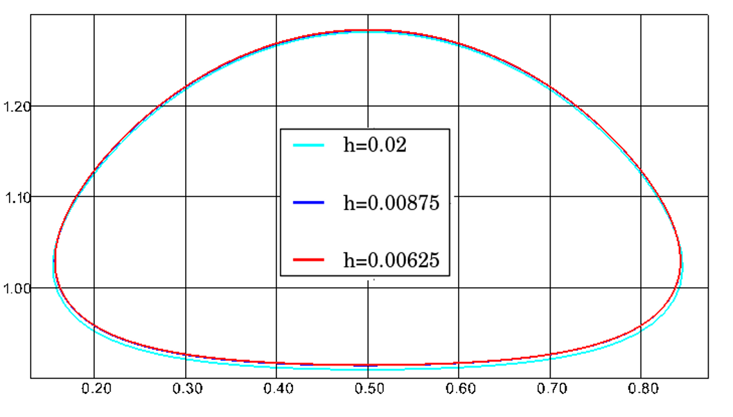
(a) Shape at final time ($t=3$).

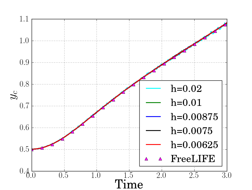
(b) $y_{c}$ vertical position.

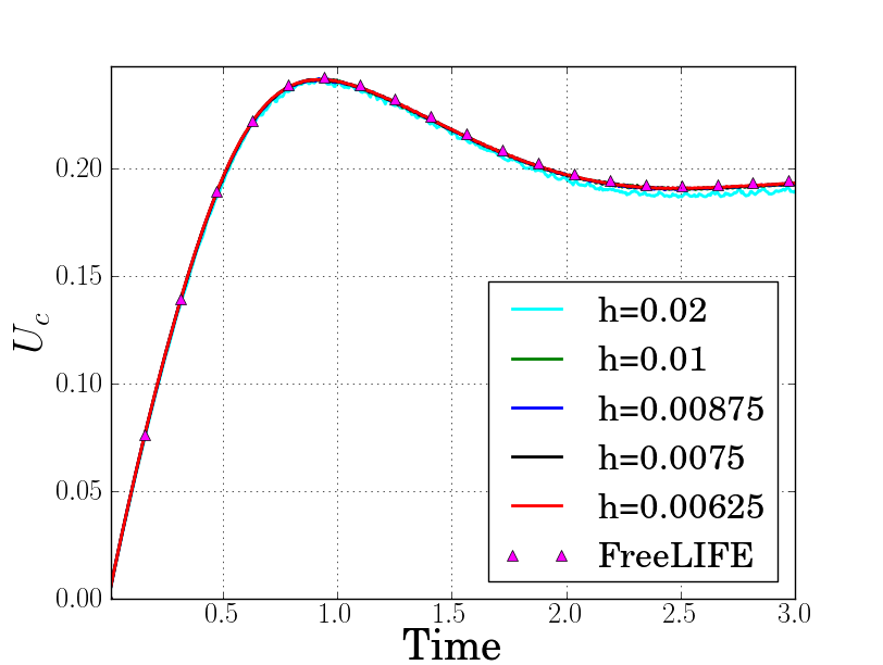
(c) Vertical velocity.

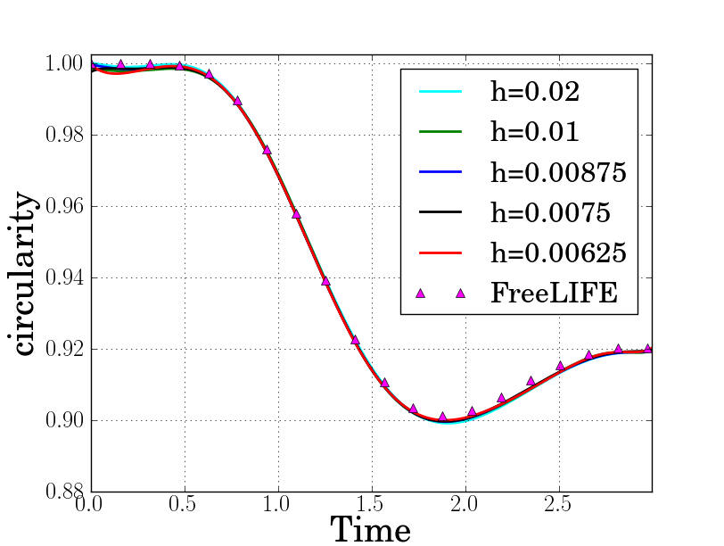
(d) Circularity.

Figure 1: Results for the ellipsoidal bubble

	$c_{min}$	$t_{c_{min}}$	$u_{c_{max}}$	$t_{u_{c_{max}}}$	$y_{c}(t=3)$
lower bound	0.9011	1.8750	0.2417	0.9213	1.0799
upper bound	0.9013	1.9041	0.2421	0.9313	1.0817
h=0.00625	0.9001	1.9	0.2412	0.9248	1.0815
h=0.0075	0.9001	1.9	0.2412	0.9251	1.0812
h=0.00875	0.89998	1.9	0.2410	0.9259	1.0814
h=0.01	0.8999	1.9	0.2410	0.9252	1.0812
h=0.02	0.8981	1.925	0.2400	0.9280	1.0787

Table 2: Results comparison between benchmarks values (lower and upper bounds) and ours for ellipsoidal bubble.

In the second test case, the bubble gets more deformed because of the lower surface tension. Some filaments (skirts) appear at the bottom. The velocity attains two local maximum. Figure 2 displays these results and table 3 shows the comparison with the benchmark results. We monitor the same quantities as in the previous test case except that we add the second maximum velocity $u_{c_{max_{2}}}$, and the time to reach it $t_{u_{c_{max_{2}}}}$.

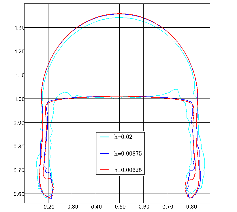
(a) Shape at final time ($t=3$).

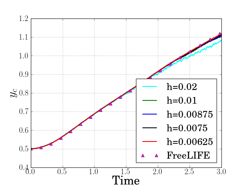
(b) $y_{c}$ vertical.

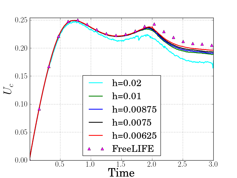
(c) Vertical velocity.

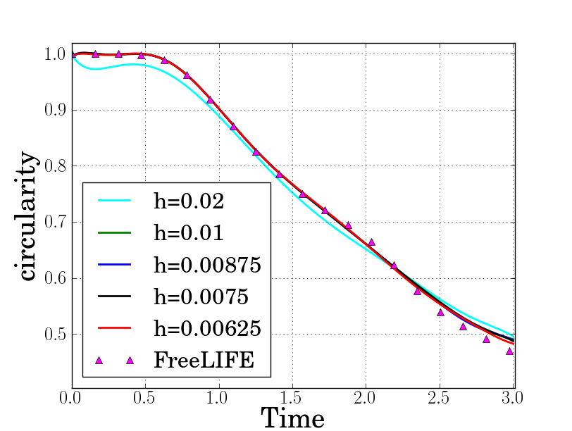
(d) Circularity.

Figure 2: Results for the skirted bubble.

	$c_{min}$	$t_{c_{min}}$	$u_{c_{max_{1}}}$	$t_{u_{c_{max_{1}}}}$	$u_{c_{max_{2}}}$	$t_{u_{c_{max_{2}}}}$	$y_{c}(t=3)$
lower bound	0.4647	2.4004	0.2502	0.7281	0.2393	1.9844	1.1249
upper bound	0.5869	3.0000	0.2524	0.7332	0.2440	2.0705	1.1380
h=0.00625	0.4616	2.995	0.2496	0.7574	0.2341	1.8828	1.1186
h=0.0075	0.4646	2.995	0.2495	0.7574	0.2333	1.8739	1.1111
h=0.00875	0.4629	2.995	0.2494	0.7565	0.2324	1.8622	1.1047
h=0.01	0.4642	2.995	0.2493	0.7559	0.2315	1.8522	1.1012
h=0.02	0.4744	2.995	0.2464	0.7529	0.2207	1.8319	1.0810

Table 3: Results comparison between benchmarks values (lower and upper bounds) and ours for skirted bubble

Both tests show good agreements between our simulations and the ones from the benchmark. We can notice that the final shape of the skirted bubble is very sensitive to the mesh size and none of the groups agree on the exact shape which can explain the differences that we see on the parameters in figure 2 at time $t>2$.

3 Vesicle dynamics simulation

3.1 Model

The model usually admitted for vesicle membrane assumes three properties : (i) the membrane has a bending energy $E_{b}$, called the Canham, Helfrich energy [19, 20], (ii) the inner fluid is incompressible, so the total surface of the vesicle is conserved and finally (iii) the membrane is quasi inextensible, so the local perimeter is conserved over the time.

3.1.1 The bending energy

It has been shown [19, 20] that the bending energy is proportional to the square of the curvature of the membrane, in 2D it reads :

$$E_{b}=\int_{\Gamma}\frac{k_{B}}{2}\kappa^{2},$$ (6)

where $k_{B}$ is the bending modulus (a typical value for phospholipidic membrane is $k_{B}\approx 10^{-19}$ J). Using the virtual power methods, the authors in [3] found a general expression (2D and 3D) for the force associated to this energy. It is given by :

$$\bm{F_{b}}=\int_{\Omega}k_{B}\nabla\cdot\left[\frac{-\kappa^{2}}{2}\frac{\nabla\phi}{|\nabla\phi|}+\frac{1}{|\nabla\phi|}\left(\mathbb{I}-\frac{\nabla\phi\otimes\nabla\phi}{|\nabla\phi|^{2}}\right)\nabla\{|\nabla\phi|\kappa\}\right]\delta_{\varepsilon}.$$ (7)

3.1.2 Membrane inextensibility

The membrane inextensibility is equivalent numerically to impose that the surface divergence of the velocity vanishes on the membrane. Several methods has been developed to impose this constraint using Lagrange multipliers. This idea has been applied with several different methods such as phase field method [21, 3], boundary integral methods [22], and even for level set methods [4, 5]. In particular, in [3], the authors used a phase field method in which the tension is a variable defined in the entire domain and it is given by the solution of an advection equation. This tension is then added to the right hand side of the fluid equations as a force acting on the membrane. The method from [4], is somehow similar to the previous one in the sense that a tension parameter is defined and also added to a membrane force. Then, the system Navier-Stokes with tension equation is solved by a 4 steps projection method discretized by finite differences. In [5], the authors used a level set method solved by FEM in which the Lagrange multiplier is added to the variational formulation of the Navier Stokes equations and acts as a pressure on the membrane to keep the local perimeter constant. Moreover, two Lagrange multipliers are added to the advection equation of the level set in order to maintain constant the surface and the perimeter of the inner fluid. The mesh is finally adaptively refined at each time step around the interface to get improved accuracy.

In the present work, we use a method similar to the one presented in [5]. Indeed, we add a Lagrange multiplier to the fluid equations to impose the constraint (10). But our strategy is to avoid adding Lagrange multipliers on advection equation (which are more difficult to justify physically) and we choose to not adapt the mesh. Instead, we increase the discretization orders to improve the perimeter conservation of the vesicle.

Most of known behaviors of vesicles under flow take place at very low Reynolds number. Thus, we assume that the fluid flow is governed by Stokes equations subject to the inextensibility constraint of the membrane. We have :

$$-2\nu D(\bm{u})+\nabla p = \bm{F}\>\text{ in }\Omega$$ (8)

$$\nabla\cdot\bm{u} = 0\>\text{ in }\Omega$$ (9)

$$\nabla_{s}\cdot\bm{u} = 0\>\text{ on }\Gamma$$ (10)

$$\bm{u} = \bm{g}\>\text{ on }\partial\Omega$$ (11)

with $\bm{u}$ the fluid velocity, $D(\bm{u})=\dfrac{\nabla\bm{u}+\nabla\bm{u}^{T}}{2}$ the deformation tensor, $p$ the pressure, $\bm{F}$ the external forces, and $\nabla_{s}\cdot\bm{u}=\nabla\cdot\bm{u}-(\nabla\bm{u}\cdot\bm{n})\cdot\bm{n}$ the surfacic divergence. The variational formulation associated to the problem (8)-(9)-(10)-(11) reads: Find $(\bm{u},p,\lambda)\in V\times L^{2}_{0}(\Omega)\times H^{1/2}(\Gamma)$ which verify $\forall(\bm{v},q,\mu)\in H^{1}_{0}(\Omega)^{2}\times L^{2}_{0}(\Omega)\times H^{1/2}(\Gamma)$ :

$$2\int_{\Omega}\nu(\phi)D(\bm{u}):D(\bm{v})-\int_{\Omega}p\nabla\cdot\bm{v}+\int_{\Gamma}\lambda\nabla_{s}\cdot\bm{v} = \int_{\Omega}\bm{F}(\phi)\cdot\bm{v},$$ (12)

$$\int_{\Omega}q\nabla\cdot\bm{u} = 0,$$ (13)

$$\int_{\Gamma}\mu\nabla_{s}\cdot\bm{u} = 0,$$ (14)

with $\lambda$ the Lagrange multiplier associated to the free surfacic divergence and $V=\{\bm{v}\in H^{1}(\Omega)^{2}\ |\ \bm{v}|_{\partial\Omega}=\bm{g}\}$. It is obvious in this formulation that the Lagrange multiplier can be interpreted as a pressure acting on the interface.

The problem (12)-(13)-(14) is coupled with the level set advection (2) and discretized using the finite element method. Thereby we introduce ${\mathbb{U}}_{h}^{n+1}$, ${\mathbb{P}}_{h}^{n}$, ${\mathbb{Q}}_{h}^{m}$ ans ${\mathbb{R}}_{h}^{k}$ the discrete finite elements spaces depending on mesh size $h$ and based on Lagrange polynomials of degree $n+1$, $n$, $m$ and $k$ for the velocity, pressure, Lagrange multipliers and levelset respectively. A complete description of the strategy to obtain high order level set method (including reinitialization at high order and benchmarks) will be presented in [23]. Let $(\bm{u}_{h},p_{h},\lambda_{h},\phi_{h})\in{\mathbb{U}}_{h}^{n+1}\times{\mathbb{P}}_{h}^{n}\times{\mathbb{Q}}_{h}^{m}\times{\mathbb{R}}_{h}^{k}$ be the discretization of $(\bm{u},p,\lambda,\phi)$. The discrete version of (12)-(13)-(14)-(2) reads: Find $(\bm{u}_{h},p_{h},\lambda_{h},\phi_{h})\in{\mathbb{U}}_{h}^{n+1}\times{\mathbb{P}}_{h}^{n}\times{\mathbb{Q}}_{h}^{m}\times{\mathbb{R}}_{h}^{k}$ which verify $\forall(\bm{v}_{h},q_{h},\mu_{h},\psi_{h})\in{\mathbb{U}}_{h}^{n+1}\times{\mathbb{P}}_{h}^{n}\times{\mathbb{Q}}_{h}^{m}\times{\mathbb{R}}_{h}^{k}$ :

$$2\int_{\Omega}\nu(\phi_{h})D(\bm{u}_{h}):D(\bm{v}_{h})-\int_{\Omega}p_{h}\nabla\cdot\bm{v}_{h}+\int_{\Omega}\lambda_{h}\nabla_{s}\cdot\bm{v}_{h}\ \delta_{\varepsilon}(\frac{\phi_{h}}{|\nabla\phi_{h}|}) = \int_{\Omega}\bm{F}_{h}\cdot\bm{v}_{h},$$ (15)

$$\int_{\Omega}q_{h}\nabla\cdot\bm{u}_{h} = 0,$$ (16)

$$\int_{\Omega}\mu_{h}\nabla_{s}\cdot\bm{u}_{h}\ \delta_{\varepsilon}(\frac{\phi_{h}}{|\nabla\phi_{h}|}) = 0,$$ (17)

$$\int_{\Omega}\frac{\partial\phi_{h}}{\partial t}\psi_{h}+\int_{\Omega}(\bm{u}_{h}\cdot\nabla\phi_{h})\psi_{h}+\int_{\Omega}S(\phi_{h},\psi_{h}) = 0.$$ (18)

Note that we replaced the integral over $\Gamma$ by integral over $\Omega$ thanks to the delta function. Thus, the Lagrange multiplier space is defined only in the elements in a region of $2\varepsilon$ around the interface $\phi=0$. In practice, from the implementation point of view, we only add to the global matrix the coefficients that correspond to these “few” elements.

3.2 Tank treading motion

The first behavior on which we validate our model is the tank treading motion (TT). In a linear shear flow, if the viscosity ratio between the inner and outer fluids $\nu_{r}=\dfrac{\nu_{2}}{\nu_{1}}$ is lower than a critical value, the vesicle reaches a steady angle with respect to the horizontal. At the same time, the membrane is rotating along the vesicle with a constant velocity (this motion is similar to the chain of a tank hence the name tank treading motion).

We need to define dimensionless parameters which control this system: (i) the reduced area $\alpha$ is the ratio between the area of the vesicle ($A$) and the area of a circle having the same perimeter ($P$) $\bigg{(}\alpha=\dfrac{4\pi A}{P^{2}}\bigg{)}$, (ii) the capillary number $C_{a}$ which is the ratio between the characteristic time of the shear $(\frac{1}{\gamma})$ and a characteristic time related to the curvature force, it is given by $C_{a}=\dfrac{\nu_{2}\gamma R_{0}^{3}}{k_{B}}$ with $R_{0}=\dfrac{P}{2\pi}$ stands for a typical size of the vesicle. For high values of $C_{a}$, the particle is more deformable due to the hydrodynamic forces, while for low $C_{a}$, the Helfrich energy requires a higher cost to change the curvature of the vesicle. The confinement $c$ is defined as the ratio between the equivalent radius of the vesicle and the half width of the channel : $c=\dfrac{R_{0}}{L/2}$.

Figure 3 shows the initial and steady states of a vesicle in a shear flow with $\alpha=0.8$, $C_{a}=0.12$ and $c=0.6$. Initially, the vesicle is placed horizontally and initialized as an ellipse. At steady state, the vesicle has taken a steady angle with respect to the horizontal, and the fluid velocity rotates along the membrane (this is shown by streamlines in figure 3(b)). The simulation has been run in a rectangular box of size $[10,2.12]^{2}$ descretized by $12400$ elements. The time step was taken as $\delta t=5\times 10^{-3}$ and the finite elements discretization space was ${\mathbb{U}}_{h}^{3}\times{\mathbb{P}}_{h}^{2}\times{\mathbb{Q}}_{h}^{2}\times{\mathbb{R}}_{h}^{2}$.

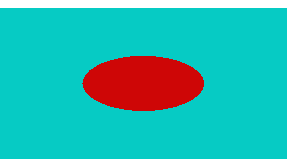
(a) $t=0$

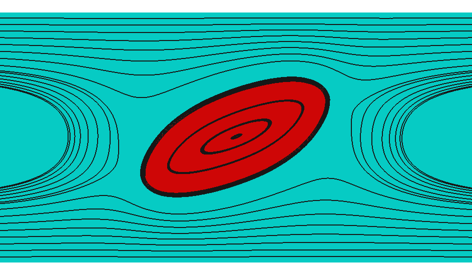
(b) $t=5$

Figure 3: Vesicle at $\alpha=0.8,C_{a}=0.12\text{ and }c=0.6$ reaches a steady angle. Streamlines are along the membrane, the vesicle is under tank treading regime.

Different finite element discretization has been tested. Figure 4 shows the results of three different sets of polynomials orders $(n,m,k)$ : $(1,1,1)$, $(2,2,2)$ and $(3,3,3)$. The computational time is multiplied by $2$ from $(n,m,k)=(1,1,1)$ to $(n,m,k)=(2,2,2)$ and multiplied by $4$ from $(n,m,k)=(1,1,1)$ to $(n,m,k)=(3,3,3)$. We can see on figure 4(a) that the tank treading steady angle doesn’t change dramatically for simulations up to this final time. Nevertheless, the loss of perimeter is a crucial point for accuracy in long time simulations. Thus, we plotted in figure 4(b) the loss of perimeter : $\dfrac{|p-p_{0}|}{p_{0}}\times 100$ for the different polynomial approximations used. The oscillations seen on figure 4(b) are due to the reinitialization steps. One can see that increasing the polynomial order approximation improves the conservation of the perimeter. The exact role of each polynomial approximation on the perimeter conservation accuracy still has to be investigated. For the other simulations, we choose to take $(n,m,k)=(2,2,2)$ as polynomial order approximation which, for our applications, seems to be a good compromise between accuracy and computational time.

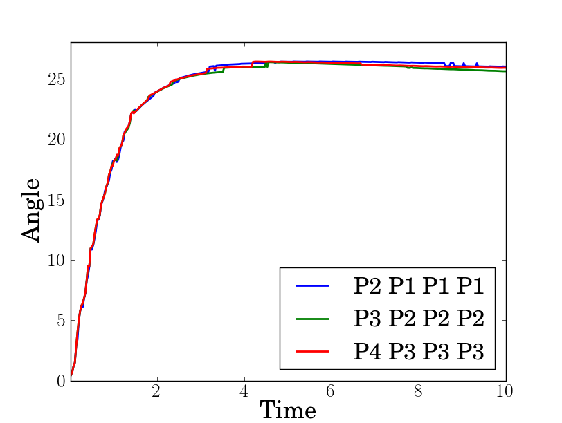
(a) Vesicle angle

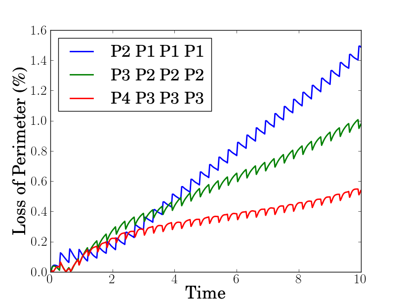
(b) Loss of perimeter (in %)

Figure 4: Vesicle angle and loss of perimeter for different polynomial approximation order. The legend gives in this order : $(n+1,n,m,k)$.

It has been shown in [1] that the steady tank treading angle decreases with the reduced area. So, we run the same simulation than shown in 3 by changing the reduced area of the vesicle. The steady angles exhibit the expected behavior as one can see it in figure 5(a).

Moreover, it has been also shown in [1] that for a given reduced area, the steady angle is lower for high confinements. Figure 5(b) shows the steady angles that we found for three different confinements at different reduced volumes. Once again, we obtain the expected behavior.

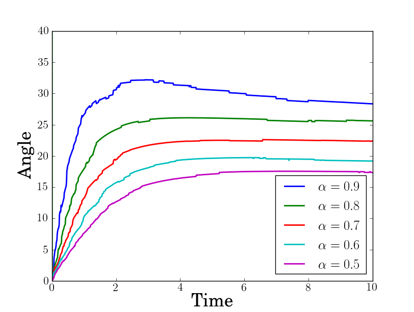
(a) Vesicle angle in shear flow for $c=0.6$ and $C_{a}=0.1$

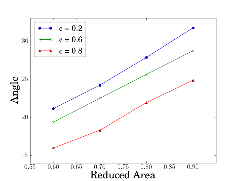
(b) Steady angle of vesicle in tank treading motion as a function of reduced area for different confinements.

Figure 5: Vesicle angle as a function of time, reduced area and confinement.

3.3 Tumbling motion

When the viscosity ratio $\nu_{r}$ is above a critical value, the vesicle tends to follow a solid rotation, it is called the tumbling motion. Increasing the viscosity ratio increases the rotation frequency of the vesicle.

To reproduce this behavior, we set initially a vesicle as an ellipse in a box of size $[14,5]^{2}$, discretized with $7218$ elements. We chose a time step of $\delta t=3\times 10^{-2}$. These parameters are not as refined than in the previous section in order to get long time simulations in a reasonable computational time. The other parameters of the simulation were : $C_{a}=6\times 10^{-2}$, $c=0.25$ and $\alpha=0.8$. Figure 6 displays the tumbling motion.

Increasing the viscosity ratio increases the rotation frequency of the tumbling as it can be seen on figures 7(a) and 7(b). Moreover, as described in [24], when one increases the viscosity ratio, the rotation frequency of the vesicle reaches a steady value which corresponds to the steady rotation of a solid object in a shear flow. We can see this phenomenon in figure 7(b).

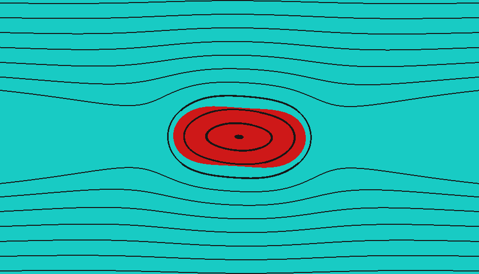
(a) $t=1.0$

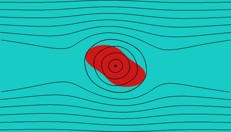
(b) $t=1.1$

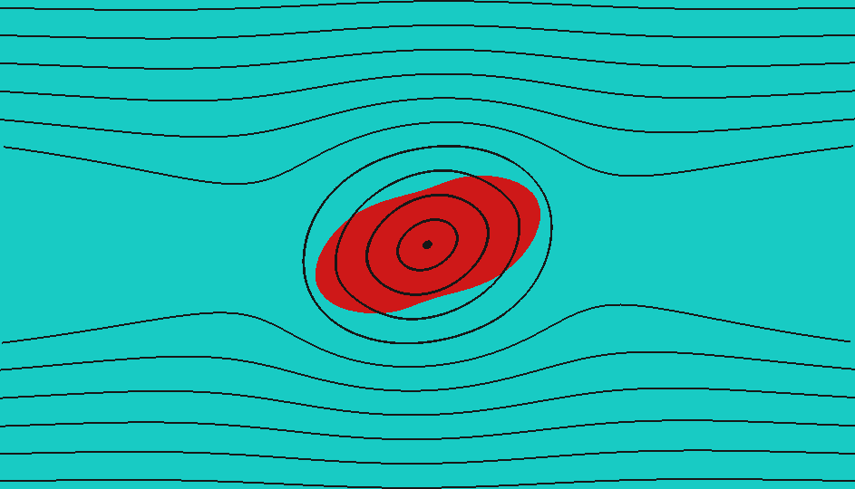
(c) $t=6.0$

Figure 6: Tumbling of a vesicle

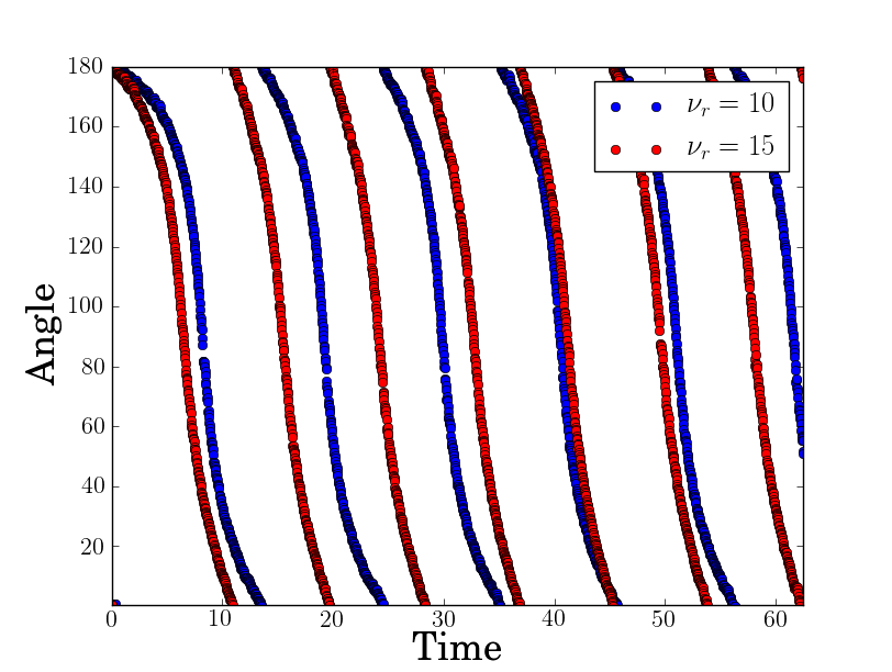
(a) Tumbling angle as a function of time for two different viscosity ratios.

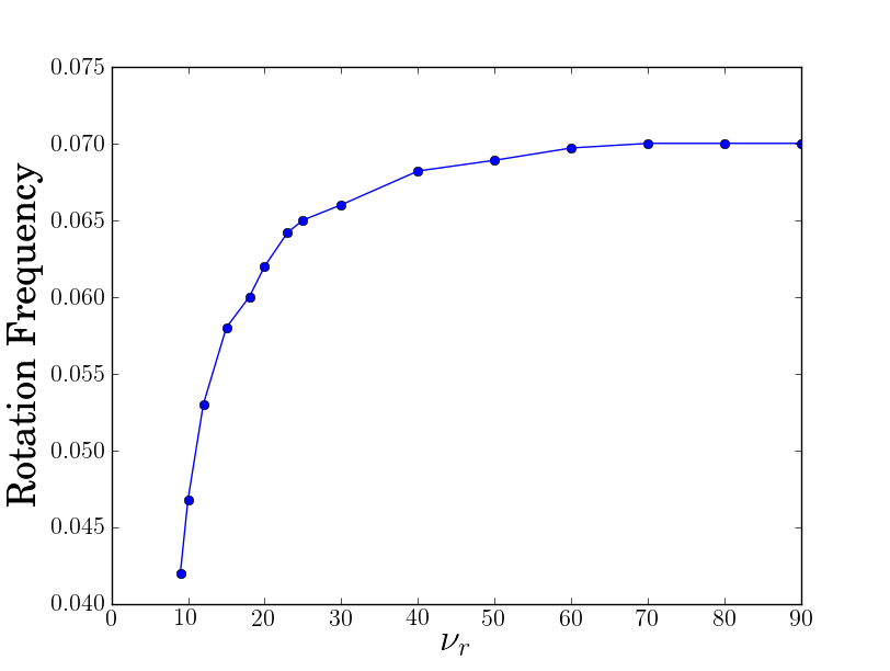
(b) Tumbling frequency for different viscosity ratios.

Figure 7: Tumbling angle and frequency.

Conclusion

We have presented a new numerical framework for the simulation of vesicle under flow. This framework is based on level set methods solved by a (possibly high order) finite element method. First the level set framework for two-fluid flows at order $(1,1,1)$ has been verified using a numerical benchmark. Then, for more complex entities such us vesicles, the incompressibility of the membrane is taken into account using a Lagrange multiplier defined on the interface. Compared to the literature, one of the novelties of our work lies in the possibility of taking into account this constraint without refining the mesh or introducing auxiliary variables. This being done at a lower cost in the sense that this multiplier affects only the elements crossed by the interface.

A validation on tank treading and tumbling regimes has been presented. In particular, for the tank treading motion we have used high order polynomial approximations $(2,2,2)$ and $(3,3,3)$. However, a theoretical study of the role of each approximation order and its verification on numerical tests has to be done in a near future. Finally other basic behaviors of vesicles under flow has been tested for a polynomial order of $(2,2,2)$ and show the expected results in good agreement with the literature.

We are also interested in clustering phenomenon which is very important in the case of red blood cells and also to do 3D calculations (the FEEL++ library allows it without much changes in the code).

References

References

- [1] B. Kaoui, J. Harting, C. Misbah, Two-dimensional vesicle dynamics under shear flow: Effect of confinement, pre 83 (6) (2011) 066319–+. arXiv:1011.6061, doi:10.1103/PhysRevE.83.066319.
- [2] J. Beaucourt, F. Rioual, T. Seacuteon, T. Biben, C. Misbah, Steady to unsteady dynamics of a vesicle in a flow, Phys. Rev. E 69 (1) (2004) 011906–.
- [3] E. Maitre, C. Misbah, P. Peyla, A. Raoult, Comparison between advected-field and level-set methods in the study of vesicle dynamics, ArXiv e-printsarXiv:1005.4120.
- [4] D. Salac, M. Miksis, A level set projection model of lipid vesicles in general flows, Journal of Computational Physics 230 (22) (2011) 8192–8215.
-
[5]
A. Laadhari, P. Saramito, C. Misbah,
Computing the
dynamics of biomembranes by combining conservative level set and adaptive
finite element methods, cNRS (Jun. 2011).
URL http://hal.archives-ouvertes.fr/hal-00604145/en/ - [6] M. Ismail, A. Lefebvre, A “necklace” model for vesicles simulation in 2d, submitted to Journal of Computational Physics (2012).
- [7] C. Winkelmann, Interior penalty finite element approximation of navier-stokes equations and application to free surface flows, Ph.D. thesis (2007).
- [8] S. Osher, J. A. Sethian, Fronts propagating with curvature dependent speed: Algorithms based on hamilton-jacobi formulations, Journal of computational physics 79 (1) (1988) 12–49.
- [9] J. Sethian, Level Set Methods and Fast Marching Methods, Cambridge University Press, 1996.
- [10] R. F. Stanley Osher, Level Set Methods and Dynamic Implicit Surfaces, Springer, S.S. Antman, J.E. Marsden, L. Sirovich.
- [11] E. M. Georges-Henri Cottet, A level set method for fluid-structure interactions with immersed surfaces, Mathematical Models and Methods in Applied Sciences.
-
[12]
C. Prud’Homme, V. Chabannes, V. Doyeux, M. Ismail, A. Samake, G. Pena,
Feel++: A Computational
Framework for Galerkin Methods and Advanced Numerical Methods, submitted to
ESAIM Proc. (Jan. 2012).
URL http://hal.archives-ouvertes.fr/hal-00662868 - [13] C. Prud’homme, V. Chabannes, G. Pena, Feel++: Finite Element Embedded Language in C++, Free Software available at http://www.feelpp.org, contributions from A. Samake, V. Doyeux, M. Ismail and S. Veys.
- [14] C. Prud’homme, A domain specific embedded language in C++ for automatic differentiation, projection, integration and variational formulations, Scientific Programming 14.
- [15] L. P. Franca, S. L. Frey, T. J. Hughes, Stabilized finite element methods: I. application to the advective-diffusive model, Computer Methods in Applied Mechanics and Engineering 95 (2) (1992) 253–276.
- [16] E. Burman, P. Hansbo, Edge stabilization for the generalized stokes problem: A continuous interior penalty method, Computer Methods in Applied Mechanics and Engineering 195 (19-22) (2006) 2393–2410.
- [17] V. Chabannes, G. Pena, C.Prud’homme, High order fluid structure interaction in 2d and 3d. application to blood flow in arteries, in: Fifth International Conference on Advanced COmputational Methods in ENgineering (ACOMEN 2011), 2011.
- [18] S. Hysing, S. Turek, D. Kuzmin, N. Parolini, E. Burman, S. Ganesan, L. Tobiska, Quantitative benchmark computations of two-dimensional bubble dynamics, International Journal for Numerical Methods in Fluids 60 (11) (2009) 1259–1288. doi:10.1002/fld.1934.
- [19] P. Canham, The minimum energy of bending as a possible explanation of the biconcave shape of the human red blood cell, Journal of Theoretical Biology 26 (1) (1970) 61 – 81. doi:DOI:10.1016/S0022-5193(70)80032-7.
- [20] W. Helfrich, Elastic properties of lipid bilayers: theory and possible experiments., Z Naturforsch C 28 (11) (1973) 693–703–.
- [21] D. Jamet, C. Misbah, Towards a thermodynamically consistent picture of the phase-field model of vesicles: Local membrane incompressibility, Phys. Rev. E 76 (5) (2007) 051907. doi:10.1103/PhysRevE.76.051907.
- [22] S. K. Veerapaneni, D. Gueyffier, D. Zorin, G. Biros, A boundary integral method for simulating the dynamics of inextensible vesicles suspended in a viscous fluid in 2d, Journal of Computational Physics 228 (7) (2009) 2334 – 2353. doi:10.1016/j.jcp.2008.11.036.
- [23] V. Doyeux, C. Prud’homme, M. Ismail, A framework toward high order level set method., in preparation.
- [24] G. Ghigliotti, T. Biben, C. Misbah, Rheology of a dilute two-dimensional suspension of vesicles, Journal of Fluid Mechanics 653 (2010) 489–518. doi:10.1017/S0022112010000431.