Tunable filter imaging of high redshift quasar fields

Abstract

We have used the Taurus Tunable Filter to search for Lyman $\alpha$ emitters in the fields of three high redshift quasar fields: two at $z\sim 2.2$ (MRC B1256-243 and MRC B2158-206) and one at $z\sim 4.5$ (BR B0019-1522). Our observations had a field of view of around 35 square arcminutes, and reached AB magnitudes of magnitudes of $\sim$21 (MRC B1256-243), $\sim$22 (MRC B2158-206), and $\sim$22.6 (BR B0019-1522), dependent on wavelength. We have identified candidate emission line galaxies in all three of the fields, with the higher redshift field being by far the richest. By combining our observations with simulations of the instrumental response, we estimate the total density of emission line galaxies in each field. Seventeen candidate emission line galaxies were found in within 1.5 Mpc of BR0019-1522, a number density of $4.9\pm 1.2\times 10^{-3}$ Mpc^-3, suggesting a significant galaxy overdensity at $z\sim 4.5$.

1 Introduction

Table 1: Details of the observations made of each target. Standard stars (HD49798, EG 274 and EG 21) for photometric calibration were observed with the same instrumental configuration.

Target	Redshift	Position (J2000)		Date	Exposure	Axial	Comment
		RA	Dec		Time (s)	Wavelength (Å)
MRC B1256-243	2.263	12h59m12.6s	-24°36’05”	2003 July 27	15 $\times$ 60	3957.2	Repeated
						3967.1	twice.
						3977.1
						3987.1
MRC B2158-206	2.249	22h01m27.0s	-20°25’36”	2003 July 27	15 $\times$ 60	3959.1	Repeated
						3969.1	four
						3979.1	times.
						3989.0
						3999.0
BR B0019-1522	4.528	00h22m08.0s	-15°05’39”	1997 Nov. 6	600	6709.5	Repeated
						6725.9	eight
						6742.3	times.

The evolution of clustering with cosmic time is widely recognised as one of the most rigid tests of the cold dark matter paradigm (Kaiser, 1991; Springel et al., 2005). However, locating high redshift clusters is challenging. The traditional methods of X-ray and blind optical searches are limited: X-ray surveys can detect only the most luminous sources at high-$z$, while optical searches are highly vulnerable to projection effects. In order to overcome these limitations, a way of targeting the search is needed.

Since the earliest studies, it has been established that quasars are associated with groups and clusters of galaxies (Bahcall et al., 1969; Oemler et al., 1972). More recently, McLure & Dunlop (2001) argued that a close match between the space density of clusters and that of quasars indicates that practically all clusters contained an AGN at high redshift. Further, Rawlings & Jarvis (2004) propose that radio jets from AGN are a major influence on cluster evolution. They suggest that a galaxy merger within the cluster triggers a radio-jet episode; the jets then delivery energy to the intracluster medium, heating it and preventing it from falling into the other developing cluster galaxies. These galaxies are thus starved of fuel, and star formation within the cluster will effectively shut down. Rawlings & Jarvis speculate that every protocluster undergoes such an episode, strengthening the link postulated by McLure & Dunlop.

This relationship between galaxy overdensities and AGN suggests a method for locating high-$z$ clusters: we can use quasars as convenient ‘anchors’ for our search. This technique has already been exploited by others with notable success: for example, Stiavelli et al. (2005) tentatively report the detection of clustering around a radio-quiet quasar at $z=6.28$.

To date most galaxy clusters detected around AGN have been identified based on statistical overdensities of objects observed in their vicinity. A better strategy for overcoming foreground contamination is to identify individual star forming galaxies in the AGN field by their characteristic redshift dependent features. In particular, Lyman $\alpha$ emission has been used to identify high redshift galaxies for some time. Among the first high redshift objects identified by emission lines were the $z=4.55$ Ly $\alpha$ emitters observed in the field of the quasar BR B2237-0607 by Hu & McMahon (1996). Since then, a series of highly profitable observations of Ly $\alpha$ emitters in AGN fields have been carried out. Kurk et al. (2000) and Pentericci et al. (2000) used a combination of narrow- and broad-band imaging with follow-up spectroscopy to identify a galaxy overdensity within 1.5 Mpc of the $z=2.156$ radio galaxy PKS B1138-262. Similar results have been achieved for the radio galaxies TN J1338-1942 ($z=4.1$; Venemans et al., 2002), TN J0924-2201 ($z=5.2$; Venemans et al., 2004; Overzier et al., 2006) and MRC B0316-257 ($z=3.13$; Venemans et al., 2005) and 6C0140+326 ($z=4.413$; Kuiper et al., 2011).

While this combination of broad and narrowband imaging has produced demonstrably successful results, the more direct antecedents of this work have adopted an alternative approach. The Taurus Tunable Filter (TTF) instrument, installed on the Anglo-Australian Telescope, provided a powerful method of narrow-band (of order 10 Å) imaging over a large range of wavelengths (Bland-Hawthorn & Jones, 1998). Bremer & Baker (1999) introduced the strategy used to search for line emitters at a given redshift with TTF: broadly, the tunable filter is stepped across a range of wavelengths around the expected redshifted position of the emission. Emission line galaxies then appear brighter in those frames centred on the spectral line.

Considerable success has been achieved at lower redshifts with this technique. Baker et al. (2001) located a cluster around the $z=0.9$ radio-loud quasar MRC B0450-221 using TTF to search for $[$O ii$]$ 3727 Å emission. The same technique was used by Barr et al. (2004), who examined six radio-loud quasars at redshifts $0.8<z<1.3$, identifying a total of 47 candidate emission line galaxies (ELGs), at an average space density around 100 times higher than that found locally.

Further work with TTF was performed by Francis & Bland-Hawthorn (2004), who targeted Ly $\alpha$ emitters within 1 Mpc of the $z=2.159$ radio loud quasar PKS B0424-131 without making any detections. These authors selected this extremely luminous UV source with the expectation of finding Ly $\alpha$ fluorescent clouds in the vicinity of the quasar but these were not detected. With specific application to PKS B0424-131, Bruns et al. (2011) demonstrated that the most intrinsically UV-luminous quasars observed beyond $z=1$ suppress star formation in low-mass haloes ($M_{\rm vir}\lesssim 10^{12}$ M_⊙) within a megaparsec of the quasar. The intense UV radiation field is expected to photo-evaporate HI clouds which presumably accounts for the lack of detections. We return to this point in our conclusion (§ 6).

The present work continues to push TTF to higher redshifts, searching three quasar fields at redshifts up to $z\sim 4.5$. The objects selected include examples of both radio-loud and radio-quiet quasars, and their environments are compared. Section 2 of this paper describes the observations, including target selection, instrumental characteristics and a note on data reduction. Section 3 describes simulations performed to examine statistical properties and completeness of our sample. Section 4 describes how candidate ELGs were identified and presents details on the detections, as well as considering the possible sources of mis-identified ‘interloper’ objects. Section 5 analyses the distribution and properties of the sample. Our conclusions are summarised in Section 6. Throughout, we assume an $H_{0}=70$ km s^-1 Mpc^-3, $\Omega_{\Lambda}=0.7$, $\Omega_{\mathrm{M}}=0.3$ cosmology.

2 Observations

2.1 Target selection

Two data sources were used for this analysis. The authors used TTF to observe objects drawn from the Molonglo Quasar Sample (MQS; Kapahi et al., 1998) of low-frequency-selected radio-loud quasars in July 2003. Six targets had been selected from the MQS on the basis of observability, suitable redshifts being limited by the necessity to place Lyman $\alpha$ within the wavelength ranges accessible to TTF’s order-blocking filters. Due to weather constraints, only two quasars were observed: MRC B1256-243 ($z=2.263$) and MRC B2158-206 ($z=2.249$). Immediately following each quasar observation, a standard star was observed with the same instrumental settings for flux calibration. In addition, observations of BR B0019-1522, a $z=4.528$ radio-quiet quasar, were drawn from the Anglo-Australian Observatory archive. These data were taken on 1997 November 6 by Bland-Hawthorn, Boyle and Glazebrook, and were accompanied by companion observations of a standard star. Details of each target are given in Table 1.

2.2 Instrumental setup and characteristics

Throughout this work, a distinction is drawn between a frame (corresponding to one set of data read from the CCD), an image (a number of frames at the same etalon settings which have been combined for analysis) and a field, or stack of images of the same area of sky at different etalon settings.

2.2.1 Wavelength variation and the optical axis

Fabry-Pérot images have a quadratic radial wavelength dependence of the form $\lambda_{\theta}=\lambda_{centre}(1-\theta^{2}/2)$ (Bland & Tully, 1989), where $\theta$ is the off-axis angle at the etalon. In a typical observation, the wavelength varies across the field by around 1% of $\lambda_{centre}$. Wavelength calibration is performed with respect to the axial wavelength; for any given pixel position on the image, it is then possible to calculate the wavelength observed at that point.

2.2.2 Objects at $z\sim 2.2$

The TTF was used at $f/8$ on the AAT in combination with the EEV2 CCD. This resulted in a scale of 0.33” per pixel. After processing, the total useful rectangular field of view in the observations was around 7’ by 5’. The radial wavelength variation described in Section 2.2.1 resulted in a shift of 1.4 Å at 2’ from the optical axis and 6.7 Å at 4’ from the axis. Conditions were photometric, and seeing was on the order of 1.5”. The full width at half maximum of the etalon transmission band was 7.5 Å.

The targets were scanned at etalon plate spacings corresponding to a series of wavelength steps of approximately 10 Å, the aim being to straddle the redshifted Ly $\alpha$. However, an intermediate-band order-blocking filter is necessary to eliminate unwanted wavelengths and other orders of interference. In this case, the AAT’s B1 filter was the best available. Unfortunately, the observed wavelengths were at the very edge of the filter transmission, as shown in Fig. 1: the signal to noise ratio therefore decreases significantly with wavelength. Table 1 and Fig. 1 record observations of MRC B1256-243 at 3987.1 Å. When these data were analysed, it was clear that the reduced filter transmission had resulted in no useful results at this wavelength. These data are not considered further in this work. The MRC B2158-206 observations at 3989.0 Å and 3999.0 Å are included hereafter, but did not include any useful detections.

Each CCD frame contained a total of 30 minutes of observations, taken at two separate axial wavelengths. Each wavelength was exposed for 60 seconds a total of 15 times. This procedure was repeated twice in the case of MRC B1256-243 and four times for MRC B2158-206; the total exposure times at each wavelength are thus 30 minutes and 1 hour, respectively. Between each image, the telescope pointing was shifted slightly: this enabled the easy identification and subsequent elimination of diametric ghosts in the data.

2.2.3 Objects at $z\sim 4.5$

The TTF was used at $f/8$ on the AAT in combination with the MITLL2 CCD. This resulted in a scale of 0.37” per pixel. After processing, the total useful rectangular field of view in the observations was 9’17” by 4’10”. The radial wavelength variation described in Section 2.2.1 resulted in a shift of 5.1 Å at 2’ from the optical axis and 20.3 Å at 4’ from the axis. Conditions were photometric, and the seeing was on the order of 1.5”. The full width at half maximum of the etalon transmission band was 9.5 Å. The AAT’s R0 intermediate-band order-blocking filter was used: this provided effectively constant transmission across the wavelength range under consideration.

Each CCD frame contained a total of 30 minutes of observations: ten at each of three axial wavelengths. Eight CCD frames were recorded, resulting in a total of 80 minutes exposure for each axial wavelength. As before, the telescope position was shifted slightly between images.

Figure 1: On-axis etalon transmission bands for each of the three fields observed shown relative to the relevant order-blocking filter used on the telescope. Away from the optical axis the etalon transmission shifts to shorter wavelengths (§2.2.1).

2.3 Data reduction and catalogue construction

Data reduction proceeds broadly as for standard broadband imaging. A full consideration of the issues surrounding tunable filter data is given by Jones & Bland-Hawthorn (2001) and Jones et al. (2002). The various different images of each field at the same axial wavelengths were aligned by a marginal centroid fit on bright stars and then combined. Wavelength calibration was performed through an emission line, as described by Jones et al.; xenon and copper-helium arc lamps were used for the $z\sim 2.2$ fields, and a neon arc lamp for BR B0019-1522.

After the data had been reduced, object detection and fixed aperture photometry were performed on each image using SExtractor (Bertin & Arnouts, 1996). The object detection parameters were defined as described in the next section.

2.4 Photometry

The observations of the standard stars were reduced in the same way. For each star, SExtractor was used to perform aperture photometry yielding a count $C_{\mathrm{s}}$. This corresponds to a known magnitude $m_{\mathrm{s}}$, based on Hamuy et al. (1992) for the lower redshift fields or from the ESO Standard Star Catalogue for that of BR B0019-1522. If the exposure time on the standard is $t_{\mathrm{s}}$ and that on an object in the field is $t_{\mathrm{Obj}}$, the AB magnitude of the object is

$$m_{\mathrm{AB}}=m_{\mathrm{s}}-2.5\log_{10}(C_{\mathrm{Obj}}t_{\mathrm{s}})/(C_{\mathrm{s}}t_{\mathrm{Obj}}).$$ (1)

The AB magnitude system (Oke, 1974) is defined by $m_{\mathrm{AB}}=-2.5\log_{10}f_{\nu}-48.60$ where $f_{\nu}$ is the flux in units of ergs cm^-2 s^-1 Hz^-1. The monochromatic flux $f_{\lambda}$, in units of ergs cm^-2 s^-1 Å^-1, is then

$$f_{\lambda}=(c\times 10^{-\left(m_{\mathrm{AB}}+48.60\right)/2.5})/\lambda^{2}.$$ (2)

Conversion from $f_{\lambda}$ to the total flux in the band, $f_{\mathrm{total}}$ is performed by multiplying by the effective width of the etalon transmission. The etalon transmission band may be taken as Lorentzian, normalised to 1 at the wavelength of peak transmission, thus:

$$T(\lambda)=(\lambda_{\nicefrac{{1}}{{2}}}^{2}/4)/((\lambda-\lambda_{\mathrm{c}})^{2}+\lambda_{\nicefrac{{1}}{{2}}}^{2}/4)$$ (3)

where $\lambda$ is the wavelength, $\lambda_{c}$ the central wavelength of the band and $\lambda_{\nicefrac{{1}}{{2}}}$ its full width at half maximum. Assuming that $\lambda_{\mathrm{c}}\gg\lambda_{\nicefrac{{1}}{{2}}}$, Equation 3 may be integrated over $0\leq\lambda\leq\infty$ to yield a width of $\pi\lambda_{\nicefrac{{1}}{{2}}}/2$. Combining this with Equation 2 yields a total flux in the band of

$$f_{\mathrm{total}}=(\pi c\lambda_{\nicefrac{{1}}{{2}}}\times 10^{-\left(m_{\mathrm{AB}}+48.60\right)/2.5})/2\lambda_{\mathrm{c}}^{2}$$ (4)

with units ergs cm^-2 s^-1.

It is worth noting that this measures the flux received in the etalon passband, and is thus a lower limit of the line flux of the ELG: variations of line shapes and widths, and their positions relative to the etalon passband, will cause the fluxes measured to be systematically underestimated. They should therefore be regarded as lower limits.

3 Simulations

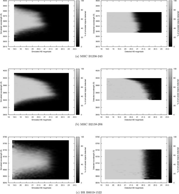
Figure 2: Depths of each of the three fields as determined by the simulations described in Section 3.2.2. On the left, the data is plotted in terms of simulation inputs; on the right, in terms of the measurements made from the simulated images. Note that the effects of the blocking filter are clearly seen in the two upper (lower redshift) fields, as the completeness tails off at higher wavelength. The higher redshift BR B0019-1522 field falls well within the blocking filter, so the depth is relatively constant with wavelength across the observed range.

We constructed a series of simulated images: data with properties similar to our observations, but containing a known population of objects. The analysis of these enables us to address the following questions:

• What are the most appropriate SExtractor parameters for extracting useful data from the images?

• To what depth is each field complete–and how does that vary over the field?

• To what extent is our analysis prone to mis-identifying spurious ‘noisy’ features in an image as candidate emission line galaxies?

3.1 Construction of simulated images

Images were simulated in two stages: first, a background was generated, then objects were superimposed on top of it.

Due to the properties of the blocking filter and the variation of wavelength across the image, the background signal is not constant across the image. Each data image was therefore divided into 100 by 100 pixel blocks, and the mean background signal and associated noise was measured in each block. Simulated blocks were then generated matching each of these, and then recombined to form an overall simulated background of the same shape as the data.

A Ruby code was written to simulate the expected properties of objects we might observe. Objects were simulated at random redshifts (over the range the observations might be expected to cover) and pixel positions within the images. Based on the work of Le Delliou et al. (2006), our observations were not expected to be sensitive to continuum emission from ELGs, so this was not considered. Further, the ELGs are spatially unresolved, so were simulated with a Gaussian point spread function equal to the measured seeing. An emission line model was developed based on the widths and profiles of high-$z$ Lyman $\alpha$ emitters based chiefly on the $z\sim 4.5$ objects observed by Dawson et al. (2004). Experimentation suggested that the results obtained were not sensitive to line profile; velocity widths in the range 100–1000 km s^-1 were chosen based on both Dawson et al. (2004) and the more extreme example documented by Tapken et al. (2004).

The effects of the instrument on the objects’ detectabilty were then considered before they were added to the background images. First a correction for the order-blocking filter transmission was applied, using the position of the object within the field to determine the observed wavelength and hence filter transmission. The line profile was then multiplied by the transmission profile of the etalon for the image under construction.

3.2 Results of simulations

Following the procedure above, simulations were run of all three fields. For each data image, a total of 500 simulated images were constructed, each containing 500 simulated sources.

3.2.1 Detection parameters

Source extraction was run multiple times on each image with different SExtractor configuration parameters. In each case, the results were compared with the catalogue of simulated objects in the image. The combination of parameters that produced the greatest number of detections of known objects combined with the smallest number of spurious detections of noise were then used for the analysis of both the simulations and the observed data. These parameters are listed in Table 2.

Table 2: Optimal SExtractor parameters determined by simulations and used throughout this work.

Parameter	Value	Description
detect_minarea	06.0	Minimum number of pixels per detection.
detect_thresh	01.3	Detection threshold in $\sigma$ above local background.
back_size	64.0	Size in pixels of mesh used for background estimation.
phot_apertures	06.0	Aperture diameter (pixels).

3.2.2 Depths of fields

As in the previous section, a source detection procedure was run on each image and the results compared with the known simulation inputs. This time, the fraction of the objects at each wavelength and magnitude which were detected was recorded. The results are shown Fig. 2.

Note that this data can be recorded both in terms of the simulated wavelength and magnitude and and their detected equivalents. For any given pixel position in a field, an object can only be detected as peaking at one of a limited range of wavelengths, since its peak will be seen to appear at the wavelength of the image in which it occurs (of which there are at most 5). Hence, an object which is simulated with a very bright magnitude, but at a wavelength far from the peak transmission of any of the filters, will be detected with a somewhat dimmer magnitude at a wavelength corresponding to the image in which it is brightest. Fig. 2 shows both the simulated (on the left) and detected (on the right) quantities for each of the three fields.

4 Identification of candidate ELGs

Table 3: ELG candidates in the field of BR B0019-1522. The AB magnitude given is that measured in the peak from with no correction for galactic extinction or etalon transmission; the flux is calculated from that magnitude via Equation 4.

Field	ELG	Position (J2000)		Projected distance	Lyman $\alpha$ Peak	AB	Flux in band
	Id.	R.A.	Decl.	from Quasar (Mpc)	Wavelength (Å)	mag.	(ergs cm-2 s${}^{-1}\times 10^{18}$)
MRC B1256	A	12h59m23.2s	-24°37’32.9”	1.428	3966	20.9	371
	B	12h59m15.7s	-24°37’40.7”	0.871	3966	21.1	293
	C	12h59m02.7s	-24°37’15.1”	1.257	3957	20.9	363
	D	12h59m05.3s	-24°37’31.3”	1.085	3960	20.7	424
MRC B2158	A	22h01m26.0s	-20°25’08.0”	0.263	3956	21.8	161
	B	22h01m41.7s	-20°24’03.5”	1.986	3971	21.7	192
BR B0019	A	0h21m56.9s	-15°04’04.3”	1.229	6673	22.5	037
	B	0h22m03.8s	-15°07’41.2”	0.898	6706	22.5	037
	C	0h22m08.8s	-15°06’58.8”	0.531	6705	22.0	057
	D	0h22m08.8s	-15°06’56.3”	0.515	6704	21.7	071
	E	0h21m57.8s	-15°06’58.7”	1.105	6697	22.7	031
	F	0h22m14.5s	-15°06’42.6”	0.748	6717	22.1	052
	G	0h22m12.4s	-15°06’17.8”	0.491	6716	22.1	051
	H	0h22m12.7s	-15°06’01.4”	0.471	6697	22.5	037
	I	0h22m07.6s	-15°05’27.1”	0.087	6694	22.4	039
	J	0h21m58.6s	-15°04’56.2”	0.940	6701	22.3	043
	K	0h22m14.2s	-15°04’20.6”	0.785	6680	22.6	032
	L	0h22m14.8s	-15°07’22.1”	0.939	6719	22.5	037
	M	0h22m15.3s	-15°06’52.7”	0.849	6716	22.2	048
	N	0h22m11.5s	-15°05’04.1”	0.405	6706	22.3	043
	O	0h22m18.0s	-15°04’36.8”	1.038	6694	22.4	039
	P	0h21m53.9s	-15°05’58.2”	1.351	6685	22.4	040
	Q	0h22m13.9s	-15°05’08.8”	0.597	6689	22.5	035

Figure 3: Relative positions of the ELG candidates detected in each of the three fields. The dimensions of the plots indicate the size of the observed fields. The quasars are located at the origin. The letters refer to the ELG designations used throughout the text.

SExtractor was used with the parameters determined in Section 3.2.1 and a detection threshold of 5$\sigma$ to build a catalogue of sources for each image. Within each field, the catalogues from each image were cross-matched: objects were associated by position, with a three pixel threshold.

These observations are not deep enough to observe continuum flux from a typical Lyman $\alpha$ emitting galaxy (Le Delliou et al., 2006). Given the likely range of line widths (Dawson et al., 2004; Tapken et al., 2004), we do not expect to observe Lyman $\alpha$ emitters in more than two adjacent passbands. Objects which were identified in either one or two bands were therefore flagged for further investigation.

In order to minimise the risk of contamination by noisy artefacts, all flagged objects were examined eye, and those which appeared unphysical or corresponded to sites of corruption by (for example) heavy cosmic ray or charge trapping activity in the original images were rejected.

4.1 MRC B1256-243

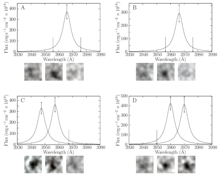
Figure 6: ELG candidates in the field of MRC B1256-243. For each object, the graph shows the flux recorded in, and the wavelength at, each etalon transmission band. The width of the curves indicate the etalon transmission profile. 14 pixel square thumbnail images are displayed of the objects as seen in each band.

Four candidate emission line galaxies were identified in the field of MRC B1256-243. Details are given in Table 3, and their locations are shown in Fig. 3(a). Thumbnail images of the candidate galaxies from each field, together with the measured fluxes, are shown in Fig. 6.

4.2 MRC B2158-206

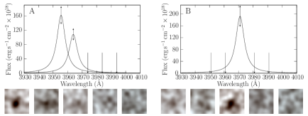
Figure 7: ELG candidates in the field of MRC B2158-206. For each object, the graph shows the flux recorded in, and the wavelength at, each etalon transmission band. The width of the curves indicate the etalon transmission profile. 14 pixel square thumbnail images are displayed of the objects as seen in each band.

Two candidate emission line galaxies were identified in the field of MRC B2158-206. Details are given in Table 3, and their locations are shown in Fig. 3(b). Thumbnail images of the candidate galaxies from each field, together with the measured fluxes, are shown in Fig. 7.

4.3 BR B0019-1522

Seventeen candidate emission line galaxies were identified in the field of BR B0019-1522. Details are given in Table 3, and their locations are shown in Fig. 3(c). Thumbnail images of the candidate galaxies from each field, together with the measured fluxes, are shown in Fig. 8.

4.4 Contaminants

This section briefly addresses the likelihood that our method might incorrectly identify another sort of object as an ELG.

4.4.1 Continuum objects

As per Figs. 1 and 2, the sensitivity of our instrument varies from image to image. Therefore, it is possible that a flat-spectrum continuum object may be detected in some images but not others, thereby appearing to be a potential ELG.

We use the results of Section 3 to estimate the probability of this occurring. Each of the 250,000 simulated objects was sorted into one of 3,600 bins by wavelength and magnitude (each bin covering 1 Å and 0.1 magnitudes). It is then possible to calculate the completeness of the bin (i.e. the fraction of simulated objects which were recovered). Each candidate ELG is assigned to a bin, and we then check the corresponding bins in adjacent images for completeness. A low completeness value in these bins indicates that a flat-spectrum object may have been ‘lost’.

This procedure calls into question four objects: A in the field of MRC B2158-206, B in the field of MRC B2156-243 and E and K in the field of BR B0019-1522. These sources were examined by eye, but there is no indication of a faint detection in the crucial frame. They have not, therefore, been excluded from this analysis.

4.4.2 Lower redshift interlopers

Another possibility is other emission lines at lower redshift may appear in our observations. The lines which might be observed are listed in Table 4.

Table 4: Potential low-redshift ‘interloper’ emission lines, together with the redshifts at which they appear and the estimated number observed in each of the fields. The flux of each line relative to H $\alpha$ in a “typical” galaxy is given, based on Kennicutt (1992).

Line	Å	Flux	MRC B2158-206		MRC B1256-243		BR B0019-1522
	(rest)	ratio	$z$	Number	$z$	Number	$z$	Number
$[$O ii$]$	3727	$0.41\pm 0.21$	0.065	∗0.05∗	0.060	0.02	0.803	1.93
H $\beta$	4860	$0.14\pm 0.06$	-	-	-	-	0.383	1.68
$[$O iii$]$	5007	$0.20\pm 0.15$	-	-	-	-	0.342	1.41
H $\alpha$	6548	$1.00\pm 0.00$	-	-	-	-	0.027	∗0.01∗
$[$N ii$]$	6583	$0.43\pm 0.16$	-	-	-	-	0.021	∗0.01∗

Cowie et al. (1997) and Gallego et al. (1995) provide number density counts for star forming galaxies at a range of redshifts. Both adopt a $H_{0}=50$ km s^-1 Mpc^-3, $\Omega_{\Lambda}=0$, $\Omega_{\mathrm{M}}=1$ cosmology, which we converted to match that used in this work (Section 1). In addition, Gallego et al. assume a Scalo (1986) IMF; Cowie et al. provide a conversion to a Salpeter (1955) IMF, and it is these results we adopt in this work. Based on these, we can estimate the number density of star forming galaxies along our line of sight: see Fig. 4.

Figure 4: Variation of galaxy number density with star formation rate for a range of redshifts. Based on data from Cowie et al. (1997) and Gallego et al. (1995).

Kennicutt (1998) provides a conversion between star formation rate in a galaxy and H $\alpha$ luminosity; the ratios given in Table 4 make it possible to convert that into expected luminiosities for the other lines. After applying a correction for instrumental effects and galactic extinction (Schlegel et al., 1998), a locus of points in the magnitude-wavelength completeness diagrams (Fig. 2) on which each line at a given redshift might be detected is determined. This locus is then integrated to estimate the total volume over which the line might be observed at this redshift. This procedure is then repeated along the full length of the curves shown in Fig. 4. In this way, the total number of interlopers which might be observed is estimated. The results are shown in Table 4.

It is clear that the estaimted number of interlopers is negligible in the case of the two lower-redshift fields. However, it is possible that as many as five of the candidate ELGs in the BR B0019-1522 field are, in fact, low redshift interlopers. This could only be confirmed by further observations.

5 Properties of candidate ELGs

In this section, we consider the distribution of candidate ELGs around the quasars to determine whether the quasar lies in an identifiable overdensity relative to the field.

The small number of candidates around the lower-$z$ quasars renders a meaningful statistical analysis of the individual fields unreliable. In an attempt to mitigate this, and given the apparent similarity of the fields, they are both considered as one unit in this section.

Figure 5: Distribution of ELG candidates around the quasars. On the left, the projected distance seen on the sky for both the ELG candidates (boxes) and all the objects observed (crosses); at right, the relative velocities.

The distribution of ELG candidates around the quasar is shown in both projection on the sky (left) and velocity distribution (right) in Fig. 5. When calculating the projection on the sky, we have normalised the total visible area on the sky in each distance bin. We also plot the distribution of all objects detected by SExtractor in the field for comparison.

Based on these figures, there is little evidence of projected clustering in the low-$z$ fields. However, there is a notably higher density of objects within 1 Mpc (projected) of BR B0019-1522. This is consistent with what one might expect from an examination of Fig. 3: note the large number of objects to the east of the quasar in Fig. 3(c). It is also in-line with the scale lengths observed in clusters around other AGN (Venemans et al., 2002; Bremer et al., 2002; Barr et al., 2004).

There is no suggestion of clustering in velocity space in Fig. 5. In part, this may be due to the low number of detections in the low-$z$ fields. In the field of BR B0019-1522, we note that all candidates were observed as bluer than the quasar itself; this is noteworthy, but not implausible given the wavelength range probed (6650–6740 Å, with the quasar at 6722 Å). Although the bluest velocity bins show a lower number of total counts, this can be attributed to the reduced instrumental sensitivity at the relevant wavelengths (see Fig. 3(c)).

The space density of galaxies in the three fields may also be estimated. As alluded to in the previous section, the comoving volume being probed by our measurements varies with wavelength and magnitude. Consider for example Fig. 2(a): a bright object–magnitude 19, say–may be detected at a range of wavelengths, from around 3920 Å to 4010 Å. A fainter object at, for instance, magnitude 22 is only detected if it lies within a much smaller wavelength range: around 3940 Å to 3960 Å. Therefore, we define an ‘accessible volume’, $\mathcal{V}_{n}$, for each detected object $n$ within the field. $\mathcal{V}_{n}$ is calculated by taking the locus of points in Fig. 2 occupied by a source with the observed properties and integrating over all wavelengths. The density is taken as $\rho=1/\mathcal{V}_{1}+1/\mathcal{V}_{2}+...+1/\mathcal{V}_{n}$. The results for our fields are given in Table 5.

Table 5: Estimated space and star formation rate densities, together with the total number of ELG candidates (#), for each of the fields observed. Note that our observations are valid only to an approximately defined lower limit of star formation.

Field	#	Number density	SFR density
		(Mpc${}^{-3}\,\times\,10^{4}$)	(M${}_{\odot}\;$ yr-1 Mpc-3)
MRC B1256	04	$22.48\pm 11.64$	$0.0346\pm 0.0174$
MRC B2158	02	$\phantom{0}9.09\pm\phantom{0}6.52$	$0.0070\pm 0.0049$
BR B0019	17	$49.09\pm 12.21$	$0.0484\pm 0.0117$

It is also instructive to estimate the star formation rates found in these fields. Based on Kennicutt et al. (1994) combined with Brocklehurst (1971) and Hu & McMahon (1996), we arrive at the relationship:

$$\mathrm{SFR}(\mathrm{M}_{\odot}\,\mathrm{yr^{-1}})=0.91\times 10^{-42}L(\mathrm{Ly}\alpha)(\mathrm{erg\,s^{-1}})$$ (5)

It should be noted that Ly $\alpha$ is a very poor indicator of star formation rate. It is resonantly scattered by neutral hydrogen, and hence has a high chance of absorption either before leaving the galaxy or by clouds in the intergalactic medium (Haiman & Spaans, 1999). Further, Valls-Gabaud (1993) argues that Ly $\alpha$ emission in starbursts is strongly dependent on the age of the burst, rendering the calibration of Equation 5 unreliable from around $10^{7}$ years after the burst start. Nevertheless, Ly $\alpha$ is the only diagnostic available to us, so we persist in these estimates with caution.

We take the star formation rate density as $\rho_{SFR}=SFR_{1}/\mathcal{V}_{1}+SFR_{2}/\mathcal{V}_{2}+...+SFR_{n}/\mathcal{V}_{n}$, where $SFR_{n}$ is the star formation rate associated with ELG candidate $n$ as calculated by Equation 5. Recall from Section 2.4 that the line fluxes are systematically underestimated since objects will fall outside the peaks of the etalon passpands. Making the approximation that objects are evenly spread in wavelength around the etalon peaks, we apply a correction to the observed magnitudes of 0.23 (in the low-$z$ field) or 0.27 (BR B0019-1522 field) to account for this. We correct the results for completeness based on Fig. 2: a single detection in an area with a low detection rate is taken as representative of a larger population.

The results are shown in Table 5. Note that our observations are sensitive to galaxies only down to some minimum level of star formation (9 M_⊙ yr^-1 in the case of MRC B2158-206 and BR B0019-1522; 25 M_⊙ yr^-1 in the case of MRC B1256-243): there may be a fainter population which we do not probe.

It is noteworthy that the star formation rate in the field of MRC B1256-243 is anomalously high, but the large uncertainties in the field and the higher minimum detectable rate render this result questionable. The most well constrained result is that for BR B0019-1522; our results there are broadly similar to those reported by Venemans et al. (2002) around the $z=4.1$ radio galaxy TN J1338-1942. In all three fields, the number of objects detected is higher than that which might be expected in the absence of any clustering. Based on Cowie et al. (1997), we might expect on average 0.86 galaxies in the field of MRC B2158-206, 0.25 in that of MRC B1256-243, and 1.3 in that of BR B0019-1522, while an extrapolation from the results of the LALA (‘Large Area Lyman $\alpha$’; Rhoads et al., 2000) survey suggests we should observe 1.1 objects in the field of MRC B2158-206, 0.8 in that of MRC B1256-243 and 2.1 in that of BR B0019-1522 (assuming that the density of Ly $\alpha$ emitters is similar at $z\sim 2.2$ to that observed at $z\sim 4.5$).

6 Conclusions

Until recently, it has proved difficult to find high-redshift clusters and, indeed, there are very few known beyond $z\sim 1$. The detection of hot X-ray emission from intracluster gas followed by optical imaging and/or spectroscopic confirmation becomes inefficient for detecting more distant clusters; a manifestly higher success rate is achieved by targeting the vicinity of high redshift radio galaxies and quasars.

We have used tunable filter observations to identify a galaxy overdensity in the field of BR B0019-1522, with a local number density an order of magnitude higher than that which might be expected in the field. This is among the highest-redshift clusters detected around a radio quiet quasar. We have also identified potential overdensities in the fields of and MRC B1256-243 and MRC B2158-208, although deeper observations are required to confirm these detections.

The current observations were made with the Taurus Tunable Filter, an instrument which has now been decommissioned, on the 4 metre class Anglo-Australian Telescope. These observations have clearly demonstrated the success of the tunable imaging technique. The prospects for further progress in this area are strong, as the next generation of tunable filter instruments are now available or becoming available on telescopes such as the GTC 10-m (OSIRIS; Cepa et al., 2000), SOAR 4-m (BTFI; Taylor et al., 2010), SALT 11-m (PFIS; Smith et al., 2006), NTT 3.5-m (3D-NTT; Marcelin et al., 2008) and the Magellan 6.5-m (MMTF; Veilleux et al., 2010).

With existing telescopes, it is very difficult to extract more information than a few emission lines and broadband photometry for the host galaxies in these high-redshift environments. More detailed spectral information will not be possible until the next generation of extremely large telescopes or the James Webb Space Telescope come on line. But there are other uses for these observations: in particular, Bruns et al. (2011) have shown that quasar environments may act as a surrogate for studying the radiative suppression of galaxy formation during the epoch of reionization. Interestingly, the UV suppression reduces the star-forming galaxy counts by a factor of 2–3 but does not suppress them altogether. The time is therefore ripe to further develop this promising method of investigation in order to learn about the occurrence of high-redshift, star forming groups and the impact on these groups by quasar activity.

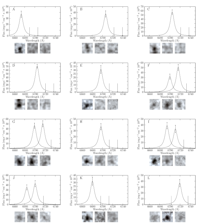
Figure 8: ELG candidates in the field of BR B0019-1522. For each object, the graph shows the flux recorded in, and the wavelength at, each etalon transmission band. The width of the curves indicate the etalon transmission profile. 14 pixel square thumbnail images are displayed of the objects as seen in each band.

Figure 8 (contd). ELG candidates in the field of BR B0019-1522.

References

- Bahcall et al. (1969) Bahcall J. N., Schmidt M., Gunn J. E., 1969, ApJ, 157, L77
- Baker et al. (2001) Baker J. C., et al., 2001, AJ, 121, 1821
- Barr et al. (2004) Barr J., Baker J., Bremer M., Hunstead R., Bland-Hawthorn J., 2004, AJ, 121, 2660
- Bertin & Arnouts (1996) Bertin E., Arnouts S., 1996, A&AS, 117, 393
- Bland & Tully (1989) Bland J., Tully R. B., 1989, AJ, 98, 723
- Bland-Hawthorn & Jones (1998) Bland-Hawthorn J., Jones D. H., 1998, Publications of the Astronomical Society of Australia, 15, 44
- Bremer & Baker (1999) Bremer M. N., Baker J. C., 1999, in Röttgering H. J. A., Best P. N., Lehnert M. D., eds, The Most Distant Radio Galaxies Radio-loud quasars in distant groups and clusters. Royal Netherlands Academy of Arts and Sciences, pp 425–436
- Bremer et al. (2002) Bremer M. N., Baker J. C., Lehnert M. D., 2002, MNRAS, 337, 470
- Brocklehurst (1971) Brocklehurst M., 1971, MNRAS, 153, 471
- Bruns et al. (2011) Bruns Jr. L. R., Wyithe J. S. B., Bland-Hawthorn J., Dijkstra M., 2011, ArXiv e-prints
- Cepa et al. (2000) Cepa J., et al., 2000, in Iye M., Moorwood A. F., eds, Optical and IR telescope instrumentation and detectors Vol. 4008 of SPIE Conf. Ser. pp 623–631
- Cowie et al. (1997) Cowie L. L., Hu E. M., Songaila A., Egami E., 1997, ApJ, 481, L9
- Dawson et al. (2004) Dawson S., et al., 2004, ApJ, 617, 707
- Francis & Bland-Hawthorn (2004) Francis P. J., Bland-Hawthorn J., 2004, MNRAS, 353, 301
- Gallego et al. (1995) Gallego J., Zamorano J., Aragon-Salamanca A., Rego M., 1995, ApJ, 455, L1
- Haiman & Spaans (1999) Haiman Z., Spaans M., 1999, ApJ, 518, 138
- Hamuy et al. (1992) Hamuy M., Walker A., Suntzeff N., Gigoux P., Heathcote S., Phillips M., 1992, PASP, 104, 533
- Hu & McMahon (1996) Hu E. M., McMahon R. G., 1996, Nat, 382, 231
- Jones & Bland-Hawthorn (2001) Jones D. H., Bland-Hawthorn J., 2001, ApJ, 550, 593
- Jones et al. (2002) Jones D. H., Shopbell P. L., Bland-Hawthorn J., 2002, MNRAS, 329, 759
- Kaiser (1991) Kaiser N., 1991, ApJ, 383, 104
- Kapahi et al. (1998) Kapahi V., et al., 1998, ApJS, 118, 327
- Kennicutt (1998) Kennicutt R. C., 1998, ARA&A, 36, 189
- Kennicutt et al. (1994) Kennicutt R. C., Tamblyn P., Congdon C. E., 1994, ApJ, 435, 22
- Kennicutt (1992) Kennicutt Jr. R. C., 1992, ApJ, 388, 310
- Kuiper et al. (2011) Kuiper E., et al., 2011, ArXiv e-prints
- Kurk et al. (2000) Kurk J. D., et al., 2000, A&A, 358, L1
- Le Delliou et al. (2006) Le Delliou M., Lacey C. G., Baugh C. M., Morris S. L., 2006, MNRAS, 365, 712
- McLure & Dunlop (2001) McLure R. J., Dunlop J. S., 2001, MNRAS, 321, 515
- Marcelin et al. (2008) Marcelin M., et al., 2008, in McLean I. S., Casali M. M., eds, Ground-based and Airborne Instrumentation for Astronomy II Vol. 7014 of SPIE Conf. Ser. pp 701455–701455–8
- Oemler et al. (1972) Oemler A. J., Gunn J. E., Oke J. B., 1972, ApJ, 176, L47
- Oke (1974) Oke J. B., 1974, ApJS, 27, 21
- Overzier et al. (2006) Overzier R. A., et al., 2006, ApJ, 637, 58
- Pentericci et al. (2000) Pentericci L., et al., 2000, A&A, 361, L25
- Rawlings & Jarvis (2004) Rawlings S., Jarvis M. J., 2004, MNRAS, 355, L9
- Rhoads et al. (2000) Rhoads J. E., Malhotra S., Dey A., Stern D., Spinrad H., Jannuzi B. T., 2000, ApJ, 545, L85
- Salpeter (1955) Salpeter E. E., 1955, ApJ, 121, 161
- Scalo (1986) Scalo J. M., 1986, Fundamentals of Cosmic Physics, 11, 1
- Schlegel et al. (1998) Schlegel D. J., Finkbeiner D. P., Davis M., 1998, ApJ, 500, 525
- Smith et al. (2006) Smith M. P., et al., 2006, in McLean I. S., Iye M., eds, Ground-based and Airborne Instrumentation for Astronomy Vol. 6269 of SPIE Conf. Ser. p. 62692A
- Springel et al. (2005) Springel V., et al., 2005, Nat, 435, 629
- Stiavelli et al. (2005) Stiavelli M., et al., 2005, ApJ, 622, L1
- Tapken et al. (2004) Tapken C., et al., 2004, A&A, 416, L1
- Taylor et al. (2010) Taylor K., et al., 2010, in Atad-Ettedgui E., Lemke D., eds, Modern Technologies in Space- and Ground-based Telescopes and Instrumentation Vol. 7739 of SPIE Conf. Ser. pp 77394U–77394U–7
- Valls-Gabaud (1993) Valls-Gabaud D., 1993, ApJ, 419, 7
- Veilleux et al. (2010) Veilleux S., et al., 2010, AJ, 139, 145
- Venemans et al. (2002) Venemans B. P., et al., 2002, ApJ, 569, L11
- Venemans et al. (2004) Venemans B. P., et al., 2004, A&A, 424, L17
- Venemans et al. (2005) Venemans B. P., et al., 2005, A&A, 431, 793