Grand Unification without Higgs Bosons

Abstract

We discuss how a model for the electroweak interactions without a Higgs could be embedded into a grand unified theory. The requirement of a non-trivial fixed point in the $SU(2)$ sector of the weak interactions together with the requirement of the numerical unification of the gauge couplings leads to a prediction for the value of the $SU(2)$ gauge coupling in the fixed point regime. The fixed point regime must be in the TeV region to solve the unitarity problem in the elastic scattering of W bosons. We find that the unification scale is at about $10^{14}$ GeV. Viable grand unified theories must thus conserve baryon number. We discuss how to build such a model without using Higgs bosons.

This paper is dedicated to the memory of Julius Wess. While Julius was a mathematical physicist, he truly had an amazing physical intuition and understanding for experimental developments. He was very much interested in seeing how his ideas could be applied to particle physics. It turns out that several of his mathematical constructions can be used to build elegant extensions of the standard model of particle physics. The most well known example is that of supersymmetry which is one of the most popular framework to address the fine tuning problem of the Higgs boson’s mass in the standard model. This article will be dealing with another potential extension of the standard model, without a Higgs boson this time, using techniques developed in the 1960’s by Callan, Coleman, Wess and Zumino [1] who understood that gauge symmetries could be implemented in a non-linear way. Nowadays, these models are called non-linear sigma models and have found beautiful applications in low energy QCD or in models of physics beyond the standard model with a composite Higgs boson.

Despite strong evidence for the existence of a standard model Higgs coming from ATLAS and CMS at the Large Hadron Collider, it is worthwhile to entertain the possibility that there is no fundamental Higgs boson as experimental data is not conclusive yet and the about 3 $\sigma$ signal for a 125 GeV Higgs boson could turn out to be a rather large background fluctuation. Also from a purely academic point of view, one can ask how one would build a Grand Unified Theory without fundamental scalars. We shall first review briefly how to build the standard model without a propagating Higgs boson [2, 3] and then extend these ideas to grand unified theories.

While the Higgs mechanism is an elegant tool to generate masses for the electroweak gauge bosons while preserving the perturbative unitarity of the S-matrix and the renormalizability of the theory, it is well understood that gauge symmetries can be implemented in a non-linear way [1]. We shall emphasize that mass terms for the electroweak bosons can be written in a gauge invariant way using a non-linear sigma model representation. We start with the Lagrangian

$$L_{SM}=L_{0}+L_{mass}$$ (1)

where

$$L_{0}=-\frac{1}{4}W^{a}_{\mu\nu}W^{a\,\mu\nu}-\frac{1}{4}B_{\mu\nu}B^{\mu\nu}-\frac{1}{4}G_{\mu\nu}G^{\mu\nu}+\sum_{j=1}^{3}\,\bar{\Psi}^{(j)}i\mathchoice{\ooalign{$\hfil\displaystyle\mkern 0.0mu/\hfil$\crcr$\displaystyle D$}}{\ooalign{$\hfil\textstyle\mkern 0.0mu/\hfil$\crcr$\textstyle D$}}{\ooalign{$\hfil\scriptstyle\mkern 0.0mu/\hfil$\crcr$\scriptstyle D$}}{\ooalign{$\hfil\scriptscriptstyle\mkern 0.0mu/\hfil$\crcr$\scriptscriptstyle D$}}\Psi^{(j)}$$ (10)

and

$$L_{mass} = M_{W}^{2}\,W^{+}_{\mu}W^{-\,\mu}+\frac{1}{2}M_{Z}^{2}\,Z^{\mu}Z_{\mu}$$

$$\qquad\qquad-\sum_{i,j}\Big{(}\bar{u}^{(i)}_{L}M^{u}_{ij}u_{R}^{(j)}+\bar{d}^{(i)}_{L}M^{d}_{ij}d_{R}^{(j)}+\bar{e}^{(i)}_{L}M^{e}_{ij}e_{R}^{(j)}+\bar{\nu}^{(i)}_{L}M^{\nu}_{ij}\nu_{R}^{(j)}\Big{)}+h.c.\,,$$

where $\Psi=\{q^{i}_{L},u^{i}_{R},d^{i}_{R},l^{i}_{L},e^{i}_{R},\nu^{i}_{R}\}$ stands for the standard model fermions and $i,j$ are generation indices. The mass terms for the gauge bosons and fermions above arise from the manifestly gauge invariant Lagrangian

$$L_{mass}=\frac{v^{2}}{4}\text{Tr}\left[\left(D_{\mu}\Sigma\right)^{\dagger}\left(D^{\mu}\Sigma\right)\right]-\frac{v}{\sqrt{2}}\sum_{i,j}\left(\bar{u}_{L}^{(i)}d_{L}^{(i)}\right)\Sigma\begin{pmatrix}\lambda_{ij}^{u}\,u_{R}^{(j)}\\[2.84544pt] \lambda_{ij}^{d}\,d_{R}^{(j)}\end{pmatrix}+h.c.$$ (12)

The field $\Sigma(x)$ is given by

$$\Sigma(x)=\exp(i\sigma^{a}\chi^{a}(x)/v)$$ (13)

where $\chi_{a}$ are the Goldstone bosons of $SU(2)_{L}$ and the covariant derivative by

$$D_{\mu}\Sigma=\partial_{\mu}\Sigma-ig\frac{\sigma^{a}}{2}W^{a}_{\mu}\Sigma+ig^{\prime}\Sigma\frac{\sigma^{3}}{2}{\cal A}_{\mu}\,.$$ (14)

The local $SU(2)_{L}\times U(1)_{Y}$ invariance is evident, since $\Sigma$ transforms as

$$\Sigma\rightarrow U_{L}(x)\,\Sigma\,U_{Y}^{\dagger}(x)$$ (15)

with

$$U_{L}(x)=\exp\big{(}i\alpha_{L}^{a}(x)\sigma^{a}/2\big{)}\ \mbox{and}\ U_{Y}(x)=\exp\big{(}i\alpha_{Y}(x)\sigma^{3}/2\big{)}.$$ (16)

The fields $\chi^{a}$ are transforming in a non-linear way under a local $SU(2)_{L}\times U(1)_{Y}$ gauge transformations

$$\chi^{a}(x)\rightarrow\chi^{a}(x)+\frac{v}{2}\,\alpha_{L}^{a}(x)-\frac{v}{2}\,\delta^{a3}\,\alpha_{Y}(x)\,.$$ (17)

In the unitary gauge, $\langle\Sigma\rangle=1$, the chiral Lagrangian (12) reproduces the mass term of Eq.(1) with

$$\rho\equiv\frac{M_{W}^{2}}{M_{Z}^{2}\cos^{2}\theta_{W}}=1\,.$$ (18)

This relation is consistent with the experimentally measured value to quite good accuracy. It follows as the consequence of the approximate invariance of (12) under $SU(2)_{L}\times SU(2)_{R}$ global transformations,

$$\Sigma\rightarrow U_{L}\,\Sigma\,U_{R}^{\dagger}\,,$$ (19)

which is spontaneously broken to the diagonal subgroup $SU(2)_{c}$ by $\langle\Sigma\rangle=1$, and explicitly broken by $g^{\prime}\not=0$ and $\lambda^{u}_{ij}\not=\lambda^{d}_{ij}$. In the limit of vanishing $g^{\prime}$ the fields $\chi^{a}$ transform as a triplet under the “custodial” $SU(2)_{c}$, so that $M_{W}=M_{Z}$.

This formulation is mathematically identical to the one presented in terms of gauge invariant fields in [3]. The electroweak bosons can be defined in terms of gauge invariant fields given by

$$\underline{W}^{i}_{\mu} = \frac{i}{2g}\mbox{Tr}\ \Omega^{\dagger}\stackrel{{\scriptstyle\leftrightarrow}}{{D_{\mu}}}\Omega\tau^{i}$$ (20)

with $D_{\mu}=\partial_{\mu}-ig\frac{\sigma_{a}}{2}B^{a}_{\mu}(x)$ and

$$\Omega=\frac{1}{\sqrt{\phi^{\dagger}\phi}}\left(\begin{array}[]{cc}\phi_{2}^{*}&\phi_{1}\\ -\phi_{1}^{*}&\phi_{2}\end{array}\right)$$ (23)

where

$$\phi=\left(\begin{array}[]{c}\phi_{1}\\ \phi_{2}\end{array}\right).$$ (26)

is a $SU(2)_{L}$ doublet scalar field which is considered to be a dressing field and does not need to propagate. The very same construction can be applied to fermions [3, 4, 5, 6, 7]:

$$\underline{\psi}^{a}_{L} = \Omega^{\dagger}\psi^{a}_{L}$$ (27)

where $\psi^{a}_{L}$ are the usual $SU(2)_{L}$ doublets.

Now clearly the standard model without a propagating Higgs boson is not renormalizable at the perturbative level. In fact, an infinite number of higher dimensional operators will be generated by radiation corrections:

$$S=S_{SMw/oHiggs}+\int d^{4}x\sum_{i}\frac{C_{i}}{v^{n}}O^{4+n}_{i}$$ (28)

where $O^{4+n}_{i}$ are operators compatible with the symmetries of the model. There is a beautiful analogy between this theory and quantum general relativity

$$S[g]=-\int d^{4}x\sqrt{-\det(g)}\!\!\!\!\! \left(-\Lambda(\mu)+\frac{\bar{M}_{P}^{2}(\mu)}{32\pi}R+a(\mu)R_{\mu\nu}R^{\mu\nu}+b(\mu)R^{2}\right.$$

$$\left.+\frac{c(\mu)}{\bar{M}_{P}^{2}}R^{3}+\frac{d(\mu)}{\bar{M}_{P}^{2}}RR_{\mu\nu}R^{\mu\nu}+....\right).$$

While quantum general relativity is not renormalizable at the perturbative level as well, Weinberg [8] argued some 40 years ago that it might be renormalizable at the non perturbative level if there is a non-trivial fixed point. Evidence for the existence of such a non -trivial fixed point has accumulated over the last 40 years. This approach is known as asymptotic safety. While calculations to identify such fixed points are difficult and often involve uncontrolled approximation, this approach to quantum gravity is clearly very exciting as it is very conservative and does not require new speculative theories to formulate quantum gravity.

If there is no propagating Higgs boson, it is most natural to posit that the weak interactions are asymptotically safe. This implies the existence of non-trivial fixed points in the $SU(2)_{L}$ gauge interactions and Yukawa sectors. Amazingly, there are indeed indications of a non-trivial fixed point in non linear sigma models [9, 10, 11]. It should be stressed nevertheless that these indications rely on a truncation of the effective action which can be considered as an uncontrolled approximation. However, while in the case of gravity it might never possible to observe the fixed point regime, we expect that this will be the case at the LHC for the weak interactions, if this mechanism has been chosen by nature.

Besides a non-trivial fixed point, the weak scale must have a non-trivial running to suppress the growth of the W-W scattering amplitude with energy. Formally, one can introduce a dimensionless coupling constant:

$$g_{v}=k^{2}/v(k)^{2}$$ (30)

where $k$ is the renormalization group momentum scale. A renormalization group equation for $g_{v}$ can be written as

$$\frac{\partial g_{v}}{\partial\ln k}=\beta_{k}=(d-2+\eta)g_{v}$$ (31)

where $d$ is the number of dimensions and with the anomalous dimension of the weak bosons given by

$$\eta=-\frac{\partial\ln Z(k)}{\partial\ln k}$$ (32)

which in general is a function of all the couplings of the Lagrangian (28). $Z(k)$ denotes the wave-function renormalisation factor of the electroweak bosons. In four dimensions, there is a non-trivial fixed point if $\eta=-2$. In analogy to the non-perturbative running of the non-perturbative Planck mass, we introduce an effective weak scale

$$v_{eff}^{2}=v^{2}\left(1+\frac{\omega}{8\pi}\frac{\mu^{2}}{v^{2}}\right)$$ (33)

where $\mu$ is some arbitrary mass scale, $\omega$ a non-perturbative parameter which determines the running of the effective weak scale and $v$ is the weak scale measured at low energies. If $\omega$ is positive, the electroweak interactions would become weaker with increasing center of mass energy. Suppressing the growth of the partial wave amplitude enough to maintain the unitarity bound at all scales requires $\omega\geq 1/3$.

While the model formulated above represents a perfectly natural and consistent ultraviolet completion of the standard model, it is natural to wonder whether grand unification is compatible with that framework. Grand unified theories are fascinating models and the realization that the fermions of the standard model fit naturally into representations of simple groups such as $SU(5)$ or $SO(10)$ is a strong motivation to consider these ideas. As always, the messy part comes with the spontaneous symmetry breaking of these large group to that of the standard model. Realistic models require the inclusion of many new Higgs bosons which has always led to theoretical problems such as the hierarchy problem, the doublet-triplet mass-splitting problem, and higher dimensional operators involving the Higgs bosons which can lead to sizable threshold effects which are very difficult to evaluate. It is thus tempting to build grand unified theories without Higgs bosons while preserving the beautiful aspects of grand unification.

The requirement of the numerical unification of the coupling of the standard model without a Higgs boson leads to an interesting prediction for the value of the $SU(2)$ gauge coupling in the fixed point regime. If there is a non-trivial fixed point, the beta function of the $SU(2)_{L}$ is zero and the coupling constant is thus fixed. The beta functions of the $U(1)$ and $SU(3)$ are given by their usual Standard Model values with the caveat that there are no scalars and the value of the $U(1)$ beta function in our model will thus differ from that of the standard model. We have

$$\mu\frac{\partial}{\partial\mu}\alpha_{i}(\mu)=\frac{1}{2\pi}b_{i}\alpha_{i}^{2}(\mu)$$ (34)

with

$$b^{UV}_{i}=\left(\begin{array}[]{c}b_{1}\\ b_{2}\\ b_{3}\end{array}\right)=\left(\begin{array}[]{c}0\\ 0\\ -11\end{array}\right)+N_{gen}\left(\begin{array}[]{c}4/3\\ 0\\ 4/3\end{array}\right)$$ (44)

we assume that the number of generations $N_{gen}=3$. Requiring that the $U(1)$ and $SU(3)$ gauge coupling meet in one point allow us to determine the unified coupling constant and the unification scale. We find that the unified coupling constant is $\alpha_{\star}=1/40.6$ and the unification scale $\mu_{\star}=3.2\times 10^{14}$ GeV. This allows us to determine the value of the coupling constant in the fixed point domain which is identical to the unified coupling constant. This is a prediction of this unification mechanism. Our result is illustrated in Fig. (1). We assumed that the fixed point is in the TeV region. This is necessary to suppress the growth of the W-W scattering amplitude. Below that scale we used the usual standard model value for the beta function of the $SU(2)$ however without a Higgs doublet, i.e. $b_{2}=-22/3+N_{gen}4/3$.

Note that in Fig. (1), we assume that the running of the $SU(2)_{L}$ coupling constant is given by the standard model equation without a Higgs boson and replaced by the fixed-point value above a TeV. This approximation is similar to what is done in supersymmetric models where it is assumed that the superpartners do not contribute below one TeV, while they do above the energy scale above which supersymmetry is restore. In our case, we expect the running to be more complicated than this close to the fixed-point. We expect that the $SU(2)_{L}$ coupling constant will increase, hence making the higher dimensional operators discussed above more important before reaching its constant value in the fixed-point region. We stress that our approximation is not important for our numerical evaluation.

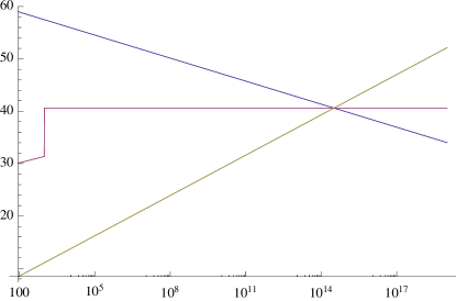
Figure 1: This is a logarithmic plot of $\alpha_{i}^{-1}$ as a function of the running scale $\mu$.

An obvious issue is that if we use conventional grand unified theories such as $SU(5)$[12] or $SO(10)$[13], there are dimension six operators which lead to a proton decay rate which is excluded by current observations. We are thus forced to consider grand unified theories which do not have proton decay. Fortunately, such models do exist [14, 15]. The reason for proton decay in most grand unified models is that leptons and quarks are unified in the same multiplets of the grand unified theory. For example, in $SU(5)$ they are unified in the $\bar{5}$ and $10$, the heavy gauge bosons $X$ and $Y$ of $SU(5)$ with masses of the order of the unification scale lead to a fast decay of the proton. There are several possibilities to suppress proton decay if the model is formulated in higher dimensions [14, 15] (see also [16, 17] for older GUT models with a stable proton). In four dimensions one can rely on more complicated unified structures such as $SU(3)^{3}$ trinification or $SU(N)\times SU(N)$ which typically do not have $X$ and $Y$ gauge bosons and thus no gauge-mediated proton decay if the matter representations are chosen appropriately. While in conventional models with a Higgs mechanism there can still be proton decay mediated by colored Higgs bosons, we would not have such a problem with our approach where the Higgs bosons are replaced by non linear sigma models.

It is also possible to have models with simple groups [14], for example a $SU(5)$ grand unified theory with an unusual fermion assignment. The authors of [14], for example, suggest taking states $\bar{F}_{1,2}\sim\bar{5}$ and $T_{1,2,3}\sim 10$ and anti-states $F$ and $\bar{T}_{1,2}$ per generation. The $SU(5)$ symmetry is broken by the fields $\Phi$ and $\Omega$, both in the reducible 24+1 representations, having the following vacuum expectations: $\langle\Phi\rangle=v_{1}\mbox{diag}(1,1,1,0,0)$ and $\langle\Omega\rangle=v_{2}\mbox{diag}(0,0,0,1,1)$ for which in our approach we represent by non linear sigma models. They also introduce one extra 24 + 1 field $\Sigma$ which develops a vacuum expectation value of the form $\langle\Sigma\rangle=\sigma\mbox{diag}(1,1,1,-1,-1)$. A Yukawa interaction

$$(\bar{F}_{1}F+T_{1}\bar{T}_{1})\Phi+(\bar{F}_{2}F+T_{2}\bar{T}_{1})\Omega+T_{3}\bar{T}_{2}\Sigma$$ (45)

where $\Phi$, $\Omega$ and $\Sigma$, in our approach, are non-linear sigma models will give masses to the heavy fermions, the light fermions of the standard model can be identified as in [14]: $L\subset\bar{F}_{1}$, $d^{c}\subset\bar{F}_{2}$, $e^{c}\subset T_{1}$, $u^{c}\subset T_{2}$ and $Q\subset T_{3}$. This assignment insures that lepton and baryon numbers are preserved to all orders in perturbation theory.

In conclusion, we have discussed how a model for the electroweak interactions without a Higgs could be embedded into a grand unified theory. The requirement of a non-trivial fixed point in the $SU(2)$ sector of the weak interactions together with the requirement of the numerical unification of the gauge couplings leads to a prediction for the value of the $SU(2)$ gauge coupling in the fixed point regime. The fixed point regime must be in the TeV region to solve the unitarity problem in the elastic scattering of W bosons. We find that the unification scale is at about $10^{14}$ GeV. Viable grand unified theories must thus conserve baryon number. We have discussed how to build such a model without using Higgs bosons.

References

- [1] C. G. Callan, S. R. Coleman, J. Wess and B. Zumino, Phys. Rev. 177, 2247 (1969).
- [2] X. Calmet, Mod. Phys. Lett. A26, 1571-1576 (2011). [arXiv:1012.5529 [hep-ph]].
- [3] X. Calmet, Int. J. Mod. Phys. A26, 2855-2864 (2011). [arXiv:1008.3780 [hep-ph]].
- [4] G. ’t Hooft, “Topological aspects of quantum chromodynamics”, Lectures given at International School of Nuclear Physics: 20th Course: Heavy Ion Collisions from Nuclear to Quark Matter (Erice 98), Erice, Italy, 17-25 Sep 1998, “Topological aspects of quantum chromodynamics,” hep-th/9812204, published in “Erice 1998, From the Planck length to the Hubble radius,” 216-236.
- [5] G. ’t Hooft, in “Recent Developments In Gauge Theories,” Cargèse 1979, ed. G. ’t Hooft et al. Plenum Press, New York, 1980, Lecture II, p.117, “Recent Developments In Gauge Theories. Proceedings, Nato Advanced Study Institute, Cargèse, France, August 26 - September 8, 1979.”
- [6] G. Mack, “Quark And Color Confinement Through Dynamical Higgs Mechanism,” DESY-77-58.
- [7] V. Visnjic, Nuovo Cim. A 101, 385 (1989).
- [8] S. Weinberg, in Understanding the Fundamental Constituents of Matter, ed. A. Zichichi (Plenum Press, New York, 1977); in General Relativity, ed. S. W. Hawking and W. Israel (Cambridge University Press, 1979): 700.
- [9] M. Fabbrichesi, R. Percacci, A. Tonero and O. Zanusso, arXiv:1010.0912 [hep-ph].
- [10] R. Percacci, arXiv:0910.4951 [hep-th].
- [11] R. Percacci and O. Zanusso, Phys. Rev. D 81, 065012 (2010) [arXiv:0910.0851 [hep-th]].
- [12] H. Georgi and S. L. Glashow, Phys. Rev. Lett. 32, 438 (1974).
- [13] H. Fritzsch and P. Minkowski, Annals Phys. 93, 193 (1975).
- [14] Z. Berezhiani, I. Gogoladze and A. Kobakhidze, Phys. Lett. B 522, 107 (2001) [hep-ph/0104288].
- [15] A. B. Kobakhidze, Phys. Lett. B 514, 131 (2001) [hep-ph/0102323].
- [16] P. Langacker, G. Segre and H. A. Weldon, Phys. Lett. B 73, 87 (1978).
- [17] P. Langacker, G. Segre and H. A. Weldon, Phys. Rev. D 18, 552 (1978).