Statistical estimation of mechanical parameters of clarinet reeds using experimental and numerical approaches

Abstract

A set of 55 clarinet reeds is observed by holography, collecting 2 series of measurements made under 2 different moisture contents, from which the resonance frequencies of the 15 first modes are deduced. A statistical analysis of the results reveals good correlations, but also significant differences between both series. Within a given series, flexural modes are not strongly correlated. A Principal Component Analysis (PCA) shows that the measurements of each series can be described with 3 factors capturing more than $90\%$ of the variance: the first is linked with transverse modes, the second with flexural modes of high order and the third with the first flexural mode. A forth factor is necessary to take into account the individual sensitivity to moisture content. Numerical 3D simulations are conducted by Finite Element Method, based on a given reed shape and an orthotropic model. A sensitivity analysis revels that, besides the density, the theoretical frequencies depend mainly on 2 parameters: $E_{L}$ and $G_{LT}$. An approximate analytical formula is proposed to calculate the resonance frequencies as a function of these 2 parameters. The discrepancy between the observed frequencies and those calculated with the analytical formula suggests that the elastic moduli of the measured reeds are frequency dependent. A viscoelastic model is then developed, whose parameters are computed as a linear combination from 4 orthogonal components, using a standard least squares fitting procedure and leading to an objective characterization of the material properties of the cane Arundo donax.

1 Introduction

Clarinettists experience every day the crucial importance of clarinet reeds for the quality of sound. Their characterization is a real challenge for musicians who wish to obtain reeds that are suited to their personal needs. The present paper address this complex field of research. Its scope is restricted to the development of an objective method for a mechanical characterization of single reeds of clarinet type. >From the shape and the resonance frequencies of each individual reed (measured with heterodyne holography), we intend to deduce the mechanical properties of the material composing it. A subsequent study should then examine how these mechanical properties are correlated with the musical properties of the reeds.

Generally, the physicist chooses a model in order to validate it by observations. In the present study, the complexity of the problematic forced us to adopt the reverse attitude: We observe the mechanical behavior of clarinet reeds with a statistically representative sample and exploit afterward the statistical results for establishing a satisfactory mechanical model designed with a minimal number of parameters.

Natural materials, as wood or cane, are often orthotropic and exhibit a different stiffness along the grain (longitudinally) as in the others directions. The problem is then obviously multidimensional. Nevertheless, reed makers classify their reeds by a single parameter: the nominal reed "strength" (also called "hardness"), in general from 1 to 5, which basically reflects the stiffness of the material (cane, Arundo donax L.), since all reeds of the same model have theoretically the same shape. The method of measurement is generally not publicized by manufacturers, but this "strength" is probably related to the static Young modulus in the longitudinal direction $E_{L}$.

"Static" (i.e. low frequency) measurements of the elastic parameters of cane are available in the literature, for instance Spatz et al. [1]. A viscoelastic behavior has been reported in experimental situations (see e.g. Marandas et al. [2], Ollivier [3] or Dalmont et al. [4]) and this fact seems generally well accepted in wood sciences and biomechanics (for instance Speck et al. [5, 6]). Marandas et al. proposed a viscoplastic model of the wet reed. Viscoelastic behavior for cane was already demonstrated by Chevaux [7], Obataya et al. [8, 9, 10, 11] and Lord [12]. These authors study only the viscoelasticity of the longitudinal Young modulus $E_{L}$, leaving aside the case of the shear modulus in the longitudinal/tangential plane $G_{LT}$. Furthermore, they give no really representative statistics about the variability of the measured parameters.

The observation of mechanical resonance frequencies can be achieved by different methods. The methods used by Chevaux, Obataya and Lord are destructive for the reed, which cannot be used for further musical tests. On the contrary, holography is a convenient non-destructive method, the reed being excited by a loudspeaker. For instance Pinard et al. [13] measured with this method the frequency of the 4 lowest resonances and focused their attention on the musical properties of the reeds.

The digital Fresnel holography method was used by Picart et al. [14, 15] and Mounier et al. [16] to measure high amplitude motion of a reed blown by an artificial mouth. Guimezanes [17] used a scanning vibrometer.

Recent technological developments provide very efficient and convenient measurements with holography, without having to manually identify the modes of resonance and to be satisfied with a single picture of their vibration: in a few minutes hundreds of holograms are acquired showing the response of a reed for many frequencies. The temperature and the moisture content can be considered as constant during a measurement series. The Sideband Digital Holography technique provides additional facilities (see 2.1.1).

Different authors (among them Casadonte [18, 19], Facchinetti et al. [20, 21] and Guimezanes [17]) modeled the clarinet reed by Finite Elements Method (FEM) and computed the first few eigenmodes. They chose appropriated values of the elastic parameters in the literature, ignoring however viscoelastic behavior. The goodness of fit between observations and model was of secondary importance, except for Guimezanes. This latter author built a 2-D elastic model of the reed with longitudinally varying parameters. He fitted his model quite adequately with his observations (only 5 resonances were measured), but the fitted parameters seem not really plausible physically. His model didn’t respect the assumption of a radial monotonically decrease of stiffness from the outer side to the inner side of the cane. Under such conditions, the frequency of the first resonance would increase in comparison to homogeneous material, and not decreased, as observed experimentally.

In Section 2 the measurement method is presented. The experimental setup is described in Section 2.1 and the method for observing resonance frequencies is detailed in 2.2. The results for 55 reeds are given in Section 3 (statistics, Principal Component Analysis (PCA)[22]).

In Section 4, the development and the selection of a satisfactory mechanical model with minimal structure is described. First, a numerical analysis of the resonance frequencies of a reed assumed to be perfectly elastic is done by Finite Element Method (FEM), and a metamodel computing the resonance frequencies from elastic parameters is given in Section 4.3. This allows solving the inverse problem in a fast way. However, because the elastic model is not very satisfactory, viscoelasticity has to be introduced and some parameters are added to the model in Section 4.4. The viscoelastic model has however too many degrees of freedom, according to PCA. Consequently, the viscoelastic parameters of the model are assumed to be correlated and PCA indicates that these parameters can be probably reconstructed from 4 orthogonal components, as a linear combination, by multiple regression (Section 5). The relationships between the components and the viscoelastic parameters is given, and finally the resulting values for these parameters are discussed in Section 5.3 and compared with the results of the literature.

2 Observations by Sideband Digital Holography

2.1 Experimental setup

2.1.1 Holographic setup

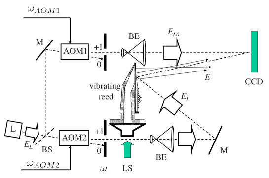
Figure 1: Holographic setup. L: main laser; AOM1, AOM2: acousto-optic modulators; M: mirror; BS: beam splitter; BE: beam expander; CCD: CCD camera; LS: loudspeaker exciting the clarinet reed through the bore of a clarinet mouthpiece at frequency $f=\omega/2\pi$.

The experimental setup is shown schematically in Fig. 1. A laser beam, with wavelength $\lambda=650$ nm (angular frequency $\omega_{L}$) is split into a local oscillator beam (optical field $E_{LO}$) and an illumination beam ($E_{I}$); their angular frequencies $\omega_{LO}$ and $\omega_{I}$ are tuned by using two acousto-optic modulators (Bragg cells with a selection of the first order diffraction beam) AOM1 and AOM2: $\omega_{LO}=\omega_{L}+\omega_{AOM1}$ and $\omega_{I}=\omega_{L}+\omega_{AOM2}$, where $\omega_{AOM1,2}\simeq 2\pi\times 80$ MHz. The first beam (LO) is directed via a beam expander onto a CCD camera, while the second beam (I) is expanded over the surface of the reed, which vibrates at frequency $f$ . The light reflected by the reed (field $E$) is directed toward the CCD camera in order to interfere with the LO beam ($E_{LO}$). 4 phases were used (phase shifting digital holography) and we select the first sideband of the vibrating reed reflected light by adjusting $\omega_{AOM1,2}$ to fulfil the condition: $\omega_{AOM1}-\omega_{AOM2}=2\pi(f+f_{CCD})/4$, where $f_{CCD}$ is the CCD camera frame frequency. The complex hologram signal $H$ provided by each pixel of the camera, which is proportional to the sideband frequency component of local complex field $E$, is obtained by 4-phases demodulation: $H=(I_{0}-I_{2})+j(I_{1}-I_{3})$ where $I_{0}\ldots I_{3}$ are 4 consecutive intensity images digitally recorded by the CCD camera, and $j^{2}=-1$. From the complex hologram $H$, images of the reed vibration are reconstructed by a standard Fourier holographic reconstruction calculation [23]. These holographic reconstructed images exhibit bright and dark interference fringes. Counting these fringes provides the amplitude of vibration of the object (in the direction of the beam), which depends on the wavelength $\lambda$ of the laser, and on the first Bessel function $J_{1}$, for instance $\pm 95$nm for the first, $\pm 770$nm for the $5^{th}$ and $\pm 1.6\mu m$ for the $10^{th}$ maximum (bright fringes) [24, 25].

This method has 3 main advantages:

(i) The time for data acquisition is very short, about 3 minutes for recording 184 holograms, including holographic reconstruction.

(ii) The signal to noise ratio is significantly better than with traditional technology, particularly through the elimination of signal at zero frequency.

(iii) The visualization of large-amplitude vibration (order of magnitude: 0.1 mm) is possible by using high harmonics orders (up to several hundred times the excitation frequency).

2.1.2 Reed excitation

The reed was excited by a tweeter loudspeaker screwed onto an aluminium plate, connected to a clarinet mouthpiece. The lay of this mouthpiece was modified to be strictly flat. A plastic wedge of uniform thickness has been inserted between the lay and the reed, longitudinally to the same height as the ligature (Vandoren Optimum), allowing free vibrations of the entire vamp (length: about 38 mm), see Fig. 1. This ensures precise boundary conditions, avoiding any dependence to deformations of the reed. The repeatability of the longitudinal placing of the wedge and of the reed was ensured by a Claripatch ring [26].

This setup requires some comments:

(i) The reed is excited exclusively through the bore of the mouthpiece.

(ii) The pressure field in the chamber of the mouthpiece was not measured. Like for a real instrument, the edges of the reed (protected by the walls of the chamber) are subject to a pressure field, which is probably lower than the pressure acting on the rest of the vamp.

(iii) The boundary conditions are very different from those of a real instrument (no curved lay, no contact with the lip). In addition, the reed was not moistened for the measurement.

(iv) The excitation device is almost closed. The acoustical resonances of the excitation device are unknown, but may quite easily be deduced by comparing different measurements, because they are always present at the same frequency.

2.2 Observation of resonance frequencies

2.2.1 Experimental protocol

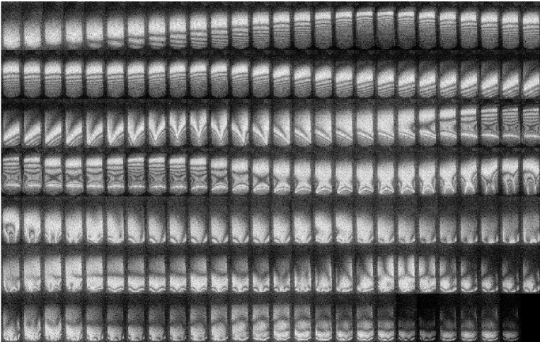
Figure 2: Typical holographic patterns of series A (asymmetrical sinusoidal excitation: the left side of the reed is more strongly excited than the right side). Frequency range: 1.4 to 20 kHz by steps of 25 cents (181 pictures ordered from left to right, continued on the next row; the tip of the reed is down on each picture). Some modes are easily identified: $F1$ (1st row, 19th picture), $T1$ (3rd row, 10th picture), $F2$ (4th row, 7th picture), $T2$ (4th row, penultimate picture), $X1$ (5th row, 5th picture) etc … Modes $T3$ and $F3$ are almost at the same frequency (6th row, 4th and 5th pictures, probably). The last picture of the 3rd row corresponds to an acoustic resonance of the excitation device. It is present on all holograms of both series at the same frequency (examine Fig.3). The excitation amplitude exponentially increases until the 73rd picture (3rd line, 21th picture), being hold constant beyond.

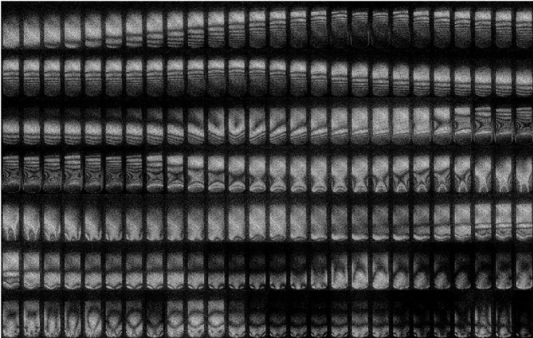
Figure 3: Typical holographic patterns of series B (symmetrical sinusoidal excitation). The modes $X1$ and $T3$ cannot be distinguished anymore. Notice that $T1$ is less marked than under asymmetrical excitation (for some reeds even difficult to identify) and that the pattern has a significant flexural component, strongly dependent of the lateral placing of the reed on the mouthpiece. Notice that the symmetry of the patterns near $T1$ depends on the excitation frequency.

55 clarinet reeds of model Vandoren V12 were purchased in a music shop: 12, 12, 20 and 11 reeds of nominal forces 3, $3\frac{1}{2}$, 4 and $4\frac{1}{2}$, respectively. 29 reeds were used for two preliminary studies in order to develop the measurement protocol. Each of these reeds was played a total of some tens of minutes, spread over several weeks before measurement with the final protocol. The other 26 reeds were strictly new by measurement, which was performed immediately after package opening (for 21 of them with the new hermetically sealed package by Vandoren, ensuring a relative humidity between 45 and $70\%$, according to the manufacturer), without moistening the reed.

Each reed was subject to 2 series of measurements:

• Series A (asymmetrical excitation: see Fig.2): the right half of the mouthpiece chamber was filled with modeling clay to ensure a good excitation of antisymmetrical modes. 184 holograms were made ranging from 1.4 to 20 kHz (sinusoidal signal), by steps of 25 cents. The amplitude of the excitation signal was exponentially increased in the range 1.4 to 4 kHz, from 0.5 to 16 V, then kept constant at 16 V up to 20 kHz. This crescendo limits the amplitude of vibration of the first two resonances of the reed. The temperature was not measured (about 20^∘C).

• Series B (symmetrical excitation: see Fig.3): the modeling clay was removed. The protocol is otherwise identical to this of the first series. The reeds were inadvertently exposed during one night to the very dry and warm air from the optical laboratory between the two series of measurements. The reeds lost between 2 and $4\%$ of their mass. In what follows we try to interpret the influence of this fact. The temperature was around 23-25^∘C.

2.2.2 Nomenclature of normal modes

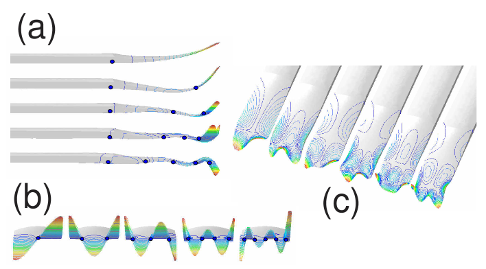
Figure 4: (a) Flexural modes $F1$, $F2$, $F3$, $F4$ and $F5$. Side view. (b) transversal modes $T1$, $T2$, $T3$, $T4$, $T5$. Front view. (c) Generic modes: $X1$, $X2$, $X3$, $X4$, $X5$ and $X6$. View from above. The intersections of nodal lines with the sides of the reed are symbolized by the blue dots.

Distinguishing 3 morphological classes, we classify the modes of a clarinet reed as follow : i) The “flexural” (or “bending”, or “longitudinal”) modes, listed below $F$, whose frequencies mainly depend on the longitudinal Young modulus ($E_{L}$) and polarized mainly in the $z$ axis, ii) the “transversal” (or “ torsional”, or “twisting” ) modes, listed below $T$, mainly dependent on the shear modulus in the longitudinal / tangential plane ($G_{LT}$), and iii) the “generic” (or “mixed”) modes, listed below $X$, sensitive to both moduli $E_{L}$ and $G_{LT}$ (see Fig.4). A subclass of flexural modes may be distinguished: the “lateral” modes (listed below $L$), polarized mainly in the $y$ axis (see Fig. 5). These modes were not observed in our study.

The modes have been numbered after the order of increasing frequencies from a preliminary modal analysis we performed. In our analysis, however, the identification of a mode is based upon morphological criteria. As a matter of fact, the mode number and the order of observed frequencies are not necessarily identical for all reeds.

Strictly speaking, the optical method only allows to observe the resonance frequencies of the reed and not the eigenfrequencies. Therefore the observed deformation patterns are a priori not identical to the eigenmodes of the reed. Nevertheless in practice no major differences have be found between the computed eigenmodes (see Section 4) and the observed or computed deformation for a forced asymmetrical excitation at the corresponding frequency. For this reason we use the terminology “mode” for the maximum amplitude of the response of the reed to a forced excitation. This is somewhat abusive, because the small shift between the resonance frequencies due to damping and the eigenfrequencies computed by FEM, without damping, is ignored. Besides damping, the acoustic load is also able to shift the resonance frequencies. We assume that this discrepancy is approximatively the same for all reed.

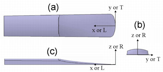
Figure 5: The clarinet reed: coordinates system. (a) top view, (b) front view, (c) side view. $x$, $y$, $z$: Cartesian axes of the object. L, T, R: axes of the orthotropic material (L: longitudinal, T: tangential, R: radial). In the software Catia used for the simulations, the orthotropic model is Cartesian and not cylindrical. Therefore an exact equivalence between $x,$ $y$, $z,$ and L, T, R respectively can be assumed since we observed no important deviation between the direction of the grain and the axe of symmetry of the reed.

2.2.3 Analysis of holograms; mode identification

More than 30000 holograms were made for this study and analyzed as follows: The picture where the number of interference fringes is locally maximum is determined. For some cases, we chose the hologram that is most similar to our numerical simulations (by Finite Element Method, see Section 4) or to other holograms (see Fig.6). The holograms corresponding to an acoustical resonance of the system, present at the same frequency (4309 Hz) for all reeds, have been eliminated. The identification of the different patterns to those calculated by FEM was often quite simple. An exception have been encountered for $F3$ and $T3$, whose frequencies were often so close that our identification is sometimes uncertain. More sophisticated techniques would certainly solve this problem. Notice that other boundary conditions (e.g. with clamping closer to the tip of the reed) would also easily separate these two modes. The frequency of some higher modes could not always be measured, either because their frequency was beyond 20 kHz, or because their pattern could not be clearly identified.

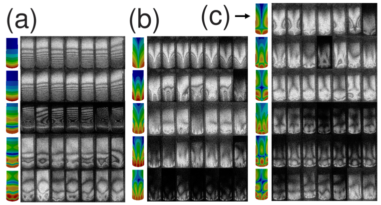
Figure 6: Qualitative comparison with FEM computation, and typical variability of the experimental results. (a) First row: Quasi-static pattern (at 605 Hz, with strong excitation by the LS). 2nd to 5th row: Flexural modes $F1$, $F2$, $F3$ and $F4$. Leftmost column: numerical simulation of eigenmodes by FEM. Columns 2 to 7: Arbitrary selection representing the observed variability (The first two rows correspond to the same selection of reeds). Notice the marked asymmetries and the differences in the curvature of the interference fringes near the tip of the reed. (b) Rows 1 to 5: transversal modes $T1$, $T2$, $T3$, $T4$ and $T5$ (probably). Columns: see (a). (c) Rows 1 to 6: Generic modes $X1$, $X2$, $X3$, $X4$, $X5$ and $X6$. The identification with $X6$ is sometimes unlikely. Columns: see (a).

3 Statistical analysis of resonance frequencies

4 flexural, 5 transversal, and 6 generic modes have been identified, namely all 15 first modes of the reed, excluding lateral modes. This number is significant, compared to the 4 modes detected by Pinard et al. [13]. The 6th mode ($L1$) could not be identified, as it is a lateral mode (flexural mode moving mainly in the $y$ axis), not excited by our loudspeaker. We tried to observe it by rotating the mouthpiece to the side, without success. Notice that higher modes could probably be identified using an ultrasonic loudspeaker.

3.1 Statistics

The statistics are displayed on Fig. 7 and detailed in Appendix A, with the analysis of correlations. For 14 measurements of resonance frequencies of the two series, identification of the total number of reeds (55) have been done. For other measurements, identification has been done only for a part of this number. The value of the ratio of the standard deviation $\sigma$ to the mean value $\mu$, i.e. the relative standard deviation, is found to be between 2 and 5% (about $1/3$ tone). If we admit Gaussian distribution for the measured frequencies, $99\%$ of the observations typically range about $\pm 1$ tone ($\pm 200$ cents) around the mean value (i.e. $\mu\pm 3\sigma$), for all frequencies.

The identification of the mode $X6$ is uncertain: it seems to appear for frequencies lower than those of our simulations. Mode $T5$ is on the limit of the range we studied: this explains the small value of the standard deviation.

Between series A and B, the flexural modes $F1$ to $F4$ lower their mid range, while the transversal modes slightly increase it. The difference between the two series probably lies mainly in the drying of the reeds, and this seems to have a statistically significant effect. This is surprising, because drying decreases the density of the reed, and theoretically this should proportionally increase all frequencies. In addition, according to Obataya et al. [11], drying is expected to increase $E_{L}^{\prime}$ (at least around 400 Hz), which should also increase the resonance frequencies. However Chevaux [7] observed that drying diminishes $E_{L}^{\prime}$ for material extracted from the inner side of the cane and augments slightly $E_{L}^{\prime}$ for material extracted nearer from the outer side (for cane suitable for oboe reeds), at least in the frequency range 100-500 Hz.

The hypothesis of an influence of the excitation method on the resonance frequencies seems unlikely, as well as the hypotheses of a poor reproducibility of the position of the reed on the mouthpiece between measurements or of the modification of the acoustic load, due to the modeling clay.

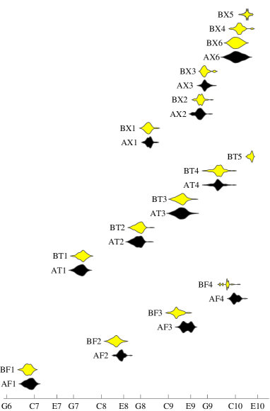
Figure 7: Observed resonance frequencies for the different reeds of each series, according to the results of Table 7. AF1 signifies mode F1, series A. The series A is in black, and the series B in white (yellow online). In abscissa the frequencies in logarithmic (musical) scale. From the left to the right, the different notes correspond to the following frequencies: 1568, 2093, 2637, 3136, 4186, 5274, 6272, 8372, 10548, 12544, 16744, 21096 Hz

3.2 Principal component analysis

Principal Component Analysis (PCA) is mathematically defined as an orthogonal linear transformation transforming the data to a new coordinate system, such that the greatest variance by any projection of the data comes to lie on the first coordinate (called the first principal component or first factor), the second greatest variance on the second coordinate, and so on [27]. Theoretically PCA is the optimum linear transform for given data in terms of least squares. PCA is based upon the calculation of the eigenvalue decomposition of the covariance (or of the correlation) matrix (see e.g. [22]).

A PCA has been performed using the FACTOR module of SYSTAT [28]. The 14 variables (observed frequencies) presenting complete measurements for all reeds have been selected (all variables having 55 identified pattern, $N_{A}$ or $N_{B}=55$, see Table 7). Frequencies are rated in cents.

The 4 largest eigenvalues have been selected. They capture $91.2\%$ of the total variance of our sample (respectively $53.6\%$, $21.4\%$, $10.8\%$ and $5.4\%$ for each factor). A fifth factor would capture only $2.5\%$ variance more. The 14-dimensional data have been linearly projected onto a 4-dimensional factor space.

The factor space can afterwards be orthogonally rotated, for instance for maximizing the correlations between rotated factors and observed variables. In the studied case, no a priori knowledge about the orientation of the factor space is available. For an easy comparison, using the VARIMAX algorithm, we choose to maximize the correlations between rotated factors and all available variables (observed resonance frequencies and theoretical components from the model described hereafter in Section 5.2).

	$factor_{1}$	$factor_{2}$	$factor_{3}$	$factor_{4}$
AT2	0.973	0.054	0.078	-0.008
BT2	0.953	0.055	-0.025	0.085
AT3	0.898	0.198	-0.237	-0.032
AX2	0.853	0.273	-0.073	-0.123
AT1	0.776	0.017	0.577	0.087
BT1	0.762	-0.033	0.541	0.177
AX3	0.761	0.472	0.090	0.217
AX1	0.740	0.451	0.356	0.115
AF3	0.223	0.891	0.076	0.080
AF2	0.143	0.791	0.519	0.064
AF1	0.085	0.360	0.870	-0.141
BF1	0.104	0.385	0.835	0.209
BF3	0.059	0.596	0.050	0.755
BF2	0.147	0.561	0.290	0.710
$e_{1}$	0.958	-0.080	0.105	0.005
$e_{2}$	0.059	0.969	0.082	0.098
$e_{3}$	-0.075	-0.073	0.971	0.042
$e_{4}$	-0.009	-0.081	-0.039	0.979

Table 1: Correlation (loadings) between rotated factors from PCA and : i) variables (measured resonance frequencies) or ii) components from viscoelastic model ($\boldsymbol{e}[n]$, see Section 5.2), for comparison, sorted in reverse order of magnitude. In bold:  greater correlation for each variable.

We performed also a PCA separately for each measurement series (A and B: 9 and 5 variables, respectively). From series A we detected 3 important factors capturing $90.8\%$ of the variance (56.9, 23.0, $11.0\%,$ respectively). From series B we detected also 3 important factors capturing $94.1\%$ of the variance (54.0, 26.8, $13.3\%$, respectively). A 4th factor would capture only $3.6\%$ more for series A and $3.4\%$ for series B. One factor seemingly disappeared, compared with the PCA performed on both series. A hypothesis is that this factor is related to the hygrometric change between the two series.

>From Table 1, we see that all transversal and generic modes are well correlated with $factor_{1}$; $factor_{2}$ correlates with high frequency flexural modes of both series (however notably better with those of series A); $factor_{3}$ well correlates with $F1$ of both series (and somewhat with other low frequency modes: AT1, BT1 and AF2), whereas $factor_{4}$ correlates quite well with high frequency flexural modes of series B.

3.3 Conclusions from the statistical analysis

Fifteen modes of vibration of the clarinet reed have been observed, while previous studies investigated 4 to 5 modes only [17, 13]. The observed resonance frequencies are often highly correlated, especially those among the “transversal” modes and, to a lesser extent, those among the “flexural”  modes. The nominal reed strength is surprisingly better correlated with the frequencies of “transversal” modes as with those of “flexural”  modes. The flexural modes within the same series are poorly correlated.

A principal component analysis of the resonance frequencies identifies 4 main factors, capturing $91.2\%$ of the variance of the sample. The data can therefore be reconstructed with 4 uncorrelated factors only (error: $RMSD=21.8$ cents, see Appendix D.2 and E). The effect of hygrometric change between both measurement series can seemingly be described with 1 factor only.

These statistical facts offer a guidance for modeling appropriately the mechanics of the clarinet reed.

4 Development of a mechanical model

4.1 Choice of a viscoelastic model

In the present study our concern is to develop a model with a minimal number of physically related components, that adequately reconstructs the observed resonance frequencies of our reeds. We presume that these components offer an objective characterization of the material composing each reed. A sensitivity analysis by FEM calculation assuming an orthotropic, elastic material has been conducted, and showed that the longitudinal Young modulus $E_{L}$ and the longitudinal / transverse shear modulus $G_{LT}$ play a leading role. Nevertheless taking into account the previous result of 4 factors given by PCA, we will see that an elastic model is not sufficient to establish a satisfactory model with 2 degrees of freedom only (i.e. variables $E_{L}$ and $G_{LT}$ per series. Therefore a viscoelastic model is sought.

It is well known that the stiffness of natural materials like wood or cane varies with the frequency of the applied stress and with the temperature. The material is stiffer at low temperature and at high frequency. At low frequency or high temperature the material is almost perfectly elastic and reaches the rubbery modulus. At high frequency or at low temperature the glassy modulus is reached; the material is almost perfectly elastic, also, but stiffer. At mid frequency or mid temperature, the apparent modulus (called storage modulus, i.e. the real part of the complex Young modulus for this frequency) is between the two values. For a particular frequency, called relaxation frequency, the storage modulus is exactly at the average of glassy and rubbery moduli. Around this frequency dissipation is maximum. Once the characteristic curve is known (for given temperature and different frequencies, or for given frequency and different temperatures), the Arrhenius equation offers usually an adequate estimate of the stiffness for any frequency and any temperature, within a quite broad range [29].

The determination of the mechanical parameters of a natural material requires to determine for each axis of the orthotropic material the value of 3 parameters (Young modulus, shear modulus and Poisson’s ratio). These 9 parameters may exhibit viscoelastic behavior, requiring theoretically for each one the fit of a viscoelastic model, such as the general linear solid (also called Zener model or 3-parameter model, see [29, 30, 31, 32]). The chosen model is based on 6 parameters (3 parameters for both variables $E_{L}$ and $G_{LT}$). Therefore the viscoelastic model (Section 4.4) has many degrees of freedom (6, for each of the 2 series of measurements, compared to the 4 factors detected by PCA for both series), for solving adequately the inverse problem (see Section 5 for the reduction of the number from 12 to 4).

4.2 Computation method

Considering viscoelasticity leads to complex modes with complex eigenfrequencies. Compared to the non-dissipative, elastic case computed by FEM, the main consequence of viscoelasticity, besides dissipation, is that stress and strain are not in phase. For sake of simplicity, we limit the computation to eigenfrequencies only, and assume that they depend on the storage moduli only (i.e. dissipation has a negligible influence). Having reduced the viscoelastic problem to an associated elastic one, the elastic solution may be used (see e.g. Ref. [29]). In order to compute the resonance frequency $\omega_{r}$ after an elastic model, according to Ref. [32], we admit that $E\simeq E^{\prime}(\omega_{r})$, where $E^{\prime}(\omega_{r})$ is the real part of the complex modulus in the frequency domain. This hypothesis implies that the calculation of the eigenfrequencies from the values of the storage modulus is done by an iteration procedure, and allows to use a FEM software (Catia) which does not allow computing with frequency-dependent coefficients.

Therefore we first present results of FEM simulations (Section 4.3), assuming an elastic and orthotropic behavior of the reed (modeled in Section 4.3.1). This helps to identify the modes in experiments, and allows obtaining a fit formula (Section 4.3.3) for computing the 11 lower resonance frequencies with respect to two parameters only, $E_{L}$ and $G_{LT}$, detected after a sensitivity analysis (Section 4.3.2). The fit formula, called "metamodel", is then used in the iterative procedure for the computation of the viscoelastic model. It allows a great reduction of computation time, compared to the FEM, and this is very useful for the inverse problem. Such a metamodel could be directly computed for the viscoelastic model with an appropriate software, but starting with the elastic model simplifies the fitting procedure.

4.3 Elastic model

4.3.1 Modeling the reed

The clarinet reed is defined in a Cartesian axis system $x,y,z$ (see Fig. 5). The origin is located in the bottom plane, at the tip of the reed. The material is defined as 3D orthotropic and assumed to be homogeneous, whose longitudinal direction L is parallel to the $x$ axis, the tangential direction T parallel to the $y$ axis and the radial direction R parallel to the $z$ axis.

The dimensions in the $xy$ plane are consistent with the measurements given by Facchinetti et al. [21]. The heel of the reed is made out of a cylinder section, diameter 34.8 mm, maximum thickness 3.3 mm. The shape of the reed is defined in Appendix B.

During playing, the reed has two contact surfaces with the ligature. For the present simulations, the reed is clamped in the same way than for normal playing, on two rectangular surfaces $23\times 1$ mm, spaced laterally by 5 mm, 38.2 mm from the tip of the reed, simulating the contact surfaces on the Vandoren Optimum ligature. However, unlike normal playing, the whole vamp of the reed is free to vibrate (see Figure 1).

For the simulations, the “Generative Part Structural Analysis” module by Catia v.5.17 (Dassault Technologies) is used, with mesh Octree3D, size 2 mm, absolute sag 0.1 mm, parabolic tetrahedrons. The generated mesh involves 5927 points, allowing both a good accuracy and a reasonable computing time (around 35 seconds).

4.3.2 Sensitivity analysis of elastic coefficients

Coefficient	$F$	$T$	$X$	$L$	All modes
$E_{L}$	0.4087	0.1053	0.1835	0.2093	0.2235
$G_{LT}$	0.0140	0.2681	0.1962	0.1067	0.1575
$E_{T}$	0.0076	0.0976	0.0741	0.0166	0.0562
$G_{LR}$	0.0438	0.0131	0.0257	0.0818	0.0341
$E_{R}$	0.0176	0.0120	0.0135	0.0662	0.0207
$G_{TR}$	0.0046	0.0092	0.0077	0.0215	0.0091
$\nu_{TR}$	0.0015	0.0009	0.0015	0.0054	0.0019
$\nu_{LT}$	0.0018	-0.0031	0.0004	0.0007	-0.0001
$\nu_{LR}$	0.0009	0.0002	0.0005	0.0013	0.0007

Table 2: One-At-a-Time sensitivity study by FEM: Averaged ratio between relative change in frequency and relative change for each elastic coefficient (i.e. $\pm 10\%$), sorted by decreasing order of magnitude, for the first 16 eigenmodes. $F$: flexural modes ($F1$ to $F4$), $T$: transversal modes ($T1$ to $T4$), $X$: generic modes ($X1$ to $X6$), $L$: lateral modes ($L1$ and $L2$; these modes were not observed in our study), All modes: averaged ratio over all modes. In bold: maximum absolute value for each coefficient of the orthotropic material: $E_{L}$, $E_{T}$ and $E_{R}$: Young moduli; $\nu_{LT}$, $\nu_{LR}$ and $\nu_{TR}$: Poisson coefficients; $G_{LT}$, $G_{LR}$ and $G_{TR}$: shear moduli.

For selecting the most relevant parameters, we conducted a One-At-a-Time sensitivity analysis [34], varying each coefficient by $\pm 10\%$ and computing the first 16 modes, based on the following reference values: $E_{L}=$14000 MPa, $E_{T}=E_{R}=$ 480 MPa, $\nu_{LT}$ $=\nu_{LR}=\nu_{TR}=$0.22, $G_{LT}=$ 1100 MPa, $G_{LR}=G_{TR}=$ 1200 MPa. The density $\rho$ was set to 520 kg/m³, according to the estimation by Guimezanes [17]. The results are shown in Table 2. Notice that $E_{L}$ and $G_{LT}$ plays a decisive role, while $E_{T}$ plays a marginal role and all other parameters have an almost negligible influence on the resonance frequencies. As a consequence, the moduli $E_{L}$ and $G_{LT}$ are the variables retained in the model. The approximate value of $E_{T}$ has been estimated according to the morphology of the patterns of higher order modes. This value is consistent with measurements given by Spatz et al. [1].

Notice that these results show the validity of a 2D approach, the reed being modeled as a thin plate. This should be used for further studies.

4.3.3 Metamodel approximating the resonance frequencies

The following analytic formula ("metamodel") predicts quickly and efficiently the resonance frequencies of a clamped/free clarinet reed. It was established in the following way: Frequencies of the first 16 modes were computed by FEM, according to a network of 92 separate pairs of values for $E_{L}$ and $G_{LT}$, ranging from 8000 to 17000 MPa and 800 to 1700 MPa, respectively. The other elastic coefficients were held constant, according to the reference values cited above. For the range of simulation values, this arbitrary formula (developed by trial and error) provides a very good fit (generally better than $\pm 5$ cents, see Table 9). Expected resonance frequencies $f$ are first found in $cents$ ($FC$) from the note F6 (1396.9 Hz), and finally in $Hz$:

$$f(m,E_{L},G_{LT}) = 1396.9\times 2^{FC/1200}\text{, where}$$ (1)

$$FC = a_{m,0}+a_{m,1}\,E_{p}+a_{m,2}G_{p}+a_{m,3}\,E_{p}\,G_{p}+a_{m,4}\,E_{p}^{2}+a_{m,5}G_{p}^{2}\text{,}$$

$$E_{p} = E_{L}~{}^{-0.66643}\text{ and\ }G_{p}=G_{LT}~{}^{0.7627}.$$

The index $m$ is the number of the mode defined in Appendix C, Table 9, where the values of the coefficients $a_{m,q}$ are given ($E_{L}$ and $G_{LT}$ are expressed in MPa).

The influence of the density is easy to predict: frequencies vary proportionally to $\rho^{-1/2}$. The computing cost of this metamodel is about $10^{7}$ times lower than with FEM, largely simplifying the inverse problem.

4.3.4 Efficiency of the metamodel

Equation (1) can be used to estimate the values of $E_{L}$ and $G_{LT}$, providing a faithful reconstruction of the observed resonance frequencies. Theoretically these values could be computed for any pair of modes, after their respective observed frequencies. Unfortunately, this method gives no consistent results. A least squares fit is a more robust technique for such a computation. This leads however to systematic errors in the predicted frequencies: low-order modes are systematically overestimated, while high-order modes are underestimated. This can be corrected by adjusting the coefficients $a_{m,0}$ (from Table 9), but this cannot explain the bad correlation among flexural modes within the same series (see Table 6). According to the elastic model, these correlations should be in all cases greater than 0.998. A hypothesis for resolving this contradiction is that the moduli are varying with the frequency in an individual way for each reed. Thus in the next paragraph we consider a viscoelastic model, where $E_{L}$ and $G_{LT}$ are frequency dependent. This leads to the addition of some parameters, which are to our mind more important that the other elastic coefficients. The fit of such a model requires many observations at different frequencies, in order to reduce the influence of measurements errors and of local irregularities in the structure of cane.

Alternative hypotheses could be considered in this context, as damping, acoustic load [21], local variations in stiffness or in density, local deviations in thickness, compared to the assumed theoretical model. However, these hypotheses are probably unable to explain the hygrometric-induced individual variations we observed for each reed, thus our preference for the viscoelastic hypothesis.

4.4 Viscoelastic model

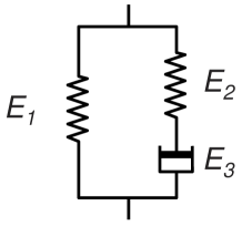
Figure 8: Schematic representation of the standard linear solid: two springs $E_{1}$, $E_{2}$ and a dashpot $E_{3}$.

In this section, a Zener model is considered (see e.g. Refs [29, 30, 31, 32]). This model is applied to both moduli $E_{L}$ and $G_{LT}.$ The scheme of the standard viscoelastic solid is presented on Fig.8, with two springs $E_{1}$ and $E_{2}$ and a dashpot $E_{3}$. At low frequencies, $E_{2}$ and $E_{3}$ have practically no effect (the rubbery modulus $E_{1}$ dominates). At high frequencies, $E_{3}$ has practically no effect (the glassy modulus $E_{1}+E_{2}$ dominates). In the frequency range near $E_{2}/(2\pi E_{3})$ the dissipation due to $E_{3}$ is maximal and the apparent modulus (storage modulus) is in the mid-range. The stress $\sigma$ and the strain $\varepsilon$ are related by the constitutive equation:

$$\sigma+\tau_{1}\dot{\sigma}=E_{1}(\varepsilon+\tau_{2}\dot{\varepsilon})$$ (2)

in which $\tau_{1}={E}_{3}/{E_{2}}$ is called the relaxation time and $\tau_{2}={E}_{3}{(E_{1}+E_{2})}/{(E_{1}E_{2})}$ the retardation time. $E_{1}$ is called rubbery modulus and $E_{1}+E_{2}$ glassy modulus. In harmonic regime, for an angular frequency $\omega$, the Young modulus is complex:

$$E^{\ast}(\omega)=E_{1}+E_{2}-\frac{E_{2}^{2}}{E_{2}+j\omega E_{3}}=E_{1}+E_{2}+\frac{-E_{2}+j\omega E_{3}}{1+\left(\omega E_{3}/E_{2}\right)^{2}}$$ (3)

The second formulation separates the real part ($E^{\prime}(\omega)$: storage modulus) and the imaginary part ($E^{\prime\prime}(\omega)$: loss modulus) of $E^{\ast}(\omega)$. The storage modulus can thus be written as:

$$E^{\prime}(\omega)=E_{1}+E_{2}-\frac{E_{2}^{3}}{E_{2}^{2}+\omega^{2}E_{3}^{2}}=E_{1}\frac{1+\omega^{2}\tau_{1}\tau_{2}}{1+\omega^{2}\tau_{1}^{2}}.$$ (4)

Notice the properties:

$$E^{\prime}(0)=E_{1}\text{ ; \ }E^{\prime}({1}/{\tau_{1}})=E_{1}+E_{2}/2$$

$$E^{\prime}(\infty)=E_{1}+E_{2}\text{ ; }\frac{\partial E^{\prime}}{\partial\omega}\Big{(}\frac{1}{\tau_{1}}\Big{)}=\frac{E_{3}}{2}.$$

For the sake of simplicity, the parameters corresponding to $E_{L}$ and $G_{LT}$ are denoted $E_{1},$ $E_{2}$, $E_{3}$, and $G_{1}$, $G_{2}$, $G_{3}$, and the storage moduli given by Equation (4) $E^{\prime}(\omega)$ and $G^{\prime}(\omega)$, respectively. Therefore for each reed (and each series), the model requires 6 parameters instead of 2 (while experiments gave 4 main factors only for the whole set of results).

>From the knowledge of the 6 parameters, the resonance frequencies can be deduced by an iteration procedure. For each mode the starting point of the iteration is the mean value $f^{(0)\text{ }}$of the experimental resonance frequency (see Table 7), then the storage moduli are deduced from Equation (4), then a new value $f^{(1)}$ by using Equation (1), etc… The convergence of the iteration method is fast, actually one iteration is enough. This can be understood by the fact that the derivative of the iterated function is small (notice that the two first rows of Table 2 correspond to the derivative of $E_{L}$ and $G_{LT}$ with respect to frequency). If we give an arbitrary value, for instance $f^{(0)}=6000$, one iteration more is required for a comparable precision. In all hypotheses (see Appendix D.6), we used one iteration only. This procedure allows the determination of $f(m)$ from the coefficients $E_{1},$ $E_{2}$, $E_{3}$, $G_{1}$, $G_{2}$, $G_{3}$ for a given reed and a given series.

5 Inverse problem and selection of a robust model

5.1 Simplification of the model by multiple regression

In order to solve the inverse problem for each reed (and each series), we use a classical Mean Squared Deviation method, from the experimental values of the 11 resonance frequencies listed in Table 9 (see Appendix C). The results are given and discussed in Section 5.3.

However for each reed the viscoelastic model provides 12 parameters, i.e., 12 DoF, and the PCA showed that this number needs to be reduced. Actually this model conducts sometimes to non-physical results (negative rubbery modulus, for instance). This problem comes out because the observed resonance frequencies are far from 0, so the rubbery modulus $E_{1}$ cannot be estimated precisely. For that purpose multiple regression (see Appendix D for details) is used, by introducing correlations among parameters and reducing the degrees of freedom to a number of 4, called “components", which are linearly related to the parameters. The 4 components are very similar to the 4 factors computed by the PCA, but, because Eqs. (1 and 4) are nonlinear, a small deviation is inevitable for optimal results. Factors and components are consequently strongly correlated (>0.95, see Table 1).

We tested different hypotheses to establish a satisfactory robust model (denoted H1 to H9 and described in Appendix D), together with the detailed computation method. Each hypothesis leads to a given number of components related to the parameters through the regression coefficients. Notice that the parameters and components depend on both the reed and series, while the regression coefficients which correlate the parameters are independent of the reed and the series. A constant value elastic model (the parameters are fixed, and do not depend on the reed or the series, Hypothesis H1) is not sufficient. Similarly a 2-parameter elastic model ($E_{L}$ and $G_{LT}$, independent of the series, Hypothesis H2) is not sufficient as well. Conversely a linear model without constraints (with 60 independent coefficients, corresponding to a matrix of order 12(4+1) elements, Hypothesis H7) is not necessary, because many coefficients are very small. Eventually a 9 coefficient linear model (H4) has been found to be very satisfactory and is described in Section 5.2. The following ideas were applied: after eliminating the very small coefficients and fitting the observations with the remaining coefficients, it is observed that the predictive quality of the model is almost not affected by the simplification. This was done step by step. The problem of non-physical values for certain parameters can be corrected by setting that the damping parameters $E_{3}$ and $G_{3}$ are constant, independent of the reeds and of the series (typical values: $E_{3}=$ 0.28 and $G_{3}=$ 0.02). It remains 4 parameters for each series and reed, $E_{1}$, $E_{2}$ and $G_{1}$, $G_{2}$ (i.e. 8 parameters for each reed). This ensures generally that these parameters fall in a plausible range, when fitting the model. Moreover a hierarchical structure can be introduced in the model, isolating the hygrometric component, bringing the remaining 3 components to a common basis (Section 5.2) and simplifying the problem (reduced to only 9 regression coefficients) and giving some insight in the data structure.

The $RMSD$ (Root Mean Square Deviation, see Appendix D.2) is found to be 30.4 cents for Hypothesis H4, very close to 29.8 cents for H5 with 9 coefficients more. Moreover the standard deviation of the residuals for Hypothesis H4 (and also Hypothesis H5) varies very few over the different resonance frequencies (all around 30 cents).

The fit quality cannot be considered as a perfect and definitive proof that our model reflects the true values of the corresponding storage moduli. The influence of some missing parameters in the model should be examined (for instance differences in thickness between reeds, non constant modulus $E_{T}$, non constant density $\rho$ or radial variation of $E_{L}$). Anyways, the presented model reflects real mechanical differences between the reeds, very similar to those objectively detected by the PCA.

5.2 Robust estimation of the parameters of the viscoelastic model (Hypothesis H4)

Hypothesis H4 is chosen so that no coefficient can be removed without impacting notably the quality of fit. It can be thought as the minimal structure allowing an adequate reconstruction of the observed resonance frequencies, in conjunction with the viscoelastic model (Eq. (4)) and the metamodel (Eq. (1)). This minimal structure makes the model more robust against measurements errors, even if it probably introduces some bias.

As a first step, our concern is to eliminate the influence of the moisture content and to bring both series of measurements to a common basis (i.e. predict the effect of drying on the viscoelastic parameters of series B, the series A being taken as a reference). $e_{1}[n]$, $e_{2}[n]$, $e_{3}[n]$ and $e_{4}[n]$ are the 4 independent components characterizing the mechanical properties of the reed $n$. The choice of the notations is as follows: $e_{k}[n]$ is the $k$th element of the vector $\mathbf{e}[n].$, which depends on $n$. These components are conditioned similarly to PCA as orthogonal factors: mean 0, standard deviation 1 and intercorrelation 0. The elimination of the moisture content can be achieved by reducing the components to a number of 3 for each series $s=1$ (series A) and $s=2$ (series B): for reasons explained in Appendix D.4, these components are denoted $\check{e}_{1}[s,n]$, $\check{e}_{2}[s,n]$ and $\check{e}_{3}[s,n]$ .

For series A, the components remain unmodified (series A is taken as reference):

$$\check{e}_{1}[s=1,n]=e_{1}[n]$$

$$\check{e}_{2}[s=1,n]=e_{2}[n]$$

$$\check{e}_{3}[s=1,n]=e_{3}[n]$$ (5)

For series B, the effect of drying on the components is predicted by:

$$\check{e}_{1}[s=2,n]=c_{10}+e_{1}[n]$$

$$\check{e}_{2}[s=2,n]=c_{20}+\frac{1}{2}(e_{2}[n]+e_{4}[n])$$

$$\check{e}_{3}[s=2,n]=c_{30}+e_{3}[n]$$ (6)

With this choice of components, the viscoelastic parameters of the model for series $s$ and reed $n$ can then be estimated as follows:

$$E_{1}=d_{10}+d_{12}(\check{e}_{2}[s,n]+\check{e}_{3}[s,n])$$

$$E_{2}=d_{20}+d_{12}(2\check{e}_{2}[s,n]-\check{e}_{3}[s,n])$$

$$E_{3}=d_{30}$$

$$G_{1}=d_{41}(6+\check{e}_{1}[s,n])$$

$$G_{2}=2d_{41}(3+\check{e}_{1}[s,n]-\check{e}_{3}[s,n])$$

$$G_{3}=d_{60}$$ (7)

This implies some other interesting relationships:

$$E_{1}+E_{2}=d_{10}+d_{20}+3d_{12}\check{e}_{2}[s,n]$$

$$G_{1}+G_{2}=d_{41}(12+3\check{e}_{1}[s,n]-2\check{e}_{3}[s,n])$$

$$2E_{1}-E_{2}=2d_{10}-d_{20}+3d_{12}\check{e}_{3}[s,n]$$

$$2G_{1}-G_{2}=2d_{41}(3-\check{e}_{3}[s,n])$$ (8)

Notice that the glassy modulus of $E_{L}$ (i.e., $E_{1}+E_{2}$) depends linearly only on $\check{e}_{2}[s,n]$. The quantities $2E_{1}-E_{2}$ and $2G_{1}-G_{2}$ depend linearly only on $\check{e}_{3}[s,n]$, however with opposed signs.

The values of the 9 coefficients are: $c_{10}$=1.011, $c_{20}$= -2.197, $c_{30}$=0.8294, $d_{10}$=10300, $d_{12}$=640.5, $d_{20}$=7309, $d_{30}$=0.2822, $d_{41}$=115.7, $d_{60}$=0.02038. The coefficients in Eq. (1) are adjusted (in order to remove systematic errors) by adding to $a_{m,0}$ (from Table 9) the following values, for $m=1$ to 11: -26.27, 32.24, -50.05, 4.80, -26.87, -65.28, -48.64, 0.07, -52.98, -76.61 and -111.55 cents.

The change in density between the two series of measurements was not measured precisely (about -2 to $-4\%$). In the model, density is considered as constant.

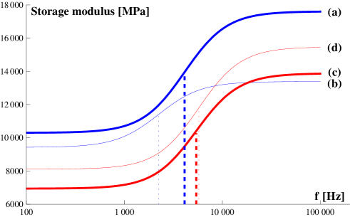
Figure 9: Hypothesis H4: plot of the storage moduli $E_{L}^{\prime}(\omega)$ and $G_{LT}^{\prime}(\omega)$ [in MPa], according to Equations (4 to 7), computed for the mean value of all reeds. (a): $E_{L}^{\prime}$ series A, (b): $E_{L}^{\prime}$ series B, (c): $G_{LT}^{\prime}$ series A and (d): $G_{LT}^{\prime}$ series B. For $G_{LT}^{\prime}$, the moduli are multiplied by 10. The abscissa of the relaxation frequencies [in Hz] is denoted by dashed lines (series A) and dotted lines (series B). The corresponding numerical values are listed in Tables 4 and 5. Only the portions of the curves between 2 and 18 $kHz$ could be fitted adequately. The curves outside this range are purely hypothetical: we have no measurements.

Fig. 9 shows an approximation of the frequency dependence of $E_{L}$ and $G_{LT}$, computed for the mean value of all reeds. For Series A, the storage modulus $E^{\prime}(\omega)$ increases from $11700$ MPa at 2 kHz ($F1$) to $17200$ MPa at 16.8 kHz ($F4$), while for Series B, it increases from $11100$ to $13300$ MPa. Therefore under "normal" hygrometry the reed bends in a notably viscoelastic manner, whereas the ultra-dry reed bends in an more elastic manner. For $G_{LT}$, the reed is generally notably viscoelastic, according to our model. The corresponding values are: 783 to 1290 MPa for Series A, and 896 to 1436 MPa for Series B. Corresponding statistics are displayed on Table 3. Drying seems to increase $G_{LT}$ and decrease $E_{L}$ (except around 2300 Hz), explaining the good correlation between the variables AF1 and BF1.

Increase in	$E_{L}$		$G_{LT}$
storage modulus	Series A	Series B	Series A	Series B
Mean	$~{}~{}31\%$	$~{}~{}16\%$	$~{}~{}38\%$	$~{}~{}36\%$
Standard deviation	$~{}~{}~{}5\%$	$~{}~{}~{}6\%$	$~{}~{}10\%$	$~{}~{}~{}9\%$
Minimum	$~{}~{}20\%$	$~{}~{}~{}1\%$	$~{}~{}13\%$	$~{}~{}15\%$
Maximum	$~{}~{}44\%$	$~{}~{}32\%$	$~{}~{}52\%$	$~{}~{}49\%$

Table 3: Optimal 9-coefficients model (hypothesis H4): Statistics of the frequency-dependent increase in storage modulus (for Series A or B and $E_{L}$ or $G_{LT}$), between the $1^{st}$ and the $4^{th}$ flexural mode: $1-E^{\prime}(2\pi f_{F1})/E^{\prime}(2\pi f_{F4})$ or $1-G^{\prime}(2\pi f_{F1})/G^{\prime}(2\pi f_{F4})$, with $f_{F1}=1996$Hz and $f_{F4}=16784$Hz. Between both series, the correlation is 0.83 for $E_{L}$ and 1 for $G_{LT}$ (as a consequence of the simplification of the model)

.

This simplified model permits interesting conclusions about the structure of our data:

• The component $e_{1}$ is related exclusively to $G_{LT}$;

• $e_{2}$ is related exclusively to $E_{L}$;

• $e_{3}$ increases proportionally to the rubbery modulus of $E_{L}$ (and not its glassy modulus), and decreases proportionally to the glassy modulus of $G_{LT}$ (and not its rubbery modulus); it regulates therefore the viscous component common to $E_{L}$ and $G_{LT}$;

• $e_{4}$ takes into account the variation in moisture content between series A and B.

Notice that the product of the rubbery moduli for the series A, $E_{1}G_{1}$ is correlated at $72\%$ with the nominal reed strength. Individually, these moduli correlate only at $50\%$ and $55\%$ with the nominal reed strength, respectively.

5.3 Results and discussion

Tables 4 and 5 show our results for hypotheses H4 and H5. A comparison with results by other authors is difficult or even quite impossible, because of the disparate structure of the measurements. Such a comparison requires the reconstruction of the measurement data (when possible), the fit of a viscoelastic model or the extrapolation of the values, in order to reach the frequency and temperature range of our measurements. The validity of such a highly speculative task is questionable. For the storage modulus $E_{L}^{\prime}$, all reconstructed values from other authors fall in the range around the average of our measurements $\pm 3$ times the standard deviation, however most of the time in the lower range. This probably shows that the selected value for the density $\rho$ is somewhat too high. No representative statistics are available by the other authors.

Model	Storage Young modulus $E^{\prime}_{L}(\omega)$ at about $20^{\circ}C$
	$E_{1}$ [MPa]	$E_{2}$ [MPa]	$f_{r}$ [Hz]	$E^{\prime}_{L}$ at 4 kHz
Hypothesis H4, series A	10300, SD 906	7309, SD 1432	4123, SD 808	13781, SD  897
Hypothesis H5, series A	9377, SD 844	8336, SD 1552	4027, SD 750	13449, SD  839
Hypothesis H4, series B	9423, SD 784	3964, SD 1109	2236, SD 626	12338, SD  885
Hypothesis H5, series B	7844, SD 753	5459, SD 1217	1947, SD 434	12168, SD  882

Table 4: Summary of our results for hypotheses H4 and H5 about the viscoelastic behavior of the longitudinal Young modulus $E_{L}$ in cane. $E_{1}$, $E_{2}$ and $f_{r}$ (relaxation frequency): parameters from Zener model. $E^{\prime}_{L}$ at 4 kHz : storage modulus at 4 kHz [in MPa]. SD: standard deviation (the value preceding SD is the average). The model is valid only between 2 and 18 kHz.

Model	Storage Shear modulus $G^{\prime}_{LT}(\omega)$ at about $20^{\circ}C$
	$G_{1}$ [MPa]	$G_{2}$ [MPa]	$f_{r}$ [Hz]	$G^{\prime}_{LT}$ at 4 kHz
Hypothesis H4, series A	694, SD 116	694, SD 327	5420, SD 2555	926, SD 102
Hypothesis H5, series A	752, SD 119	628, SD 328	6310, SD 3296	924, SD 105
Hypothesis H4, series B	811, SD 116	736, SD 327	5749, SD 2555	1042, SD 99
Hypothesis H5, series B	774, SD 119	769, SD 328	5622, SD  2401	1022, SD 103

Table 5: Summary of our results for hypotheses H4 and H5 about the viscoelastic behavior of the shear modulus in longitudinal / tangential plane $G_{LT}$ in cane. $G^{\prime}_{LT}$ at 4 kHz: storage modulus at 4 kHz. Same structure as Table 4. The model is valid only between 2 and 18 kHz.

The most important disagreement, compared with our model (hypotheses H4 and H5), is about the relaxation frequency. The explanation is probably because the studied frequency range was not same. For $G_{LT}$, we found no viscoelastic measurements by other authors. Our results are summarized in Tables 4 and 5. For $E^{\prime}_{L}$, between hypotheses H4 and H5, $f_{r}$ and $E^{\prime}_{L}$ at 4 kHz agree well, whereas $E_{1}$ and $E_{2}$ diverge by about 1-2 SD. This divergence comes because the observed frequency range was not broad enough. For the shear modulus, $G_{1}$ and $G_{2}$ are in good agreement for both hypotheses (and consequently $f_{r}$ and $G^{\prime}_{L}$ at 4 kHz also).

Our model is valid only for "ambient dry" reeds (since the ultra-dry conditioning was not controlled), in a frequency range which should not exceed one decade. We checked that a fractional derivative model after Gaul et al. [32] is not necessary in our narrow frequency range. Such models are however really efficient to cover a broad frequency range. For instance, the data by Lord for dry material [12] could be fitted very well ($E_{0}=8108$ MPa, $E_{1}=2964$ MPa, $p=0.298$ MPa$\cdot$s^α, $\alpha=0.546$). Notice that the order of the derivative ($\alpha$) is 1 in our viscoelastic model.

Our viscoelastic model is able to partially explain the bad correlations observed between flexural modes. In Table 6, the correlations are compared among observed resonance frequencies and computed modal frequencies, according to the viscoelastic model (hypothesis H4 and H5). It seems that additional hypotheses (such as an irregular thickness) should perhaps be considered for improving the model. However, we should remember that the determination of resonance frequencies are attached with some uncertainties, especially for the modes $F3$ and $T3$.

In order to clarify this issue, let us examine if the residuals (observed resonance frequencies minus computed modal frequencies with hypothesis H5) contain some pertinent information. A PCA shows that perhaps 2 residual factors contain some interesting information (explaining $30\%$ and $18\%$ of the residual variance). The first residual factor is correlated with AT3 (0.86), BT2 (0.74), AT2 (0.73) and AX2 (0.66). All these modes depend strongly on $G_{LT}$. An adjustment of the coefficient $a_{m,2}$ from the metamodel for the transverse modes could probably cancel this systematic bias (remember that the coefficients $a_{m,q}$ are computed from a theoretical model, which is probably also biased). Indeed, an increase by 14, 21, 16 and $11\%$ of this coefficient affecting the modes $T1$, $T2$, $T3$ and $T4$ makes the $RMSD$ drop from 29.8 to 28.5 cents. The second residual factor is correlated with AF1 (0.36), AF2 (0.29), AT2 ($-0.29$), BF1 (0.28) and BT1 ($-0.23$). This probably reveals a competition between flexural and transversal modes when fitting the model. The bias probably comes from the coefficient $a_{m,1}$, regulating the linear dependance to $E_{L}$ in the metamodel. Adjusting the coefficients $a_{m,1}$ for all modes and the coefficients $a_{m,2}$ for all transverse and generic modes makes the $RMSD$ drop down to 26.2 cents, reaching the size of the measurement steps (25 cents). The adjustments of $a_{m,1}$ are very small for the flexural modes $F1$ to $F4$: -6, 1, 6 and $1\%$.

This shows that the most important bias depends linearly on the 2 most important parameters ($E_{L}$ and $G_{LT}$) of our FEM computations. No supplementary parameter is required until this bias is removed (theoretically down to a $RMSD$ of 21.8 cents, according to H10). For hypothesis H4, the same linear adjustment of the metamodel lets the $RMSD$ drop from 30.4 down to 27.0 cents.

Model	Mode	$AF1$	$AF2$	$AF3$	Mode	$BF1$	$BF2$	$BF3$
	$AF2$	0.73			$BF2$	0.63
observations	$AF3$	0.34	0.75		$BF3$	0.43	0.84
	$AF4$	0.28	0.65	0.74	$BF4$	0.00	0.43	0.45
	$AF2$	0.93			$BF2$	0.79
H4	$AF3$	0.69	0.90		$BF3$	0.62	0.97
	$AF4$	0.56	0.81	0.98	$BF4$	0.36	0.82	0.91
	$AF2$	0.90			$BF2$	0.69
H5	$AF3$	0.57	0.87		$BF3$	0.52	0.98
	$AF4$	0.43	0.77	0.98	$BF4$	0.26	0.84	0.92

Table 6: Correlations of resonance frequencies between flexural modes within the same series, after observations and viscoelastic models H4 and H5. $AF1$, $AF2$, $AF3$, $BF1$, $BF2$ and $BF3$: correlations with modal frequencies $F1$, $F2$ and $F3$ within series A or series B. Lines: corresponding flexural mode between which the correlations are computed.

6 Conclusion

The numerical model is satisfactory. From the statistical analysis are discussed in Section 3.3, it allows selecting the most important parameters describing the mechanical behavior of a reed.

The efficient elastic metamodel can be extended to a viscoelastic behavior of the reeds, approximating the resonance frequencies from the longitudinal Young modulus $E_{L}$ and the longitudinal / transverse shear modulus $G_{LT}$ and considering the hypothesis of their frequency dependence. A reconstruction of the observed resonance frequencies can be achieved with a good accuracy, estimating for each reed only 4 components, from which the parameters of a viscoelastic model are computed as a linear combination. The selected model (according to hypothesis H4) is probably slightly biased, but it is more robust against measurement errors than more refined models.

Table 1 shows that these components are highly correlated to the factors computed by PCA (0.96 to 0.98).

The proposed method allows the determination of 3 mechanical parameters characterizing the material composing each reed, with a single series of measurements, using Equations (1, 4 and 7). The reed should be conditioned with a relative humidity corresponding to the one ensured by the hermetically sealed package by Vandoren (about $55\%$). The fourth parameter cannot be determined in a reproducible way, since the exposure of the reeds to the ultra-dry air of the optical laboratory was not controlled. The same protocol and the same viscoelastic model can be used for other kinds of single reeds (bass clarinet, saxophone). Only the coefficients of Table 9 have to be recomputed after a FEM simulation of the corresponding reed shape.

Despite the fact that the eigenmodes of higher order probably play no important role in the acoustics of the clarinet, the present study shows that they reveal the inner structure of the material building the tip of the reed, so a new step could be done for an objective mechanical characterization of the clarinet reed. A subsequent study should examine if the obtained components are correlated with some musical qualities of the reeds. This could help the reed makers to gain a better control on their products.

Acknowledgments

We express gratitude for the financial aid from association DEPHY of the "département de physique de l’ENS", and to Fadwa Joud for her help during the experiments. The Haute-Ecole ARC (Neuchâtel, Berne, Jura) provided the software for simulation and calculation, and offered helpful instructions. The Conservatoire neuchâtelois partially supported this study for nearly 3 years. We also thank Bruno Gazengel, Morvan Ouisse and Emmanuel Foltête for fruitful discussions, and the referees for useful suggestions.

APPENDICES

Appendix A Statistics and correlations

The table 7 gives the detailed statistics.

	Series A					Series B
Mode	$N_{A}$	$\mu$	$\sigma$	$\mathbf{\min}$	$\mathbf{\max}$	$N_{B}$	$\mu$	$\sigma$	$\mathbf{\min}$	$\mathbf{\max}$
F1	55	1996	77	1838	2154	55	1960	66	1812	2093
T1	55	3377	132	3091	3676	55	3436	129	3136	3729
F2	55	5130	161	4767	5669	55	4856	189	4435	5351
T2	55	6108	261	5587	6939	55	6193	247	5669	7040
X1	55	6869	198	6455	7458	45	6801	217	6363	7458
T3	55	9571	500	8617	11014	54	9590	458	8742	11014
F3	55	10146	419	9262	10857	55	9213	414	8372	10396
X2	55	11521	387	10701	12187	54	11688	379	10857	13098
X3	55	12294	368	11502	13482	11	12290	471	11839	13482
T4	53	14011	756	12186	16503	54	14111	763	12186	16503
F4	45	16784	552	15803	18524	54	15363	663	14079	17484
X6	41	16984	972	15133	18793	30	16888	734	15577	18258
X4	24	18497	518	17234	19067	23	17544	772	16033	19911
X5	0					54	18896	501	17484	19911
T5	0					14	19668	329	19067	19911
Total	658					668

Table 7: Observed resonance frequencies, sorted by frequency (in Hz). $N_{A}$ (resp. $N_{B}$): Number of identified pattern for each mode of series A (resp. B). $\mu$: Mean value of the resonance frequency, $\sigma$: Standard deviation, $\mathbf{\min}$: Minimum, $\mathbf{\max}$: Maximum. Total: total number of identified patterns for each series.

Linear correlations have been computed between all possible couples of variables in a usual way (all the variables from Table 7, except $X5$ and $T5$ of series A, i.e. 13 variables for series A and 15 for series B, plus the nominal reed strength). Results of series A for the mode $F1$ are denoted AF1, and similarly for the other results. The following 12 pairs have a correlation greater than 0.9: AF1/BF1, AT1/BT1, AT2/BT2, AT3/AT4, AT3/BT3, AT3/BT4, BT3/BT4, AT4/BT3, BX1/BX3, AT4/BT4, BT4/BX6 and BX3/BX4. 54 pairs of variables have a correlation between 0.8 and 0.9, 50 other pairs between 0.7 and 0.8 and 262 other pairs, below 0.7.

Between the two series, the correlation is excellent for corresponding transversal modes ($T1$ (i.e. AT1/BT1): 0.97, $T2$: 0.97, $T3$: 0.96 and $T4$: 0.98), and generally good for corresponding generic modes ($X1$: 0.87, $X2$: 0.84, $X3$: 0.87 and $X4$: 0.55). For flexural modes, the correlation is good for $F1$ and progressively lower for increasing mode order ($F1$: 0.92, $F2$: 0.66, $F3$: 0.57 and $F4$: 0.47).

Within the same series, on the contrary, there is a poor correlation between AF1 and all measurements of series A, and similarly for BF1 and series B. This is striking: the two best correlated variables are AF2 and AX1 (0.73 and 0.49, respectively) for AF1 and BF2 and BT1 (0.63 and 0.49, respectively) for BF1. Moreover, these correlations are quite low among all flexural modes: see Table 6. This fact is discussed in section 5.3.

The nominal reed strength correlates at 0.7 with AT1 and AX4. We expected a better correlation with $F1$ (only 0.6). This is surprising, since the reeds were probably sorted by a quasi-static bending method by the manufacturer. This would mean that the storage modulus of $E_{L}$ at very low frequency is not well correlated with its value at the frequencies of the measured resonances. The influence of density has also to be considered. However, Obataya et al. [9] observed a good correlation between density and $E_{L}$. This point has to be investigated (see also section D.4 in Appendix D).

Appendix B Defining the shape of the reed

x [mm]	$s_{0}$ [mm] y=0 mm	$s_{1}$ [mm] y=4mm	$s_{2}$ [mm] y=6mm
0	0.074	0.080	0.042
5	0.343	0.293	0.197
10	0.648	0.542	0.377
15	1.047	0.847	0.571
20	1.451	1.135	0.745
25	1.926	1.527	1.078
30	2.540	2.084	1.589
35	3.351	2.817	2.256

Table 8: Network of points for interpolating the thickness of the vamp. See explanations in the text.

The thickness of the vamp at point $(x,y)$ is interpolated as follows: first, we interpolate 3 points at $y$=0, 4 and 6mm, with 3 cubic splines, according to Table 8. These three points ($s_{0}(x)$, $s_{1}(x)$ and $s_{2}(x)$) define a biquadratic polynomial:

$$vamp(x,y)=p_{0}(x)+p_{1}(x)\,y^{2}+p_{2}(x)\,y^{4}$$

with $p_{0}(x)=s_{0}(x)$, $p_{1}(x)=(-65\,s_{0}(x)+81\,s_{1}(x)-16\,s_{2}(x))/720$ and $p_{2}(x)=(5\,s_{0}(x)-9\,s_{1}(x)+4\,s_{2}(x))/2880$, allowing an interpolation on the $y$ axis. The network of points above was estimated using a least squares fit, based on a network of $12\times 24$ thickness measurements, achieved with a dial indicator and a coordinates-measuring table (estimated accuracy: $\pm 5\mu m$ in $z$, $\pm 50\mu m$ in $x$ and $y$). We measured twenty reeds and select a particularly symmetrical one as reference. This method allows the reconstruction of the measurement network with an accuracy of $\pm 10\mu m$.

The thickness of the heel is defined to be :

$$heel(y)=-14.1+\sqrt{17.4^{2}-y^{2}}$$

The contour of the reed in the xy-plane is defined by:

$$contour(x)=\begin{cases}0&x<0\text{ or }x\geq 67.5\\ \sqrt{(24.4-x)x}&x<1.13196\\ 4.08044+\sqrt{-5.31+6.8x-x^{2}}&x<2.94661\\ \frac{263}{40}-\frac{11}{900}x&x<67.5\end{cases}$$

The thickness of the reed at point $(x,y)$ is defined by:

$$thickness(x,y)=\begin{cases}min[heel(y),vamp(x,y)]&Abs(y)<contour(x)\\ 0&\text{otherwise}\end{cases}$$

Appendix C Coefficients of the metamodel

mode	m	$a_{m,0}$	$a_{m,1}$	$a_{m,2}$	$a_{m,3}$	$a_{m,4}$	$a_{m,5}$	$\delta-$	$\delta+$
$F1$	1	2334.56	-1165877	0.2763	-21.99	145883795	-0.000324	-2	4
$T1$	2	1481.70	-642027	5.0725	569.69	83451520	-0.005886	-3	3
$F2$	3	3651.79	-1060625	0.7082	-123.77	130061359	-0.000786	-2	5
$T2$	4	2403.82	-493591	3.8130	501.70	64716271	-0.003741	-9	5
$X1$	5	3153.73	-822597	3.1425	604.29	105032670	-0.003785	-3	4
$F3$	6	4669.87	-1009348	0.7623	-101.18	122741172	-0.000877	-3	6
$T3$	7	3015.77	-275531	3.5285	250.00	29933670	-0.003016	-2	1
$X2$	8	3874.44	-633268	2.0921	589.25	83462866	-0.001958	-9	6
$X3$	9	4381.85	-926543	1.9907	730.31	122925338	-0.002593	-3	3
$T4$	10	2659.08	588457	6.6088	-1269.38	-120493740	-0.005269	-19	26
$F4$	11	6450.01	-1689363	-2.5544	1282.75	247738162	0.001631	-32	42

Table 9: Coefficients of the metamodel, Equation (1). The maximum negative and positive deviations of the model (compared to the values calculated by FEM) are given by $\delta-$ and $\delta+$ [in cents]. The mode $L1$ (6th mode) has been deleted from the Table, since we didn’t observe it.

Appendix D Development and selection of a simplified viscoelastic model

In this section we describe how the proposed model was developed and selected. Alternate options are presented.

D.1 Data structure

We need a specific notation for denoting our complicated multivariate data structure as arrays, after a list of indices (see Table 10). The 11 modes are defined after Table 9 (from 1 to 11: $F1$, $T1$, $F2$, $T2$, $X1$, $T3$, $F3$, $X2$, $X3$, $T4$, $F4$).

Indice	from	to	numbering
n	1	N=55	reeds
s	1	S=2	series of measurements A (s=1) and B (s=2)
m	1	M=11	modes
q	0	Q=5	coefficients for Equation (1)
i	1	I=2	moduli $E_{L}$ (i=1) or $G_{LT}$ (i=2)
j	1	J=3	viscoelastic parameters
k	0	K=2,3 or 4 or 12	components (factors)

Table 10: List of indices

We define a variable $v_{n,s,i,j}$ holding all parameters of our viscoelastic model:

$$v_{n,s,1,j}=E_{j}\text{ and }v_{n,s,2,j}=G_{j}\text{ for reed }n\text{ and series }s.$$ (9)

The array $r_{n,s,m}$ holds the reconstructed resonance frequencies computed for all reed, series and modes, with the parameters $v_{n,s,i,j}$ of our viscoelastic model (see Section 4.4).

D.2 Mean Squared Deviation

As a cost function to minimize, we define the Mean Squared Deviation MSD (also called Mean Squared Error) between reconstructed and measured resonance frequencies $o_{n,s,m}$:

$$MSD=\frac{1}{NSM}\sum_{n=1}^{N}\sum_{s=1}^{S}\sum_{m=1}^{M}(o_{nsm}-r_{nsm})^{2}$$ (10)

With Eq. (10), the components of array $\mathbf{v}$ can be fitted by any appropriate algorithm for minimizing a multivariate function. All available measurements can be utilized for fitting the models. Missing observations $o_{m,s,n}$ are then eliminated while computing $MSD$.

Our model allows a quite good reconstruction of the resonance frequencies, with a $\sqrt{MSD}\equiv RMSD$ (Root Mean Square Deviation) smaller than 20 cents (it is very small for lower modes, and always smaller than 25 cents). This corresponds to the hypothesis named H9 (all hypotheses H1 to H11 are presented and commented in Section D.6), but, as explained in section 5, the values of the coefficients are not always plausible physically. In Section D.3, we examine how to regulate this drawback by multiple regression.

D.3 Estimating the parameters of the viscoelastic model by multiple regression

Multivariate linear regression consists in projecting linearly a $n$ dimensional space on a onedimensional space. The generic equation is

$$y=a_{0}+\sum_{n=1}^{N}a_{n}x_{n}=\sum_{n=0}^{N}a_{n}x_{n},\quad\text{if }x_{0}=1$$ (11)

Equation (11) can be generalized for multiple regression as:

$$\mathbf{y}=\mathbf{Ax}$$ (12)

where $\mathbf{x}$ and $\mathbf{y}$ are column vectors and $\mathbf{A}$ a matrix. In what follows, in order to use conventional vectors and matrices (with respectively one and two dimensions), we use the following notation: $v_{j}[n,s,i]=v_{n,s,i,j}$  is the $j$th element of the column vector $\mathbf{v}[n,s,i].$

In our case, we have no prior knowledge about the relationships among the parameters of our model. We assume that each parameter in the model can be computed as a linear combination of some unknown independent components by multiple regression. The multiple regression formula can be written as:

$$v_{j}[n,s,i]=\overset{K}{\underset{k=0}{\sum}}M_{jk}[s,i]\cdot e_{k}[n]$$ (13)

In conventional vectors and matrices notation, Eq. (13) reads:

$$\boldsymbol{v}[n,s,i]=\boldsymbol{M}[s,i]\cdot\boldsymbol{e}[n]$$

where $\boldsymbol{e}[n]$ is the vector of the orthogonal components for each observed reed $n$, $\boldsymbol{M}[s,i]$ is the regression matrix, independent of the reed number, depending on the series and the kind of modulus ($E_{L}$ or $G_{LT}$). $\boldsymbol{v}[n,s,i]$ is the vector of the parameters of the viscoelastic model.

We have only to choose an arbitrary number of components, for instance $K=4$, referring to our PCA. We introduce arbitrary constraints in order to obtain more comparable results: over the different reeds, we state that the components must be orthogonally normalized (mean 0, standard deviation 1 and intercorrelation 0). The matrix of components $\boldsymbol{e}$ has consequently to satisfy:

$$\boldsymbol{e}\cdot\boldsymbol{e}^{T}=\left(\begin{array}[]{ccccc}N&0&0&0&0\\ 0&N-1&0&0&0\\ 0&0&N-1&0&0\\ 0&0&0&N-1&0\\ 0&0&0&0&N-1\end{array}\right)$$ (14)

Each individual column vector $\mathbf{e}[n]$ from this matrix is written as follows (for the component $e_{0}[n]=1$ : see Equation (11)):

$$\boldsymbol{e}[n]=\left(\begin{array}[]{ccccc}1&e_{1}[n]&e_{2}[n]&e_{3}[n]&e_{4}[n]\end{array}\right)^{T}.$$ (15)

The components of $\boldsymbol{M}$ are fitted by minimizing $MSD$ in Eq. (10). As starting value for the orthogonal components we set : $e_{k}[n]=factor_{k}[n]$, where $factor_{k}[n]$ are the factors computed by PCA (see Section3.2). After a first estimation of $\boldsymbol{M}$, it is possible to release the approximation about $\boldsymbol{e}$: all components and all coefficients in the matrices can be fitted by the fitting procedure. However the number of variables to fit is probably much higher than allowed by the most algorithms of function minimizing. The fitting procedure has to be carried "by hand" with subsets of variables. The procedure we used is described below.

For $K=4$ (the dimension of vector $\boldsymbol{e}[n]$ being 5), and some supplementary choices, the model works very well.

D.4 Empirical simplification of a 4-parameter model

We observed that the effect of hygrometric changes between both measurements series can be taken into account with one parameter only, practically without drop in quality of fit. This effect can be isolated on component $e_{4}[n]$ and the remaining components can be transformed linearly, so the further computations can be achieved from a common basis. Eq. (13) is then structured as:

$$\boldsymbol{M}[s,i]=\boldsymbol{\hat{M}}[i]\cdot\boldsymbol{\check{M}}[s]\text{ ,}$$ (16)

The reasoning considers the situation where the two series of observations are independent, with a number of components in vector $\boldsymbol{\check{e}}[s,n]=\boldsymbol{\check{M}}[s]\cdot\boldsymbol{e}[n]$ reduced to $\check{K}=K-1=3$. As a consequence the number of rows of matrix $\boldsymbol{\check{M}}[s]$ is 4, as well as the number of columns of $\boldsymbol{\hat{M}}[i]$. This approach, which allows separating hygrometry effects, offers a comfortable way to test different hypotheses, without changing the structure of the computation, by setting some coefficients in the matrices at some arbitrary values or by introducing some linear relationship between coefficients. We get fewer "active" coefficients to fit in the model: the fitting procedure is much faster and this raises the probability to find the best possible fit.

We tried to minimize the number of coefficients different from zero in the matrices, without substantial drop in quality of fit. The model was fitted "by hand", using the solver of Excel (Microsoft Office). We found empirically that a quite sparse setup still gives a good fit:

$$\boldsymbol{\hat{M}}[EL]=\left(\begin{array}[]{cccc}d_{10}&0&d_{12}&d_{13}\\ d_{20}&0&d_{22}&d_{23}\\ d_{30}&0&0&0\end{array}\right)\text{ \ \ ; \ }\boldsymbol{\hat{M}}[GLT]=\left(\begin{array}[]{cccc}d_{40}&d_{41}&0&0\\ d_{50}&d_{51}&0&d_{53}\\ d_{60}&0&0&0\end{array}\right)$$ (17)

$$\boldsymbol{\check{M}}[SeriesA]=\left(\begin{array}[]{ccccc}1&0&0&0&0\\ 0&1&0&0&0\\ 0&0&1&0&0\\ 0&0&0&1&0\end{array}\right)\text{ \ \ ; \ }\boldsymbol{\check{M}}[SeriesB]=\left(\begin{array}[]{ccccc}1&0&0&0&0\\ c_{10}&1&0&0&0\\ c_{20}&0&c_{22}&0&c_{24}\\ c_{30}&0&0&1&0\end{array}\right)$$ (18)

This corresponds to the hypothesis named H5. Furthermore some coefficients may be proportional to others, without noticeable drop in quality of fit. This diminishes the number of active coefficients in the different matrices from 18 to 9 (hypothesis H4):

$$d_{22} = 2d_{12}\text{ ; }d_{13}=d_{12}=-\text{ }d_{23}\text{;}$$

$$d_{40} = d_{50}=6d_{41}\text{ ; }d_{51}=2d_{41}=-d_{53}\text{ ;}$$ (19)

$$c_{22} = c_{24}=1/2.$$

D.5 Adjusting coefficients for removing systematic errors

After fitting the different models, we observed some systematic deviations in the resonance frequencies between model and observations. This error has probably two different origins: an inevitable inaccuracy in the FEM computation (and in our metamodel) and an error for parameters not included in the model. A straightforward way to minimize the residuals is to fit the coefficients $a_{m,0}$ in Eq. (1). Fitting all coefficients in Eq. (1) is doubtless a more questionable way to reduce this error (hypotheses H8 and H9). This can reduce the mean deviation between model and observations, but greatly increase the number of coefficients in the model (see however the discussion in Section5.3).

D.6 Testing different hypotheses

We tested different hypotheses with our model, in order to select a particularly efficient model. Some of them are summarized in the Table 11.

Hypothesis	$K$	model	$\#$ActiveCoef	$\#$OtherCoef	RMSD
H1	0	elastic	2	$a_{m,0}\rightarrow 11$	76.2
H2	2	elastic	4	$a_{m,0}\rightarrow 11$	54.8
H3	3	elastic	7	$a_{m,0}\rightarrow 11$	43.9
H4	4	viscoelastic	9	$a_{m,0}\rightarrow 11$	30.4
H5	4	viscoelastic	18	$a_{m,0}\rightarrow 11$	29.8
H6	4	viscoelastic	44	$a_{m,0}\rightarrow 11$	29.1
H7	4	viscoelastic	60	$a_{m,0}\rightarrow 11$	28.6
H8	4	viscoelastic	60	$a_{m,q}\rightarrow 66$	23.2
H9	12	viscoelastic	-	$a_{m,q}\rightarrow 66$	19.8
H10	4	regression	-	$W_{s,m,k}\rightarrow 110$	21.8
H11	4	regression	4	$\hat{W}_{m,\check{k}}\rightarrow 44$	24.7

Table 11: Synthesis of some hypotheses tested with our model. $K$: Number of components for each reed $n$; model: elastic, viscoelastic or multiple regression (with the elastic model, $E_{L}$ and $G_{LT}$ are independent from frequency; the elastic model is computed after the viscoelastic one by setting very small values for the coefficients affecting $E_{2}$, $E_{3}$, $G_{2}$ and $G_{3}$, in order to avoid division by 0; multiple regression: see Equations (20 and 21)); $\#$ActiveCoef: number of active coefficients in the matrices $\boldsymbol{M}$ or $\boldsymbol{\hat{M}}$ and $\boldsymbol{\check{M}}$ (fitted through the fitting procedure); $\#$OtherCoef: number of other coefficients estimated in model ($a_{m,0}$: adjusted so that the mean error for each mode $m$ and both series is zero, $W_{s,m,k}$: computed analytically, otherwise: fitted through the fitting procedure); RMSD [in cents] after Equation (10): this is a measure of goodness of fit (remember that the vibration patterns of the reeds were observed in steps by 25 cents).

Hypotheses H1 to H3 (elastic model) present a poor fit; the adjustments for coefficients $a_{m,0}$ are large, compensating partially for the missing viscoelastic components. All viscoelastic models are notably better and exhibit smaller adjustments for $a_{m,0}$. Frequency dependence for $E_{L}$ and $G_{LT}$ seems evident. Hypothesis H4 shows a good accuracy, with only 9 fitted coefficients (and 11 adjustments). Increasing the number of coefficients up to 60 brings only a marginal contribution (H5 to H7). Adjusting the other coefficients of Equation (1) in H8 and H9 improve the model, especially for the higher modes (Notice that no multiple regression is used for H9). Our FEM computations (and consequently our metamodel) are probably attached with systematic errors in this frequency range. The influence of $E_{T}$ should possibly be considered. Between H8 and H9, the total number of components ($N\times K$) increases from 220 to 660. The adjustments within morphological classes are related: “flexural” modes shows systematically lower values than neighboring “transversal” modes.

D.7 Backward random validation

Following a suggestion by a referee, we applied a principal component analysis to simulated data computed after hypothesis H5: we assigned randomly a value for the 4 components and 55 reeds, following a normal distribution. We repeated this operation ten times. As expected, the PCA detected 4 factors capturing $91.2\%$ (Standard Deviation $1.3\%$) of the variance of the simulated data (mean: 42.6, 20.9, 16.2 and $11.5\%$ for each factor). This seems compatible with the analysis performed on the observed frequencies (Section 3.2): 4 factors: $91.2\%$ of the variance (53.6, 21.4, 10.8 and $5.4\%$ for each factor).

Appendix E Reconstructing observed resonance frequencies by multiple regression

The scheme of our viscoelastic model is:
$\langle$vector $\boldsymbol{e}\rangle\rightarrow\{$multiple regression Equation (13)$\}\rightarrow\langle$viscoelastic coefficients $\boldsymbol{v}\rangle\rightarrow\{$viscoelastic model Equation (4)$\}\rightarrow\langle$moduli $E_{L}^{\prime}$ and $G_{LT}^{\prime}\rangle\rightarrow\{$metamodel Equation (1)$\}\rightarrow\langle$reconstructed resonance frequencies $\boldsymbol{r}\rangle$.

It has a very interesting property: the same model of cane can be used for any kind of reeds (for instance bass clarinet or saxophone) or for any other boundary conditions. Only Equation (1) has to be changed (or at least, the coefficients $a_{m,q}$ have to be recomputed).

Within our particular setup, the viscoelastic model is however not required for reconstructing the observed resonance frequencies: PCA is theoretically the optimal linear scheme, in terms of least mean square error, for compressing a set of high dimensional vectors into a set of lower dimensional vectors and then reconstructing the original set by multiple regression. The shortened scheme is merely:
$\langle$vector $\boldsymbol{factor}\rangle\rightarrow\{$multiple regression$\}\rightarrow\langle$reconstructed resonance frequencies $\boldsymbol{r}\rangle$.

Let us examine this option. For this purpose we use the array $factor_{n,k}$ computed in Section 3.2, holding our 4 principal components (factors). As before (Section D.3), we set $factor_{n,0}=1$. The array of reconstructed resonance frequencies $r_{n,s,m}$ can be computed by multiple regression using an array of matrices $W_{s,m,k}$:

$$\boldsymbol{r}[n,s]=\boldsymbol{W}[s]\cdot\boldsymbol{factor}[n]$$ (20)

As before (Section D.4), we have also the option to reduce the dimensionality from $K$ to $\check{K}$, using the previously defined array of matrices $\boldsymbol{\check{M}}[s]$ and then use a unique matrix $\hat{W}_{m,\check{k}}$ to operate the multiple regression:

$$\boldsymbol{r}[n,s]=\boldsymbol{\hat{W}}\cdot\boldsymbol{\check{M}}[s]\cdot\boldsymbol{factor}[n]$$ (21)

We call these 2 options: hypotheses H10 and H11. For H11, we performed a small orthogonal rotation of the factors to concentrate the information about the hygrometric material properties in $factor_{n,4}$, for a better fit. The results are summarized in Table 11.

Multiple regression is an accurate way to retrieve our measurements, comparable to H8 and H9. With only 48 coefficients, H11 is very efficient, even better for “transversal modes” as H10. The results of the regressive model are more difficult to interpret than those of the viscoelastic model. As $e_{n,4}$ before, $factor_{n,4}$ serves uniquely to adjust $factor_{n,2}$ relatively to series B. As expected, $factor_{n,1}$ influences mainly the “transversal modes” and $factor_{n,2}$ the “flexural modes”. Their respective coefficients in the matrix $\boldsymbol{\hat{W}}$ reflect this antinomy. “Transversal” and “flexural modes” are concerned by $factor_{n,3}$ in a quite similar way, but the slope is not same.

References

- [1] H.C. Spatz, H. Beismann, F. Brüchert, A. Emanns, and T. Speck. Biomechanics of the giant reed Arundo donax. Philosophical Transactions of the Royal Society of London. Series B: Biological Sciences, 352(1349):1, 1997.
- [2] E. Marandas, V. Gibiat, C. Besnainou, and N. Grand. Caractérisation mécanique des anches simples d’instruments à vent. J. Phys. IV France, 4:C5–633, 1994.
- [3] S. Ollivier. Contribution à l’étude des oscillations des instruments à vent à anche simple: Validation d’un modèle élémentaire. PhD thesis, Université du Maine, Le Mans, France., 2002.
- [4] J.P. Dalmont, J. Gilbert, and S. Ollivier. Nonlinear characteristics of single-reed instruments: Quasistatic volume flow and reed opening measurements. The Journal of the Acoustical Society of America, 114:2253, 2003.
- [5] O. Speck and HC Spatz. Mechanical Properties of the Rhizome of Arundo donax L. Plant biol (Stuttg), 5:661–669, 2003.
- [6] O. Speck and H.C. Spatz. Damped oscillations of the giant reed Arundo donax (Poaceae). American journal of botany, 91(6):789, 2004.
- [7] Ph. Chevaux. Améliorations de la durée de vie des anches doubles en roseau pour instruments à vents. Projet de fin d’étude, Institut National des Sciences appliquées de Lyon, France, 1997.
- [8] E. Obataya. Physical properties of cane used for clarinet reed. Wood Res. Tech. Notes, 32:30–65, 1996.
- [9] E. Obataya, T. Umezawa, F. Nakatsubo, and M. Norimoto. The effects of water soluble extractives on the acoustic properties of reed (Arundo donax L.). Holzforschung, 53(1):63–67, 1999.
- [10] E. Obataya and M. Norimoto. Mechanical relaxation processes due to sugars in cane (Arundo donax L.). Journal of Wood Science, 45(5):378–383, 1999.
- [11] E. Obataya and M. Norimoto. Acoustic properties of a reed (Arundo donax L.) used for the vibrating plate of a clarinet. The Journal of the Acoustical Society of America, 106:1106–1110, 1999.
- [12] A.E. Lord. Viscoelasticity of the giant reed material Arundo donax. Wood Science and Technology, 37(3):177–188, 2003.
- [13] F. Pinard, B. Laine, and H. Vach. Musical quality assessment of clarinet reeds using optical holography. The Journal of the Acoustical Society of America, 113:1736, 2003.
- [14] P. Picart, J. Leval, F. Piquet, J.P. Boileau, T. Guimezanes, and J.P. Dalmont. Tracking high amplitude auto-oscillations with digital Fresnel holograms. Optics Express, 15(13):8263–8274, 2007.
- [15] P. Picart, J. Leval, F. Piquet, JP Boileau, T. Guimezanes, and JP Dalmont. Study of the Mechanical Behaviour of a Clarinet Reed Under Forced and Auto-oscillations With Digital Fresnel Holography. Strain, 46(1):89–100, 2010.
- [16] D. Mounier, P. Picart, J. Leval, F. Piquet, J.P. Boileau, T. Guimezanes, and J.P. Dalmont. Investigation of clarinet reed auto-oscillations with digital Fresnel holography. The Journal of the Acoustical Society of America, 123:3240, 2008.
- [17] T. Guimezanes. Etude Expérimentale et Numérique de l’Anche de Clarinette. PhD thesis, Université du Maine, Le Mans, France, 2007.
- [18] D. Casadonte. The perfect clarinet reed? Vibrational modes of realistic clarinet reeds. The Journal of the Acoustical Society of America, 94:1807, 1993.
- [19] D. Casadonte. The clarinet reed: an introduction to its biology, chemistry and physics. PhD thesis, Ohio State University, 1995.
- [20] M. Facchinetti, X. Boutillon, and A. Constantinescu. Application of modal analysis and synthesis of reed and pipe to numerical simulations of a clarinet. The Journal of the Acoustical Society of America, 108:2590, 2000.
- [21] M.L. Facchinetti, X. Boutillon, and A. Constantinescu. Numerical and experimental modal analysis of the reed and pipe of a clarinet. The Journal of the Acoustical Society of America, 113:2874, 2003.
- [22] IT Jolliffe. Principal component analysis. Springer verlag, 2002.
- [23] U. Schnars and W. Jüptner. Direct recording of holograms by a CCD target and numerical reconstruction. Applied Optics, 33(2):179–181, 1994.
- [24] F. Joud, F. Laloë, M. Atlan, J. Hare, and M. Gross. Imaging a vibrating object by Sideband Digital Holography. Optics express, 17(4):2774–2779, 2009.
- [25] F. Joud, F. Verpillat, F. Laloë, M. Atlan, J. Hare, and M. Gross. Fringe-free holographic measurements of large-amplitude vibrations. Optics Letters, 34(23):3698–3700, 2009.
- [26] Claripatch SA website. http://www.claripatch.com.
- [27] Wikipedia. http://en.wikipedia.org/wiki/Principal_component_analysis.
- [28] Systat. http://www.systat.com.
- [29] D. Roylance. Engineering viscoelasticity in 3.11 OpenCourseWare . Departament of Materials Science and Engineering Massachusetts Institute of Technology, Cambridge, 2001.
- [30] A. Chaigne, J. Kergomard, and X. Boutillon. Acoustique des instruments de musique. Belin, 2008.
- [31] E.H. Dill. Continuum mechanics: elasticity, plasticity, viscoelasticity. CRC, 2006.
- [32] L. Gaul and A. Schmidt. Experimental Determination and Modeling of Material Damping. VDI-Berichte; Schwingungsdämpfung, 2003:17–40, 2007.
- [33] J. M. Heinrich. Recherches sur les propriétés densitométriques du matériau cane de Provence et ses similaires étrangers; relation avec la qualité musicale; étude associée d’une mesure de dureté. Technical report, Ministère de la Culture, Direction de la Musique et de la Danse, France, 1991.
- [34] A. Saltelli, M. Ratto, T. Andres, F. Campolongo, J. Cariboni, and D.S. Gatelli. Global Sensitivity Analysis. The Primer. John Wiley & Sons Chichester, England.