The Universal Initial Mass Function In The XUV Disk of M83

Abstract

We report deep Subaru ${\rm H}{\alpha}$ observations of the extended ultraviolet (XUV) disk of M83. These new observations enable the first complete census of very young stellar clusters over the entire XUV disk. Combining Subaru and GALEX data with a stellar population synthesis model, we find that (1) the standard, but stochastically-sampled, initial mass function (IMF) is preferred over the truncated IMF, because there are low mass stellar clusters ($10^{2-3}{\rm M_{\odot}}$) that host massive O-type stars; that (2) the standard Salpeter IMF and a simple aging effect explain the counts of FUV-bright and ${\rm H}{\alpha}$-bright clusters with masses $>10^{3}{\rm M_{\odot}}$; and that (3) the ${\rm H}{\alpha}$ to FUV flux ratio over the XUV disk supports the standard IMF. To reach conclusion (2), we assumed instantaneous cluster formation and a constant cluster formation rate over the XUV disk. The Subaru Prime Focus Camera (Suprime-Cam) covers a large area even outside the XUV disk – far beyond the detection limit of the HI gas. This enables us to statistically separate the stellar clusters in the disk from background contamination. The new data, model, and previous spectroscopic studies provide overall consistent results with respect to the internal dust extinction ($A_{\rm V}\sim 0.1$ mag) and low metallicity ($\sim 0.2{\rm Z_{\odot}}$) using the dust extinction curve of the Small Magellanic Cloud. The minimum cluster mass for avoiding the upper IMF incompleteness due to stochastic sampling and the spectral energy distributions of O, B, and A stars are discussed in the Appendix.

1. Introduction

The initial mass function (IMF) is of central importance in modeling galaxy formation and evolution. Its universality has been supported observationally (e.g., Kroupa, 2002; Bastian, Covey & Meyer, 2010) and adopted in many applications (e.g., Kennicutt, 1998). Observations of resolved stellar populations and integrated colors of most galaxies are consistent with a universal IMF, but a non-universal IMF has been inferred recently, possibly depending on environmental parameters (Bastian, Covey & Meyer, 2010). The IMF could be steeper (or truncated), as compared to the standard one, in low density environments, such as dwarfs and low surface brightness (LSB) galaxies, thus producing fewer high-mass stars (Hoversten & Glazebrook, 2008; Meurer et al., 2009; Lee et al., 2009). On the other hand, a top heavy IMF is suggested in dense starburst galaxies (Rieke et al., 1993; Parra et al., 2007).

Pflamm-Altenburg & Kroupa (2008) explained the apparent non-universality as a purely statistical effect; the intrinsic IMF shape is invariant, but the maximum mass of the stars in a stellar cluster is limited by the mass of the parental cluster, the mass of which is in turn controlled by star formation activity. Thereby, the IMF integrated over a galaxy – integrated galactic IMF (IGIMF), may apparently differ in low density environments. Krumholz & McKee (2008) suggested another model: a low gas density could result in fragmentation into gas clumps too small to allow high-mass star formation. The non-universality of the IMF potentially alters our understanding of star formation and galaxy evolution. Its confirmation is urgent.

The Galaxy Evolution Explorer (GALEX) provides a means to investigate the high-mass end of the IMF. The combination of GALEX and ${\rm H}{\alpha}$ data can separate the populations of O and B stars; the two GALEX bands, FUV (1539$\rm\AA$) and NUV (2316$\rm\AA$), are sensitive to both stellar clusters with O stars and with B stars, while ${\rm H}{\alpha}$ data are responsive predominantly to clusters with O stars. Meurer et al. (2009) analyzed the ${\rm H}{\alpha}$ to FUV flux ratio over galaxies, found a deficit of ionizing O stars, and concluded that the IMF is steeper (or truncated) in dwarfs and LSBs. This analysis, however, is sensitive to the procedure of dust extinction correction (see alternative analysis; Boselli et al., 2009). Another approach, the comparison of ${\rm H}{\alpha}$ flux with cluster mass, points to a universal IMF (Calzetti et al., 2010).

GALEX finds UV emission far beyond the optical edge of galaxies, i.e., their extended ultraviolet disks (XUV disks; Thilker et al., 2005; Gil de Paz et al., 2005; Thilker et al., 2007). Star formation in such low density outskirts is a prime target to study the IMF variation. In fact, the radial UV profile extends beyond the ${\rm H}{\alpha}$ truncation radius (Boissier et al., 2007), indicating that O stars are extremely rare while B stars are abundant. The absence may be an indication of a non-universal IMF, or could simply be the effect of mixed stellar ages (Thilker et al., 2005) – as O stars are the primary sources of HII regions and have much shorter lives ($\sim$ 6 Myr) than B stars ($\sim$ 100 Myr). Indeed, Goddard, Kennicutt & Ryan-Weber (2010) averaged ${\rm H}{\alpha}$ and FUV fluxes over XUV disks and found the ratio consistent with the prediction from the standard IMF, although the sensitivity and area coverage of their ${\rm H}{\alpha}$ data were limited.

We present ${\rm H}{\alpha}$ observations of M83 obtained with the Subaru Prime-focus Camera (Suprime-Cam; Miyazaki et al., 2002) on the Subaru telescope (Iye et al., 2004). With its high sensitivity and wide field-of-view ($34\arcmin\times 27\arcmin$), we can cover the entire XUV disk and surrounding area with two pointings (Figure 1) and can detect HII regions around individual massive stars. M83 is one of the nearest galaxies with a prominent XUV disk ($d=4.5\,{\rm Mpc}$ or $m-M=28.27$ mag; Thim et al., 2003) and is best suited for the detection of individual HII regions. This study provides the first complete census of the UV-bright cluster population with and without HII regions. We count the number of blue clusters in the UV and bright clusters in ${\rm H}{\alpha}$ and translate the number ratio into the ratio of durations when a cluster is UV-blue and ${\rm H}{\alpha}$-bright. We compare the ratio with the prediction from a stellar population synthesis model using the standard IMF.

2. Data

2.1. Subaru

Observations were made in the $R_{C}$ and ${\rm NA659}$ (${\rm H}{\alpha}$) bands (Okamura et al., 2002; Yoshida et al., 2002; Hayashino et al., 2003) on September 7, 2010. Two Suprime-Cam fields cover the entire XUV disk of M83, i.e., the whole area with an HI surface density above $1.5\times 10^{20}\,\rm cm^{-2}$ (roughly the detection limit in Miller, Bregman & Wakker, 2009) and a large surrounding area. Figure 1 shows the area coverage and the HI contour (red) on a GALEX FUV image. The two fields are marked with black overlapping solid boxes. The exposure time for each field is 5$\times$12 minutes and 5$\times$4 minutes in the ${\rm NA659}$ and ${\rm R}_{\rm C}$ bands, respectively. The yellow contour indicates the edge of the optical disk (roughly, the 25 mag/arcsec² isophote). The typical seeing was $\sim 1\arcsec$.

Data were reduced in a standard way using the Suprime-Cam reduction software (SDFRED; Yagi et al., 2002; Ouchi et al., 2004). We performed overscan subtraction, flat-fielding, distortion correction, background subtraction, and mosaicking. The flux calibration was performed against standard field stars (Oke, 1990; Landolt, 1992). $R_{C}$ and ${\rm NA659}$ bands are practically at the same wavelength (Hayashino et al., 2003), and we do not expect any spatial variation in the ${\rm R}_{\rm C}/{\rm NA659}$ ratios of typical foreground field stars. However, there remain residual errors at large spatial scales in the ratios (a few perent) which were likely introduced in flat fielding. We made a correction by making a ${\rm NA659}/{\rm R}_{\rm C}$ ratio map using the average ratio of field stars in each $200\arcsec\times 200\arcsec$ grid and by normalizing the ${\rm NA659}$ image. The $1\sigma$ photometric limits with the $\sim 5\arcsec$ aperture (i.e., GALEX resolution) are 24.90 and 25.56 AB mag in the ${\rm NA659}$ (${\rm H}{\alpha}$) and $R_{C}$, respectively.

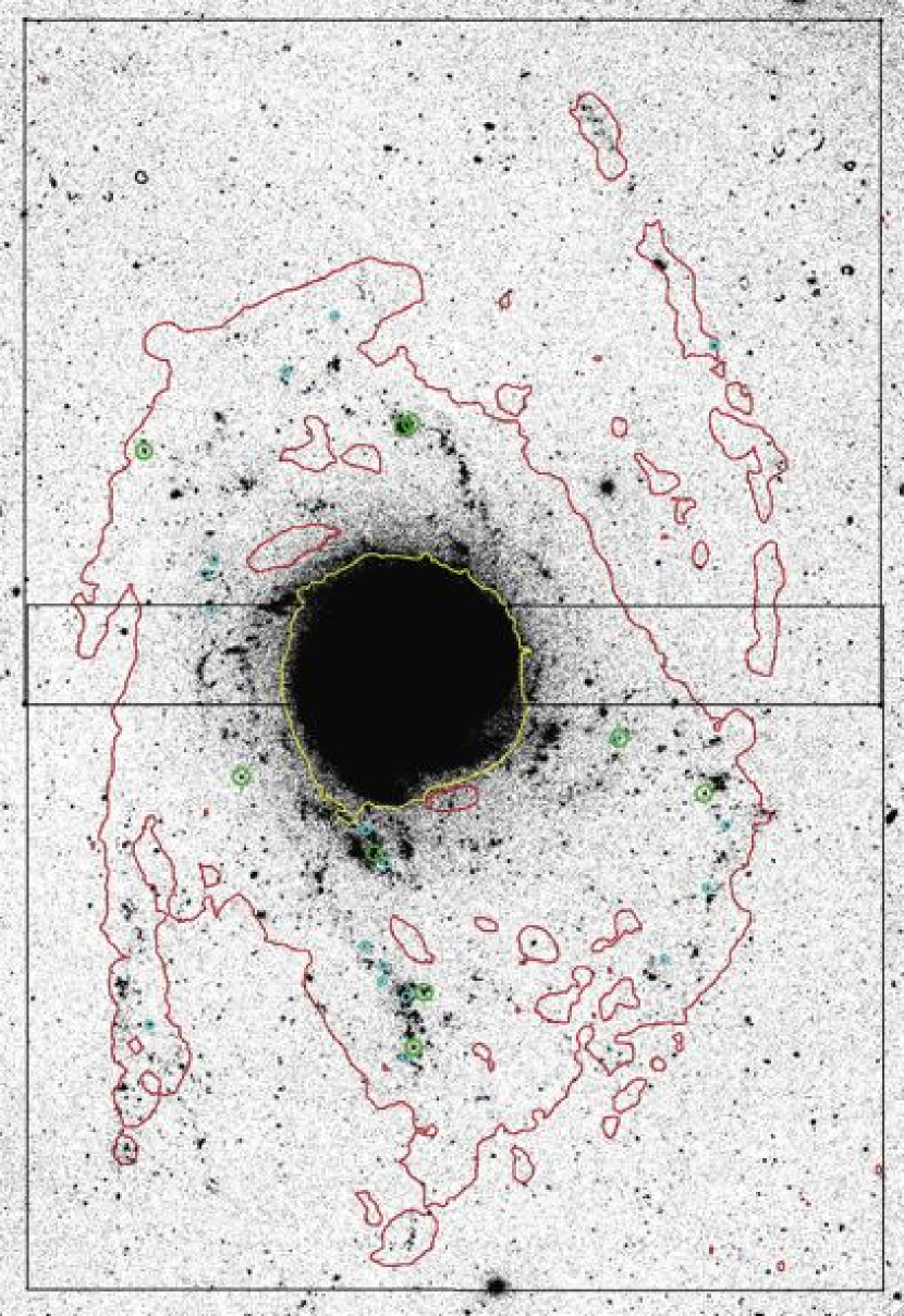
Figure 1.— Subaru coverage and definition of regions in M83. The background is a GALEX FUV image downloaded from Galexview. Solid overlapping rectangles are two pointings with the Subaru Prime Focus Camera (Suprime-Cam; the field-of-view is $34\arcmin\times 27\arcmin$, or $44.5\times 35.3\,\rm kpc^{2}$, in one pointing). The inner (yellow) contour is roughly at the traditional edge of the optical disk. The outer (red) counter is at an HI surface density of $1.5\times 10^{20}\rm\,cm^{-2}$, using the HI data from Miller, Bregman & Wakker (2009). We call FUV-bright objects inside the HI contour IN objects (excluding those in the inner disk - yellow contour), and those outside OUT objects. The H$\alpha$-bright clusters (${\rm NA659}-{\rm R}_{\rm C}<-1$ mag; §4) are also plotted: green for clusters with $>10^{3}{\rm M_{\odot}}$ and cyan for the ones with $<10^{3}{\rm M_{\odot}}$.

2.2. GALEX

We use archival GALEX far-ultraviolet (FUV) and near-ultraviolet (NUV) images (Bigiel et al., 2010). The data are obtained from the GALEX data archive through Galexview in the multimission archive at STScI (MAST). The GALEX observations and data reduction were discussed in Bigiel et al. (2010). The FWHM sizes of the point spread functions (PSF) are measured with the IDL software ATV (Barth, 2001) and are $4.7\arcsec$ for FUV and $5.2\arcsec$ for NUV. The $1\sigma$ photometric limits with the $\sim 5\arcsec$ aperture are 26.34 and 26.20 AB mag in the FUV and NUV-bands, respectively.

3. Methods

3.1. Stellar Population Synthesis Model

Our analysis is guided by the stellar population synthesis model Starburst99 (Leitherer et al., 1999). The Padova stellar evolution tracks with AGB stars are adopted. Most UV-bright objects in the XUV disk of M83 are likely stellar clusters (Thilker et al., 2005; Gil de Paz et al., 2007). Therefore, we adopt an instantaneous burst approximation to model their photometric evolution.

We will show that the standard Salpeter IMF (Salpeter, 1955) explains the observations well. Figure 2 demonstrates the differences between the standard and truncated IMFs. The cluster mass is set to $1000{\rm M_{\odot}}$ for the plot, which is roughly the minimum mass of a cluster to fully populate the IMF up to an O star (see Appendix A). Note that a factor of 10 increase in cluster mass shifts all the magnitude curves in Figure 2 (top) systematically upward by 2.5 magnitudes, but it does not change the color curves. For these models, we assume the Salpeter IMF with a lower cut-off mass of $m_{l}=0.1{\rm M_{\odot}}$. The upper cut-off mass is set to $m_{u}=$ 100, 20, and 3 ${\rm M_{\odot}}$, which corresponds to the masses of the most massive O, B, and A-type stars, respectively (Cox, 2000). In other words, the last two models represent the truncated IMF (or, almost equivalently, the steeper IMF) without O or OB stars. We adopt 20% of the solar metallicity ($0.2{\rm Z_{\odot}}$) from the spectroscopic measurements (Gil de Paz et al., 2007; Bresolin et al., 2009). For a reference, the spectra of individual O, B and A stars are discussed in Appendix B.

There are quantitative differences between clusters with and without OB stars, i.e., between the standard and truncated (steeper) IMFs. Clusters without OB stars are fainter by 6 mag in FUV for the first 10 Myr and never become as blue as FUV-NUV$<$0.2$-$0.3 mag. Therefore, blue clusters ($<$0.2$-$0.3 mag) must have O and/or B stars. The FUV-NUV color is insensitive to the difference between clusters with only B stars (up to $m_{u}=20{\rm M_{\odot}}$) and with both O and B stars ($100{\rm M_{\odot}}$). This is primarily because the GALEX bands trace only the Rayleigh-Jeans side of stellar thermal radiation for both O and early-type B stars (Appendix B). The FUV-NUV color is therefore a useful indicator of the presence of O and/or B stars in a cluster.

The ${\rm NA659}-{\rm R}_{\rm C}$ color differentiates clusters with O stars from those without them, since O stars emit a significantly greater number of ionizing photons than B stars (Sternberg, Hoffmann & Pauldrach, 2003). This is demonstrated in Figure 2 (bottom). Clusters with ${\rm NA659}-{\rm R}_{\rm C}<$ -1 mag must have O stars, and those with ${\rm NA659}-{\rm R}_{\rm C}<$ -0.3 mag should have O and/or B stars. For this plot, we calculated the ${\rm H}{\alpha}$ line luminosity $L_{{\rm H}{\alpha}}$ using the Lyman photon flux $Q_{\rm Lyc}$ from Starburst99 and the relation $L_{{\rm H}{\alpha}}{\rm[erg\,s^{-1}]}=1.37\times 10^{-12}Q_{\rm Lyc}{\rm[s^{-1}]}$ from case B recombination with an electron temperature of $10^{4}$K (Gavazzi et al., 2002). Case B recombination is perhaps a reasonable assumption even in the low-density environment, since the optical depths in the Lyman resonance lines are very likely quite large (Osterbrock & Ferland, 2006) in any star-forming conditions. The ${\rm NA659}$ magnitude is based on the stellar continuum luminosity plus $L_{{\rm H}{\alpha}}$. We ignore the effect of [NII] emission since the effect is very small (Gil de Paz et al., 2007; Kennicutt et al., 2008; Goddard, Kennicutt & Ryan-Weber, 2010, see §4.1).

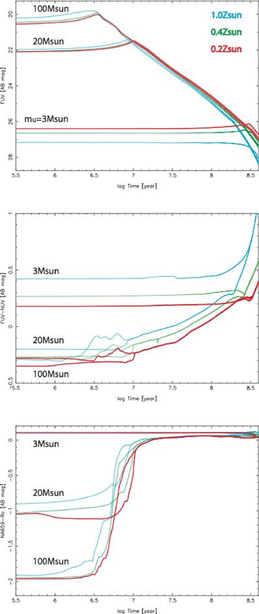
Figure 2.— Photometric evolution of stellar clusters from Starburst99. A single-burst model with the Salpeter IMF is adopted. A low metallicity (0.2 ${\rm Z_{\odot}}$) is adopted (red) for the analysis, but models of higher metalicities (0.4${\rm Z_{\odot}}$ and 1.0${\rm Z_{\odot}}$) are also plotted (green and cyan, respectively). The lower mass boundary for the IMF is $0.1{\rm M_{\odot}}$, and the upper mass boundary is $100{\rm M_{\odot}}$ (including all types of stars), $20{\rm M_{\odot}}$ (no O stars), and $3{\rm M_{\odot}}$ (no OB stars). The adopted distance of M83 is $d=4.5\,{\rm Mpc}$. Top: FUV magnitude for a cluster mass of $1000{\rm M_{\odot}}$. Middle: FUV-NUV color. Bottom: ${\rm NA659}$-$R_{C}$ color.

3.2. Cluster Counts

Counting blue clusters in FUV-NUV and ${\rm NA659}-{\rm R}_{\rm C}$ constrains the IMF at its high mass end. Clusters become bright in ${\rm H}{\alpha}$ (“blue” in the color ${\rm NA659}-{\rm R}_{\rm C}$) predominantly due to O stars, while FUV-NUV is due to both O and B stars. Since O stars have much shorter lives than B stars, ${\rm NA659}-{\rm R}_{\rm C}$ changes faster than FUV-NUV (Figure 2). Under the assumptions of instantaneous cluster formation and a constant cluster formation rate, the numbers of blue clusters in FUV-NUV and ${\rm NA659}-{\rm R}_{\rm C}$ ($N_{\rm UV}$ and $N_{{\rm H}{\alpha}}$) should be proportional to the durations that clusters are blue ($t_{\rm UV}$ and $t_{{\rm H}{\alpha}}$, respectively). Thus, we expect $N_{{\rm H}{\alpha}}/N_{\rm UV}=t_{{\rm H}{\alpha}}/t_{\rm UV}$ if the difference in the populations is due to a simple aging effect starting from the initial populations of the standard IMF. The assumption of a constant cluster formation rate should be approximately accurate when integrated over the large XUV disk and over a short timescale, i.e., the young ages of clusters which can be detected with our color selection criteria (below). In fact, the clusters that we count in §5.3 are distributed over the UV disk (Figure 1).

For the standard IMF ($m_{u}=100{\rm M_{\odot}}$ and $0.2{\rm Z_{\odot}}$), a cluster is blue (e.g., FUV-NUV$<0.0$ mag) for $t_{\rm UV}=70.8$ Myr and ${\rm H}{\alpha}$-bright (e.g., ${\rm NA659}-{\rm R}_{\rm C}<-1.0$ mag) for $5.8$ Myr. Therefore, the number ratio should be $N_{{\rm H}{\alpha}}/N_{\rm UV}=0.08$ if each population is the consequence of the cluster aging effect. We will compare the observations with this theoretical prediction.

We identify and count stellar clusters at the GALEX resolution ($\sim 5\arcsec$; $\sim 109$ pc at the distance of M83). It is possible that clusters may be blended at this resolution; however, even in that case, our analysis is valid if clusters formed in such proximity are typically coeval.

4. Sample Selection

4.1. FUV-Selected Objects

UV-bright objects are identified based on the FUV image using the SExtractor package (Bertin & Arnouts, 1996). Saturated stars and image edges are masked before the identification. Objects within the traditional optical disk (yellow contour in Figure 1) are excluded. We confirmed the very low probability of false detection using the negative image technique. SExtractor is run against the sign-flipped FUV image and detected only one false target at 25.41 mag in FUV. Thus, false detections have a negligible impact on our number counts.

The aperture photometry is carried out in the four bands with the dual image mode of SExtractor using the FUV image as the reference. The $1\sigma$ photometric limits with the aperture of the GALEX resolution ($\sim 5\arcsec$) are 24.90, 25.56, 26.34, and 26.20 mag in the ${\rm NA659}$ (${\rm H}{\alpha}$), $R_{C}$, FUV, and NUV-bands, respectively. The sensitivity in ${\rm NA659}$ (FWHM=120$\rm\AA$) corresponds to a flux of $7.98\times 10^{34}\rm\,erg\,s^{-1}$ at a distance $d=4.5\,{\rm Mpc}$, which is sufficient to detect an HII region around a single B star (e.g., $3.44\times 10^{35}\rm\,erg\,s^{-1}$ in case of B0; assuming case B recombination; see Appendix B). We note that the ${\rm NA659}$ band includes stellar continuum emission as well as ${\rm H}{\alpha}$ emission.

The contamination from [NII]$\lambda 6548$, $6583$ in the ${\rm NA659}$ photometry is neglected. The line ratio [NII]/${\rm H}{\alpha}$ is small ($\lesssim 0.1$) in the outskirts of galaxies (Gil de Paz et al., 2007; Kennicutt et al., 2008; Goddard, Kennicutt & Ryan-Weber, 2010). Even in the extreme case that the stellar continuum has zero contribution to the ${\rm NA659}$ flux, the error is only 0.1 mag (and likely less in more realistic conditions).

Figure 1 shows that the Subaru data cover both the inside and outside of the HI contour (roughly the HI detection limit). Recently-formed FUV-bright objects are more likely to reside inside the HI contour as star formation occurs in gas. For the background subtraction in §4.4, the objects inside the HI contour (hereafter, IN objects) and outside (OUT objects) are separately cataloged. Note that we intensively used the IMCAT software package (Nick Kaiser, private communication) for the following data analysis.

In §5.3, we will discuss a selection of clusters based on their ${\rm NA659}-{\rm R}_{\rm C}$ color; but in advance, Figure 1 shows the locations of clusters with ${\rm NA659}-{\rm R}_{\rm C}<-1$ mag (i.e., bright in ${\rm H}{\alpha}$). They are distributed over the entire XUV disk, and all are within the HI contour (see §4.4).

4.2. Extinction Correction

The extinction curves of Pei (1992) are adopted to correct for Galactic and internal extinctions. The extinctions in FUV, NUV, $R_{\rm C}$, and ${\rm NA659}$ are ($A_{\rm FUV}$, $A_{\rm NUV}$, $A_{R_{\rm C}}$, $A_{{\rm NA659}}$) = (2.58, 2.83, 0.81, 0.81)$A_{\rm V}$ for the Galaxy, (3.37, 2.61, 0.80, 0.80)$A_{\rm V}$ for the Large Magellanic Cloud (LMC), and (4.18, 2.59, 0.79, 0.79)$A_{\rm V}$ for the Small Magellanic Cloud (SMC), where $A_{\rm V}$ is the extinction in $V$-magnitude. We note that the FUV-NUV color becomes bluer under the Galactic extinction, but redder under the LMC and SMC extinction.

The Galactic extinction correction is made for all objects using $A_{\rm V}=0.218$ mag (Schlegel et al., 1998). We do not apply an internal extinction correction until §5, but it will be corrected using $A_{\rm V}=0.1$ mag and the SMC extinction curve for the following reason. The measured metallicity of most outer objects is low ($\sim 0.2{\rm Z_{\odot}}$; Gil de Paz et al., 2007), and therefore, the extinction curve of the SMC is perhaps the most appropriate. Using $E(B-V)$ values from Gil de Paz et al. (2007), we estimate the amount of internal extinction to be around $A_{\rm V}\sim 0.1$ mag with outliers (e.g., 0.0 - 1.0 mag). We therefore adopt $A_{\rm V}\sim 0.1$ mag for the statistical correction, and this degree of extinction will be supported by a comparison with a model color in §5.2.

4.3. Completeness

The mass detection limit is determined in color magnitude space with the help of models. Figure 3 shows color-magnitude diagrams for IN objects. The overlaid solid lines are the 3$\sigma$ and 5$\sigma$ magnitude detection limits and model evolutionary sequences for clusters with masses of $10^{2}$, $10^{3}$, and $10^{4}{\rm M_{\odot}}$. The models are for clusters with the standard Salpeter IMF with ($m_{l}$, $m_{u}$) = (0.1, 100${\rm M_{\odot}}$) and metallicity $0.2{\rm Z_{\odot}}$. Models with lower $m_{u}$ do not reproduce clusters as blue as observed (Figure 2; and see discussion below). Clearly, the mass detection limit changes as a function of color in Figure 3; it decreases as clusters become redder. We note that the ${\rm R}_{\rm C}$ and ${\rm NA659}$ bands are practically at the same wavelength, and therefore, ${\rm NA659}-{\rm R}_{\rm C}$ is zero without ${\rm H}{\alpha}$ emission. A negative ${\rm NA659}-{\rm R}_{\rm C}$ color indicates the presence of associated ${\rm H}{\alpha}$ emission.

The top panel shows that the Subaru observations detect clusters down to $\sim 10^{2}{\rm M_{\odot}}$. Clusters become redder and fainter as they age, and those around the detection boundary ($10^{2}{\rm M_{\odot}}$) become too faint when they become redder than ${\rm NA659}-{\rm R}_{\rm C}\sim-0.6$ mag. In other words, the sample is complete down to $10^{2}{\rm M_{\odot}}$ in the range ${\rm NA659}-{\rm R}_{\rm C}<-0.6$ mag. It is complete down to $10^{3}{\rm M_{\odot}}$ in ${\rm NA659}-{\rm R}_{\rm C}<0.0$ mag. The extinction is negligible, as shown by the extinction vector (for $A_{\rm V}=0.1$ mag) in the plot.

The bottom panel shows the corresponding color-magnitude diagram in the UV. Again, the mass detection limit is a function of the color range (and thus, the cluster age). The detection limit is $\sim 10^{3}{\rm M_{\odot}}$ for the color FUV-NUV$<0.0$ mag and is even deeper ($\sim 10^{2}{\rm M_{\odot}}$) for FUV-NUV$<-0.2$ mag. The extinction is not negligible in FUV and NUV and will be discussed later.

Note that the very blue objects in the bottom panel (FUV-NUV$\lesssim-0.3$ mag and FUV $\sim 22$ - 24 mag) are bluer than any model cluster with the standard IMF can reproduce, and are located approximately in the region where single O stars appear (the models of O3 and B0 stars are also plotted). These objects are not included in our number count, since they appear below the mass selection criterion in §5.3. We will discuss these objects in §5.1.

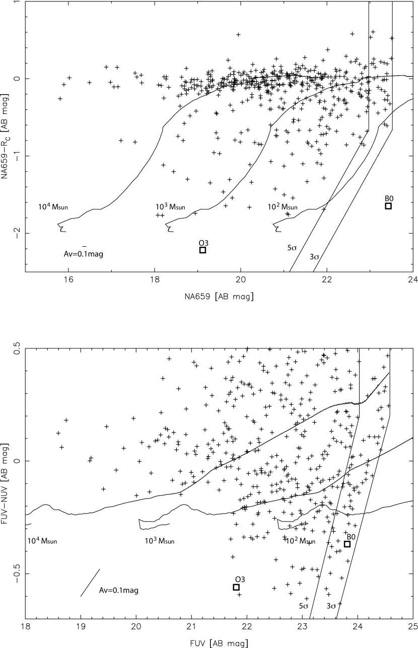
Figure 3.— Color-magnitude diagrams of all the objects inside the HI contour (IN objects defined in §4.1). Top: ${\rm NA659}$-${\rm R}_{\rm C}$ vs ${\rm NA659}$. $5\sigma$ and $3\sigma$ detection limits are illustrated with solid straight lines. The model evolutionary sequences with the standard Salpeter IMF are displayed with solid curves for clusters with $10^{2}$, $10^{3}$, $10^{4}{\rm M_{\odot}}$. Bottom: The same as the top panel, but for FUV-NUV vs FUV. Single O3 and B0 star models are also plotted in both panels.

4.4. Background Subtraction

The contamination of background (and foreground) objects has been an obstacle in identifying the objects within nearby galaxies (Werk et al., 2010; Goddard, Kennicutt & Ryan-Weber, 2010). The large field-of-view of Suprime-Cam is a clear advantage as it enables us to remove such contamination statistically. The objects outside the HI gas contour (OUT objects; see §4.1) are most likely in the background, whereas IN objects include stellar clusters within M83 as well as background objects.

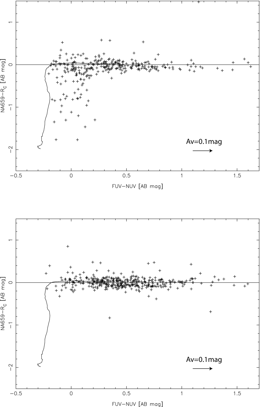
Figure 4.— ${\rm NA659}$-${\rm R}_{\rm C}$ vs FUV-NUV color-color plot of the objects above $5\sigma$-detection and above $10^{3}{\rm M_{\odot}}$. Lines are model predictions with the Salpeter IMF with $m_{u}=100{\rm M_{\odot}}$ for 0.2 ${\rm Z_{\odot}}$. A reddening vector of $A_{\rm V}=0.1$ mag from the SMC extinction curve is also plotted. We assume that stellar clusters (traced in ${\rm R}_{\rm C}$) and the surrounding ionized gas (in ${\rm NA659}$) suffer from extinction by the same amount. Top: FUV-bright objects within the HI contour (IN objects). Bottom: the FUV-bright objects outside (OUT objects).

The IN and OUT objects show different colors statistically. Figure 4 shows the plots of ${\rm NA659}$-${\rm R}_{\rm C}$ vs FUV-NUV for the IN and OUT objects above the $5\sigma$ magnitude detection limit and above the $10^{3}{\rm M_{\odot}}$ threshold line in Figure 3 (bottom). Figure 5 is a histogram of FUV-NUV color for the IN (green) and OUT objects (blue). Clearly, the IN objects are bluer in FUV-NUV than the OUT objects and preferentially have FUV-NUV$<$0.2$-$0.3 mag, while the OUT objects are more likely to have FUV-NUV$>$0.2$-$0.3 mag. Figure 4 shows that virtually all objects with ${\rm NA659}-{\rm R}_{\rm C}$ $<$ -0.3 mag (OB stars) are IN objects; almost no young stellar clusters exist outside of the HI gas. This clear distinction ensures that the objects outside of the HI gas are not the young clusters in M83 and represent the background population. Note that IN objects are young stellar clusters, not very old clusters with many evolved FUV-bright stars, such as extreme horizontal branch stars, blue stragglers or planetary nebulae. The old clusters do not become as blue in FUV-NUV as our IN objects (Donovan et al., 2009).

The background contamination in the IN objects can be removed statistically; we subtract the OUT objects from the IN. In Figure 5 the number of the OUT objects are scaled by the IN/OUT area ratio (55%) and subtracted from that of the IN objects. The derived histogram (red) represents the population of young clusters with mass $>10^{3}{\rm M_{\odot}}$ in the XUV disk.

Virtually all clusters after the subtraction show blue color in FUV-NUV ($<$ 0.2$-$0.3 mag; Figure 5), suggesting that all of these young clusters have O or, at least, B stars (see Figure 2). Thus, massive stars are populated even in the diffuse gas environment. It is also remarkable that almost no red objects (FUV-NUV $>$0.2$-$0.3 mag) exist. This confirms that OUT objects are distributed everywhere across our field-of-view and represent the background objects; thus, our background subtraction is fairly successful.

There is a possibility that old stellar clusters (i.e., FUV-NUV $>$0.2$-$0.3 mag before extinction correction) exist both in the IN and OUT regions and are removed from the IN population. However, it should not affect our cluster count analysis as we discuss only the young clusters. Such a population, if it exists, must be fairly uniformly distributed both in the IN and OUT regions, since the count after the subtraction is nearly zero in FUV-NUV $>$0.2$-$0.3 mag. We also note that the apparent magnitudes of low mass clusters ($\lesssim 10^{3}{\rm M_{\odot}}$) fall below our detection limit after $\sim 100$ Myr (Figure 2 top). Again, this is not a problem with the selection criteria that are adopted in our analysis (§5.3).

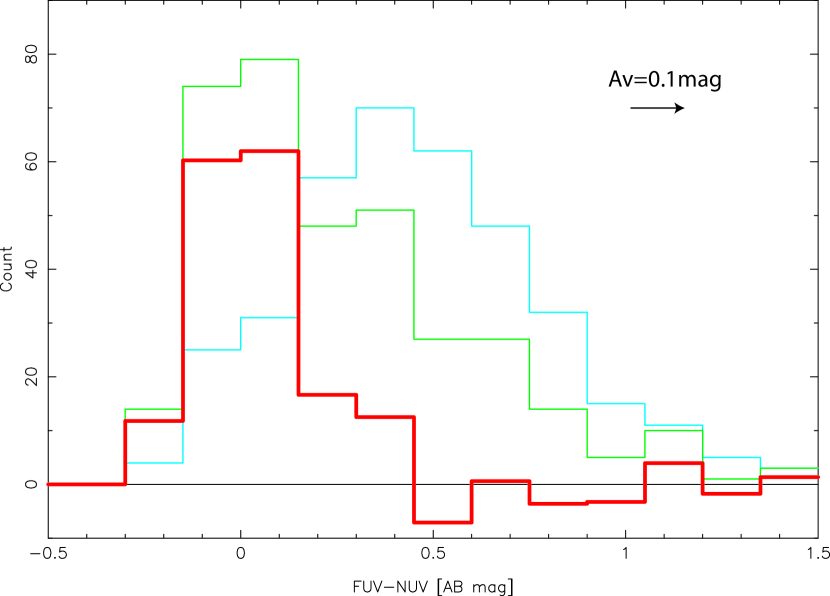
Figure 5.— Histograms of FUV-NUV color of the objects above $5\sigma$-detection and above $10^{3}{\rm M_{\odot}}$. Colors indicate the objects within the HI gas (green), the ones outside of the HI gas (background objects; blue), and the ones associated with M83 (red). The associated ones are calculated by subtracting OFF from ON with scaling for the area coverage difference.

5. Discussion

5.1. Truncated vs Stochastic IMFs

The presence of ionizing stars (O stars) is evident even in small clusters ($<10^{3}{\rm M_{\odot}}$) in Figure 3, suggesting that the IMF is not truncated. Massive stars do not form under the truncated IMF at all. On the other hand, they should appear occasionally even in small clusters under the stochastic IMF, though they tend not to appear in a small sample due to their low probability of formation in small clusters. Such a stochastic effect becomes particularly apparent when the cluster mass is small ($<1000{\rm M_{\odot}}$). Our Subaru observations detect small clusters (down to $\sim 10^{2}{\rm M_{\odot}}$) and confirm that even those small clusters show ${\rm H}{\alpha}$ excess (i.e., ${\rm NA659}-{\rm R}_{\rm C}<0.0$ mag); and some even have ${\rm NA659}-{\rm R}_{\rm C}<-1.0$ mag, a color which only O stars can produce. Thus, O stars are present in the $10^{2-3}{\rm M_{\odot}}$ clusters. The IMF is not truncated even in the low-density and low-metallicity environment.

More precisely, it is necessary to account for the stochastic effects in discussions of very low mass clusters ($<10^{3}{\rm M_{\odot}}$) – and even then, our result still supports the stochastic IMF over the truncated IMF, as we discuss below. We first need to consider the likelihood that a cluster with a given small mass has a massive star. In Appendix A we estimate that a $10^{3}{\rm M_{\odot}}$ cluster is likely to have as massive star as $40{\rm M_{\odot}}$; the cluster mass must be greater than $\sim 400{\rm M_{\odot}}$ to have a high probability of hosting at least one O star ($>20{\rm M_{\odot}}$); a $10^{2}{\rm M_{\odot}}$ cluster likely hosts up to a $\sim 10{\rm M_{\odot}}$ star.

The ${\rm NA659}-{\rm R}_{\rm C}$ color is sensitive to the mass of the most massive star in a cluster when the cluster is young, whereas FUV-NUV does not distinguish O stars from B stars well (§3.1; Figure 2; see also Appendix B). If a cluster has no massive star, it should appear redder (${\rm NA659}-{\rm R}_{\rm C}>$ -1 mag; Figure 2) than the observed clusters in the range $10^{2-3}{\rm M_{\odot}}$; yet some clusters appear in the range ${\rm NA659}-{\rm R}_{\rm C}=$ -1$\sim$ -2 mag. Massive O stars in small clusters should be populated stochastically. In addition, a stochastically-populated single O star can outshine a cluster with a small mass ($10^{2-3}{\rm M_{\odot}}$; Figure 2). This may result in an overestimation of the cluster mass when we apply the standard IMF with $m_{u}=100{\rm M_{\odot}}$ to the cluster (as done in Figure 3). Therefore, the masses of small clusters that appear in the range $10^{2-3}{\rm M_{\odot}}$ in Figure 3 could be actually even less. This prefers the stochastic IMF, as even the less massive clusters have O stars.

The discussion so far is about clusters of stars. Another possible evidence for the presence of O stars is the population of very blue objects (FUV-NUV$\lesssim-0.3$ mag) in Figure 3 (bottom). They have the apparent magnitude and color similar to those of a single O star. They are possibly isolated, single O stars or small clusters with an O star(s) but without many low-mass stars. Higher resolution images are necessary to confirm them; their presence, if confirmed, may be stronger evidence for O stars that are formed in the low-density environments.

5.2. Internal Extinction Correction

The internal extinction is assumed to be $A_{\rm V}=0.1$ mag from spectroscopic measurements (§4.2; Gil de Paz et al., 2007). This degree of extinction on average is also supported by a comparison with the model curve in Figure 4 (top). The extinction vector, corresponding to $A_{\rm V}=0.1$, is also plotted. An extinction correction by this amount creates agreement between the UV data and the model curve, providing additional support for the adopted $A_{\rm V}$.

We assume that a stellar cluster (traced in ${\rm R}_{\rm C}$) and the surrounding ionized gas (in ${\rm NA659}$) suffer from extinction by the same amount. The two components may have different spatial distributions and a slightly different attenuation (e.g., $E(B-V)_{\rm continuum}\sim 0.44E(B-V)_{\rm gas}$ in case of more active star-forming environments; Calzetti, 2001). However, the difference is negligible for our analysis since the extinction is small ($A_{\rm V}=0.1$).

5.3. Universal IMF

Detected clusters with a color of ${\rm NA659}-{\rm R}_{\rm C}<-1$ mag are evidence that some clusters host O stars. Here we test whether their abundance, relative to the ones without O stars, can be explained by a simple aging effect with the standard IMF. Under the assumptions of instantaneous formation of star clusters and a constant cluster formation rate over the XUV disk, the numbers and durations of blue clusters should show the relation $N_{{\rm H}{\alpha}}/N_{\rm UV}=t_{{\rm H}{\alpha}}/t_{\rm UV}$, if the relative cluster populations are due to the aging effect.

Consistent sample selection between GALEX and Subaru data is crucial in this analysis. Each of the four photometric bands has its own detection limit (Figure 3), and a bias could be introduced if only magnitude detection limits are taken into account. We therefore use the cluster mass and color as thresholds for cluster counts. As discussed in §4.3, both GALEX and Subaru data are complete at $\gtrsim 5\sigma$, in colors ${\rm NA659}-{\rm R}_{\rm C}<-0.3$ mag and FUV-NUV$<0.0$ mag down to a cluster mass $10^{3}{\rm M_{\odot}}$. This is true even after the internal extinction correction (§5.2) if a slightly lower detection limit ($3.4\sigma$) is adopted. The extinction correction is made for all four bands, which is equivalent to shifting the data points along the extinction vectors in Figure 3. We select the mass limited sample after the extinction correction using the technique discussed in §4.

Almost all of the clusters are in the range FUV-NUV $<$ 0 mag when the extinction is taken into account (Figure 5); thus, we adopt this color range for our analysis. This is the range where B stars definitely, and O stars possibly, exist in the clusters; we count how many of them have O stars below. Clusters are blue, FUV-NUV$<0$ mag, for only a short duration. With the standard IMF of $(m_{l},m_{u})=(0.1,100{\rm M_{\odot}})$ and $0.2{\rm Z_{\odot}}$, this is $t_{\rm UV}=71$ Myr (Figure 2). The short $t_{\rm UV}$ is advantageous, since the assumption of a constant cluster formation rate is likely valid for a short period over the large area (i.e., the entire XUV disk) – no local events likely bias the statistics. On the other hand, clusters with O stars show ${\rm NA659}-{\rm R}_{\rm C}<-1$ mag for only 5.8 Myr. The model therefore predicts $t_{\rm{\rm H}{\alpha}}/t_{\rm UV}\sim 0.08$.

The number of blue clusters with FUV-NUV $<$ 0 mag is counted using Figure 5 (red) – after the internal extinction correction, it is $N_{\rm UV}=88\pm 9$. From Figure 3, $N_{{\rm H}{\alpha}}=9\pm 3$ for ${\rm NA659}-{\rm R}_{\rm C}<-1$ mag (see Figure 6). The errors are based on the Poisson distribution, and the counts are made after the internal extinction correction. Therefore, the observed ratio is $N_{{\rm H}{\alpha}}/N_{\rm UV}\sim 0.10\pm 0.03$. This is consistent with the prediction of the standard IMF (within a 1$\sigma$ deviation). The counts of stellar clusters support the standard IMF with a simple aging effect.

It is worth noting that the slight deviation does not likely have a statistical significance. However, if anything, it is inclined toward the top-heavy IMF side, as opposed to the previous suggestion of a truncated IMF.

The combination of the parameters we adopt [i.e., low metallicity ($0.2{\rm Z_{\odot}}$), SMC extinction, and $A_{\rm V}=0.1$ mag] is the best to consistently explain the new data, model, and previous spectroscopic studies. The result for the standard IMF does not change even if a higher metallicity ($\sim 0.4{\rm Z_{\odot}}$), and hence the LMC extinction curve, is adopted. If we ignore the spectroscopic studies, the comparison of the data and model (e.g., Figure 4) provides $A_{\rm V}\sim 0.2$ mag. With this extinction, we count $N_{\rm UV}=86\pm 9$ and $N_{{\rm H}{\alpha}}=11\pm 3$ and obtain $N_{{\rm H}{\alpha}}/N_{\rm UV}\sim 0.13\pm 0.04$. The model ratio is 0.10 with the metallicity $0.4{\rm Z_{\odot}}$, where $t_{\rm{\rm H}{\alpha}}=5.2$ Myr and $t_{\rm UV}=51.3$ Myr. Therefore, the observations and model are consistent even if a different metallicity and extinction are assumed.

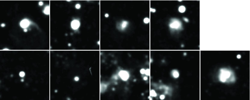
Figure 6.— ${\rm NA659}$ images of the ${\rm H}{\alpha}$-bright clusters with ${\rm NA659}-{\rm R}_{\rm C}<-1$ mag and $>10^{3}{\rm M_{\odot}}$. O-type stars must be present to produce this cluster color. The size of each image is $24\arcsec.2\times 24\arcsec.2$.

5.4. ${\rm H}{\alpha}$-to-FUV Flux Ratio

The ${\rm H}{\alpha}$-to-FUV flux ratio ($F_{{\rm H}{\alpha}}/f_{\nu\,\rm FUV}$) over the entire XUV disk is another measure of the high-mass end of the IMF. We find that the observed ratio is consistent with the one predicted from the standard IMF. A lower ratio may suggest a truncated IMF (Meurer et al., 2009; Lee et al., 2009), though an extinction correction introduces an ambiguity (Boselli et al., 2009). We can estimate the ratio more accurately since we derived the extinction of $A_{\rm V}=0.1$ mag statistically (§5.2).

In a Starburst99 simulation with a constant star formation rate, a metallicity of $0.2{\rm Z_{\odot}}$, and the Salpeter IMF with ($m_{\rm l}$, $m_{\rm u}$) = (0.1, 100)${\rm M_{\odot}}$, the ratio approaches an approximate constant and is, e.g., $\log(F_{{\rm H}{\alpha}}/f_{\nu\,\rm FUV})\sim 13.10$ in unit of $\log({\rm Hz})$ after 1 Gyr assuming a star formation rate of $\rm 1{\rm M_{\odot}}/yr$ (though the constant does not depend on these values). Fumagalli, da Silva & Krumholz (2011) calculate the ratio with their own model using the Kroupa IMF and derive $\sim 13.22$ (from their Figure 1). The scatter between the models is about 30%. Compared to these values, the observed ratios previously reported in LSB galaxies by Meurer et al. (2009) – as low as one third of the values calculated in these models – deviate at a significant level with respect to the model uncertainties.

We calculate the ${\rm H}{\alpha}$ to FUV flux ratio over the XUV disk of M83 by summing up the fluxes of all $>3\sigma$ detections in the FUV image (§4.1). Assuming that OUT objects represent the background population (§4.4) and subtracting their total fluxes form those of IN objects (accounting for the IN/OUT area ratio), we obtain $F_{{\rm H}{\alpha}}=8.36\times 10^{28}\,\rm erg\,s^{-1}$ and $f_{\nu\,\rm FUV}=7.23\times 10^{25}\,\rm erg\,s^{-1}\,Hz^{-1}$. Adopting $A_{\rm V}=0.1$ mag and the SMC extinction curve (§4.2), the intrinsic ratio after the extinction correction is $\log(F_{{\rm H}{\alpha}}/f_{\nu\,\rm FUV})_{\rm int}=12.93$. This value is only $\sim 30\%$ lower than our model prediction, and not as much as what the previous study found (Meurer et al., 2009). As the difference between this value and our model calculation is similar to the scatter between the models, we consider a truncated IMF to be unwarranted in the case of M83.

6. Summary

Using new deep Subaru ${\rm H}{\alpha}$ data and archival GALEX data of the extended ultraviolet (XUV) disk of M83, we show that the standard Salpeter IMF explains the number counts of stellar clusters in the low density, low metallicity environment. Even in clusters with small mass ($10^{2-3}{\rm M_{\odot}}$) O stars are populated, at least occasionally, suggesting that the stochastic IMF is preferable to the truncated IMF. The ${\rm H}{\alpha}$ to FUV flux ratio over the XUV disk also supports the standard IMF.

The analyses were guided by the stellar population synthesis model Starburst99. The new data, together with the population synthesis model and previous spectroscopic studies, provide overall very consistent results at the metallicity ($\sim 0.2{\rm Z_{\odot}}$), internal extinction ($A_{\rm V}\sim 0.1$ mag), and colors of the stellar clusters in the XUV disk. We counted the numbers of FUV-bright clusters (which should have O and/or B stars) and ${\rm H}{\alpha}$-bright clusters (having O stars), whose ratio constrains the high-mass end of the IMF. The ratio of number counts can be translated to the ratio of their lifetimes with Starburst99, under the two assumptions of instantaneous cluster formation and a constant cluster formation rate in the XUV disk. As a result, the number counts are consistent with the Standard IMF and a simple aging effect.

This study benefits from the combination of the unparalleled wide field-of-view and sensitivity of Suprime-Cam. The new image covers an area far beyond the detection limit of the HI gas (thus, beyond the boundary of the XUV disk), enabling us to remove the background contaminations statistically, which had been a difficulty in previous studies. We found that virtually all blue clusters (FUV-NUV$\lesssim$ 0.0 mag after the extinction correction; or $\lesssim$ 0.16 mag before the correction) are within the HI gas.

Appendix A Minimum stellar cluster mass to avoid stochasticity

We consider the threshold mass of a stellar cluster where the incomplete sampling (filling) of the IMF (i.e., stochastic effect) becomes important. It depends on the definition of “stochastic sampling”, because in reality an O star with the highest mass $\sim 100{\rm M_{\odot}}$ is rarely found (at least in the Milky Way), and even a massive cluster (e.g., $10^{6}{\rm M_{\odot}}$) may not host any star with $100{\rm M_{\odot}}$ in a statistical sense. On the contrary, we could define the fully-sampled IMF as the one in which at least one O star of any subclass ($>20{\rm M_{\odot}}$) is populated. Of course, a cluster is more likely to host a $20{\rm M_{\odot}}$ star than a $100{\rm M_{\odot}}$ star, and the threshold mass should be lower in the former case. One could also take a different approach; for example, Calzetti et al. (2010) found $\sim 10^{3}{\rm M_{\odot}}$ as the threshold mass where the ${\rm H}{\alpha}$ luminosity over cluster mass starts to deviate from a constant.

Here, we take a simpler approach to illustrate a range of threshold cluster mass that may provide an important guideline. The threshold mass necessary to populate the IMF to some upper mass cutoff depends on that maximum stellar mass

The stellar initial mass function ($\Psi(m)$) with the upper and lower stellar mass cuts ($m_{u}$ and $m_{l}$, respectively) is normalized as

$$M_{\rm cl}=\int^{m_{u}}_{m_{l}}m\Psi(m)dm,$$ (A1)

where $M_{\rm cl}$ is the total mass of a stellar cluster. Assuming a power-law IMF ($\Psi(m)=Am^{-\alpha}$) the normalization coefficient ($A$) is

$$A=M_{\rm cl}\frac{2-\alpha}{m_{u}^{2-\alpha}-m_{l}^{2-\alpha}}.$$ (A2)

If we sum up the masses of all stars with masses greater than a threshold stellar mass $m_{t}$, the sum is

$$M(>m_{t})=\int^{m_{u}}_{m_{t}}m\Psi(m)dm.$$ (A3)

In order to populate at least one star as massive as $m_{t}$, this sum should be greater than $m_{t}$ [i.e., $M(>m_{t})>m_{t}$]; and therefore,

$$M_{\rm cl}>m_{t}\frac{m_{u}^{2-\alpha}-m_{l}^{2-\alpha}}{m_{u}^{2-\alpha}-m_{t}^{2-\alpha}}$$ (A4)

in the case of a power-law IMF. This condition is necessary to unstochastically populate the IMF up to $m_{t}$ in the cluster, providing a threshold cluster mass to have a star up to mass $m_{t}$.

A similar calculation also provides a guideline of the maximum stellar mass that a cluster with $M_{\rm cl}$ is likely to host – the IMF would be filled up to $m_{t}$ if it is populated smoothly from the lowest stellar mass $m_{l}$ toward the highest until the total mass reaches the cluster mass $M_{\rm cl}$. Thus, the maximum stellar mass in the cluster is around $m_{t}$.

Figure 7 shows the threshold cluster mass $M_{\rm cl}$ as a function of the maximum stellar mass $m_{t}$ that should be populated. We assumed the Salpeter IMF ($\alpha=2.35$), $m_{l}=0.1{\rm M_{\odot}}$, and $m_{u}=100{\rm M_{\odot}}$. In order to have a $40{\rm M_{\odot}}$ star the cluster mass should be at minimum $10^{3}{\rm M_{\odot}}$, while to have $80{\rm M_{\odot}}$ it needs to be $10^{4}{\rm M_{\odot}}$. All stars with $>20{\rm M_{\odot}}$ are classified as O-type stars; and to have at least one O star the cluster mass should be greater than $\sim 400{\rm M_{\odot}}$. To fill the IMF literally up to $\sim 100{\rm M_{\odot}}$, the cluster mass should be on the order of $10^{5}{\rm M_{\odot}}$. If we adopt $50{\rm M_{\odot}}$ (arbitrarily) as a typical mass of O stars, the cluster mass should be $>2000{\rm M_{\odot}}$ to fully populate the IMF up to this typical O star mass and avoid the stochastic effect.

These threshold cluster masses are meaningful only in a statistical sense. A stochastic effect could appear even above this threshold mass if a Monte-Carlo simulation is performed. Even if a cluster mass is above the threshold and the cluster can host a star with $m_{t}$, this mass could be split and allocated to multiple stars with smaller masses (whose total is $m_{t}$). On the other hand, a cluster with mass below the threshold could occasionally have a star with mass $>m_{t}$ at the expense of many less massive stars. The threshold cluster mass should be taken as a minimum mass to avoid the stochastic effect, only in a statistical sense. Despite this limitation, our estimate provides a crude guideline for discussion of the stochastic sampling of the IMF.

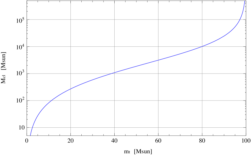
Figure 7.— Minimum cluster mass to avoid the stochastic sampling effect of the IMF, as a function of the maximum stellar mass that one wants to populate unstochastically. The cluster mass needs to be $10^{3}$, $10^{4}$, and a few $10^{5}{\rm M_{\odot}}$ to populate an O star up to 40, 80, 100${\rm M_{\odot}}$, respectively.

Appendix B UV Spectra of O, B and A stars

The spectra of O3, B0, and A0-type stars from the Kurucz’s Atlas9 grid (Kurucz, 1992) are plotted in Figure 8. The masses of these stars are approximately 87.6, 17.5, and 2.9${\rm M_{\odot}}$, respectively (Sternberg, Hoffmann & Pauldrach, 2003; Cox, 2000). We adopt a metallicity of $\rm[Fe/H]=-0.5$ (or $\sim 0.3{\rm Z_{\odot}}$) which is available in the grid. The effective temperature ($T_{\rm eff}$) and gravity ($\log g$) are required to find a model from the grid, and the stellar radius $R$ is necessary to calculate the total flux. From the Atlas9 grid, we choose the models whose parameter sets are the closest to the stellar parameters presented in Sternberg, Hoffmann & Pauldrach (2003) or Cox (2000): ($T_{\rm eff}$, $\log g$, $R$) = (50000 K, 5.0, 13.2 ${\rm R_{\odot}}$), (30000, 4.0, 7.4), and (10000, 4.0, 2.4) for O3, B0, and A0, respectively. We note that the spectra of high-mass stars are not calibrated very well as only few of those exist in the solar neighborhood for calibration. In addition, an adjustment of the parameters is necessary to fit observed spectra of individual stars (Sternberg, Hoffmann & Pauldrach, 2003; Leitherer et al., 2010). The spectra that we present here are only a reference to understand our observations.

The continuum slopes are more or less the same between the O and B stars in the wavelength range of GALEX bands. On the other hand, the A star spectrum is rising from FUV to NUV. The FUV absolute magnitude (AB) and FUV-NUV color of the individual stars for three metallicity [Fe/H]=+0.0 ($1.0{\rm Z_{\odot}}$), -0.5 ($0.3{\rm Z_{\odot}}$), -1.0 ($0.1{\rm Z_{\odot}}$) are in Table 1. We also list the Lyman continuum photon emission rate ($Q_{\rm Lyc}$), which can be used to calculate an H$\alpha$ luminosity ($L_{{\rm H}{\alpha}}{\rm[erg\,s^{-1}]}=1.37\times 10^{-12}Q_{\rm Lyc}{\rm[s^{-1}]}$ in case B recombination). The $Q_{\rm Lyc}$ is calculated by integrating the model spectra over the frequency above the ionizing frequency (i.e., the wavelength of $912\AA$). These $Q_{\rm Lyc}$ values are 4-5 times smaller than those in Sternberg, Hoffmann & Pauldrach (2003), reflecting the uncertainty in model spectra of high-mass stars.

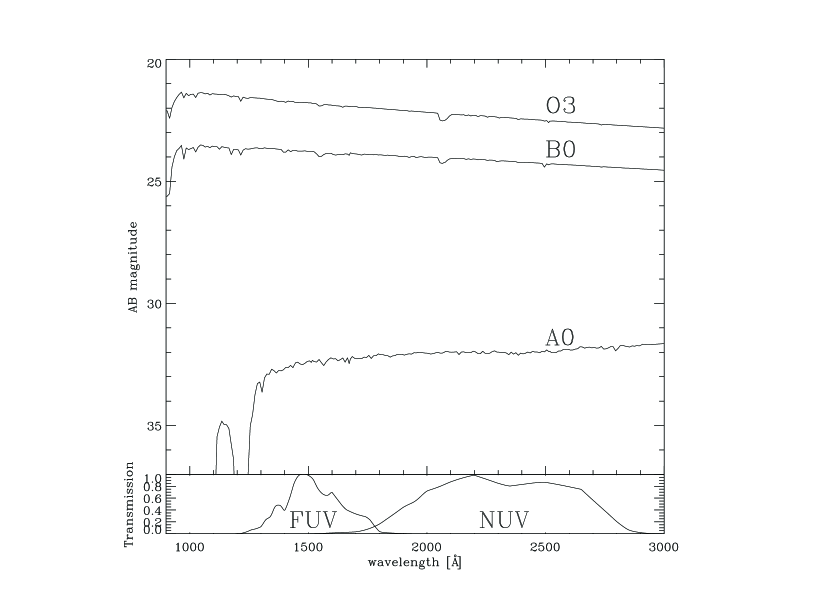
Figure 8.— Top: UV spectra of O3 ($87.6{\rm M_{\odot}}$), B0 ($17.5{\rm M_{\odot}}$) and A0 ($2.9{\rm M_{\odot}}$) stars. The $y$-axis is an apparent magnitude at the distance of M83 ($d=4.5{\rm\,Mpc}$; $m-M$=28.27 mag). Bottom: transmission curves of GALEX FUV and NUV bands.

Table 1UV Color of High-mass Star Models

		$\rm[Fe/H]=+0.0$			-0.5			-1.0
Type	$\log Q_{\rm Lyc}$	FUV	FUV-NUV		FUV	FUV-NUV		FUV	FUV-NUV
	($\rm s^{-1}$)	(mag)	(mag)		(mag)	(mag)		(mag)	(mag)
O3	49.16	-6.47	-0.54		-6.46	-0.57		-6.44	-0.58
B0	47.37	-4.44	-0.31		-4.47	-0.37		-4.48	-0.41
A0	37.24	4.30	0.58		4.16	0.45		4.10	0.40

Note. — FUV magnitudes are the absolute magnitude.

References

- Bakos & Trujillo (2008) Bakos, J. & Trujillo, I. 2008, ApJ, 683, 103
- Barth (2001) Barth, A. J. 2001, in ASP Conf. Ser., Vol. 238, Astronomical Data Analysis Software and Systems X, eds. F. R. Harnden, Jr., F. A. Primini, & H. E. Payne (San Francisco: ASP), 385
- Bastian, Covey & Meyer (2010) Bastian, N., Covey, K. R. & Meyer, M. R. 2010, ARA&A, 48, 339
- Bertin & Arnouts (1996) Bertin, E. & Arnouts, S. 1996, A&AS, 317, 393
- Bigiel et al. (2010) Bigiel, F., Leroy, A., Seibert, M., Walter, F., Blitz, L., Thilker, D. & Madore, B. 2010, ApJ, 720, 31
- Boissier et al. (2007) Boissier, S. et al. 2007, ApJS, 173, 524
- Boselli et al. (2009) Bosellil, A., Boissier, S., Cortese, L. et al. 2009, ApJ, 706, 1527
- Bresolin et al. (2009) Bresolin, F., Ryan-Weber, E., Kennicutt, R. C. & Goddard, Q. 2009, ApJ, 695, 580
- Cox (2000) Cox, A. 2000 ”Allen’s astrophysical quantities”, AIP press.
- Calzetti (2001) Calzetti, D. 2001, New Astronomy Review, 44, 9
- Calzetti et al. (2010) Calzetti, D., Chandar, R., Lee. J. C. et al. 2010, ApJ, 719, 158
- Donovan et al. (2009) Donovan, J. L., Serra, P., van Gorkom, J. H., Trager, S. C., Oosterloo, T., et al. 2009, AJ, 137, 5037
- Ferguson et al. (1998) Ferguson, A. M. N., Wyse, R. F. G., Gallagher, J. S. & Hunter, D. A. 1998, ApJ, 506, 19
- Fumagalli, da Silva & Krumholz (2011) Fumagalli, M., da Silva, R. L. & Krumholz, M. R. 2011, ApJ, 741, 26
- Gavazzi et al. (2002) Gavazzi, G., Bonfanti, C., Sanvito, G., Boselli, A. & Scodeggio, M. 2002, ApJ, 576, 135
- Gil de Paz et al. (2005) Gil de Paz, A., Madore, B. F., Boissier, S., Swaters, R., Popescu, C. C., Tuffs, R. et al. 2005, ApJ, 627, 29
- Gil de Paz et al. (2007) Gil de Paz, A., et al. 2007, ApJ, 661, 115
- Goddard, Kennicutt & Ryan-Weber (2010) Goddard, Q. E., Kennicutt, R. C. & Ryan-Weber, E. V. 2010, MNRAS, 405, 2791
- Hayashino et al. (2003) Hayashino, T., Tamura, H., Matsuda, Y. et al. 2003, Publications of the National Astronomical Observatory of Japan, 7, 33
- Hoversten & Glazebrook (2008) Hoversten, E. A. & Glazebrook, K. 2008, ApJ, 675, 163
- Iye et al. (2004) Iye et al. 2004, PASJ, 56, 381
- Kennicutt (1989) Kennicutt, R. C. 1989, ApJ, 344, 685
- Kennicutt (1998) Kennicutt, R. C. 1998, ARA&A, 36, 189
- Kennicutt et al. (2008) Kennicutt, R. C., Lee, J. C., Funes, S. J. J., Sakai, S. & Akiyama, S. 2008, ApJS, 178, 247
- Kurucz (1992) Kurucz R. L. 1992, in ”The Stellar Populations of Galaxies”, eds. B. Barbuy, A. Renzini (Dordrecht: Kluwer), p.225
- Krumholz & McKee (2008) Krumholz, M. R. & McKee, C. F. 2008, Nature, 451, 1082
- Kroupa (2002) Kroupa, P. 2002, Science, 295, 82
- Landolt (1992) Landolt, A. U. 1992, AJ, 104, 340
- Lee et al. (2009) Lee, J. C., Gil de Paz, A., Tremonti., C., Kennicutt, R. C. Jr., Salim. S. et al. 2009, ApJ, 706, 599
- Leitherer et al. (1999) Leitherer et al. 1999, ApJS, 123, 3
- Leitherer et al. (2010) Leitherer, C., Ortiz Otalvaro P. A., Bresolin, R., Kudritzki, R-P. et al. 2010, ApJS, 198, 309
- Osterbrock & Ferland (2006) Osterbrock, D. E. and Ferland, G. J. 2006 ”Astrophysics of gaseous nebulae and active galactic nuclei”, 2nd ed., University Science Books
- Parra et al. (2007) Parra, R., Conway, J. E., Diamond, P. J., et al. 2007, ApJ, 659, 314
- Pei (1992) Pei, Y. C. 1992, ApJ, 395, 130