Thermodynamics of small superconductors with fixed particle number

Abstract

The Variation After Projection approach is applied for the first time to the pairing hamiltonian to describe the thermodynamics of small systems with fixed particle number. The minimization of the free energy is made by a direct diagonalization of the entropy. The Variation After Projection applied at finite temperature provides a perfect reproduction of the exact canonical properties of odd or even systems from very low to high temperature.

I Introduction

Recent progress in single-electron tunneling spectroscopy have revealed the persistence of pairing effect even at very small number of particles Bra98 . The tremendous experimental work in ultra-small metallic grains Von01 has enabled to systematically investigate the transition from large systems, the bulk limit, up to very small systems. By varying the number of particles, thermal excitations or adding external magnetic fields, the smearing of superfluid-to-normal phase transition, the survival of pairing correlations, the odd-even staggering Bra99 ; Bal98 and/or possible re-entrant effects Dil00 have been carefully analyzed. These studies have underlined the importance of finite size effect on pairing correlations and the necessity to develop theories beyond the Bardeen-Cooper-Schieffer (BCS) or the Hartree-Fock-Bogoliubov (HFB) ones that properly account for particle number conservation. Some of these studies are at the crossroad with nuclear physics where systems contain very few to several hundreds of nucleons Rin80 and some of the approaches that are used nowadays to deal with particle number conservation, like projection techniques Ben03 ; Fer06 have been imported in condensed matter Bra98 . In this case, improvement beyond the BCS and/or HFB, is obtained by considering a state with good particle $|\Psi_{N}\rangle=P_{N}|\Phi_{0}\rangle$, where $P_{N}$ is the projector on $N$ particles while $|\Phi_{0}\rangle$ denotes a quasi-particle (BCS or HFB) state. The explicitly breaking of the symmetry, the $U(1)$ one in the present case, allows to grasp the physics of pairing while its restoration is required to describe the onset of pairing in very small systems (see for instance Fig. 1 of ref. Hup11 ).

A natural extension of this approach able to provide a canonical description of finite system at thermal equilibrium has been proposed already some times ago Ese93 by considering a many-body projected density $\hat{D}_{N}$ written as (see also Bal99 ):

$$\hat{D}_{N}=\frac{1}{Z}{\hat{P}}_{N}\exp(-\beta\hat{h}){\hat{P}}_{N},$$ (1)

where $Z={\rm Tr}({\hat{P}}_{N}\exp(-\beta\hat{h}){\hat{P}}_{N})$, $\beta=1/(k_{B}T)$, and $\hat{h}$ is the quasi-particle effective BCS or HFB hamiltonian. In view of the complexity of this approach, approximations or alternative theories have been proposed. In ref. Ross1994 , a general projection formalism was developed and largely applied in the static-path-approximation. The problem of particle number projection at finite temperature was also addressed in the context of the thermofield dynamic Tanabe but no applications have been done till now. Starting from a mean-field plus pairing description in the Grand-Canonical ensemble, several improvements of increasing complexity have been proposed to correct from particle number explicit non-conservation. Along this line, a Modified BCS theory Din03 has been introduced where part of the statistical fluctuations is directly incorporated in the quasi-particle transformation. This approach has been further improved by extending the Lipkin-Nogami approach to finite temperature, projecting onto good particle number after variation or adding quantum fluctuation associated to RPA modes Din08 . Note however that its justification and applicability especially at high temperature remain to be clarified Pon05 . On the other hand, starting from a functional integral formulation and treating approximately the collective fluctuations around the mean-field path, is shown to provide a suitable tool over a wide range of temperatures but breaks down at very low temperature Ros97 . An approximate scheme to deal with quantal fluctuations consists in the use of a Grand-Canonical plus a parity-projected technique Bal98 ; Dil00 ; Delft96 which allows to describe qualitatively odd-even effects but still suffers from of abrupt and/or spurious phase transitions Von01 . Even in very schematic models Ric64 , unless an exact treatment is made either by direct diagonalization Sum07 or by quantum Monte-Carlo techniques Van06 , a canonical finite-T method based on mean-field theory and valid at arbitrary small or high temperature remains problematic and appears as a challenge in this field Von01 .

While the results presented in ref. Ese93 were very promising, this method has never been applied due to its complexity. Here, we apply for the first time the method proposed in ref. Ese93 to the Richardson hamiltonian at thermal equilibrium and show that this approach provides a proper description of both thermal and quantal fluctuations from very low to high temperature. The canonical description of a quantum finite system can be obtained by minimizing the Helmholtz free energy $F$

$$\delta F=\delta({\rm Tr}[\hat{H}\hat{D}_{N}]-TS)=0,$$ (2)

where $S$ denotes the entropy associated to the projected density (1), i.e. $S=-k_{B}{\rm Tr}(\hat{D}_{N}\ln\hat{D}_{N})$. The approach is applied to the pairing Hamiltonian written as Ric64 :

$$\hat{H}=\sum_{i,\sigma=\pm}(\varepsilon_{i}-\sigma\mu_{B}B)\hat{c}^{\dagger}_{i\sigma}\hat{c}_{i\sigma}-G\sum_{i,j}\hat{c}^{\dagger}_{i,+}\hat{c}^{\dagger}_{i,-}\hat{c}_{i,-}\hat{c}_{i,+},$$ (3)

where $B$ is an external magnetic field. For not too big systems, thermodynamic quantities can be studied in different statistical ensembles without approximation by direct diagonalization of the Hamiltonian in different seniority spacesSum07 .

The results discussed below are obtained for a system of $\Omega=10$ doubly-folded equidistant levels whose energies are

$$\varepsilon_{i}=\left(i-\frac{1}{2}(\Omega+1)\right)\Delta\varepsilon,~{}~{}~{}~{}~{}~{}~{}~{}i=1,.~{}.~{}.~{}.,\Omega$$ (4)

and a pairing strength $G=0.4\Delta\varepsilon$. In the following, the total energy, pairing gap and the temperature are given in units of $\Delta\varepsilon$. To take advantage of the $U(1)$ symmetry breaking, the hamiltonian $\hat{h}$ is written as a sum of quasi-particle excitations $\hat{h}=\sum_{k}E_{k}\hat{\alpha}^{\dagger}_{k}\hat{\alpha}_{k}$, where the $E_{k}$ denotes the eigenvalues of the underlying HFB hamiltonian, while the quasi-particle creation operators write

$$\hat{\alpha}^{\dagger}_{k}=u_{k}\hat{c}^{\dagger}_{k,+}-v_{k}c_{k,-},~{}~{}\hat{\alpha}^{\dagger}_{\bar{k}}=u_{k}\hat{c}^{\dagger}_{k,-}+v_{k}c_{k,+}.$$ (5)

Similarly to what is done in nuclear physics, two levels of complexity exist in the application of projection techniques. The projection can be made either before (Variation After Projection [VAP]) or after (Projection After Variation [PAV]) variationRin80 . The latter is much less demanding since it only requires to solve finite temperature BCS (FT-BCS) equations and make projection without minimizing Eq. (2). As an illustration, the temperature dependence of the energy $\langle E\rangle$ and the associated heat capacity defined through $C_{V}={\partial\langle E\rangle}/{\partial T}$ obtained with FT-BCS (dashed line) and FT-PAV (dotted line) are compared to the exact result (thick line) in figure 1 for $N=10$ particles. The exact solution is obtained following ref. Sum07 .

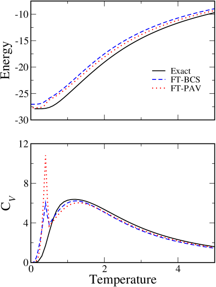
Figure 1: Evolution of the energy (Top) and heat capacity (Bottom) obtained with the FT-BCS (dashed line), PAV (filled circles) and exact solution (thick line) for a system of $N=10$ particles.

As it is well know, in addition to the systematic overestimation of the energy, the FT-BCS theory suffers from the sharp superfluid to normal phase transition as the temperature increases. On opposite, the exact solution display a much smoother behaviour. It is clearly seen in this figure that, except in the very small temperature case, the FT-BCS+PAV does even a worse job and does not cure the threshold effect.

Extrapolating the improvement generally observed at $T=0$ Hup11 to the finite temperature case, one can anticipate a much better description if VAP is performed. In that case, the variational principle (2) should be minimized by both varying the components $(u_{k},v_{k})$ and the energy $E_{k}$ consistently Ese93 . While in principle possible, such minimization has never been performed due to the fact that the hamiltonian $\hat{h}$ and the operator ${\hat{P}}_{N}\exp(-\beta\hat{h}){\hat{P}}_{N}$ do not commute and therefore cannot be diagonalized simultaneously. As a consequence, while a guideline of practical implementation has been proposed long ago in Ese93 , except in the case of the two-level degenerate system, the predictive power of VAP at finite temperature (called hereafter FT-VAP) has never been attested.

In the present work, we applied the FT-VAP following the strategy proposed in ref. Ese93 . In practice, the variational principle is minimized by writing first the energy in terms of the one- and two-body density of the projected density, both of them written as a non-trivial function of the $u_{k}$, $v_{k}$ and $E_{k}$ (see Eq. (36) in ref. Ese93 ). The minimization is carried out via a sequential quadratic programming method by using the $v_{k}$ and $E_{k}$ as variational parameters. To compute the free energy without approximation, at each iteration of the minimization, the entropy is calculated by

$$S=-k_{B}\sum_{i}D^{N}_{i}logD^{N}_{i}$$ (6)

where $D^{N}_{i}$ are the eigenvalues of the statistical operator $\exp(-\beta\hat{h})/Z$ in the Fock space composed by all the many-body configurations with $N$ particles. Each configuration is characterized by $\eta$ pairs and $I$ unpaired particles, with 2$\eta+I=N$. Moreover, since states with a different number of unpaired particles cannot be connected by the operator $\exp(-\beta\hat{h})$, the problem is reduced to the diagonalization of block matrices for each allowed seniority I. The required computational cost is thus given essentially by two operations, i.e. the calculation of the matrix elements of the statistical operators and the diagonalization itself. For the latter, a standard QR algorithm is used. The calculation of the matrix elements is done by using the bit representation of the many-body states (see for example ref. Caurier ). Each configuration is identified by an integer word whose bits correspond to the single particle levels and have value 1 or 0 depending on whether the level is occupied or empty. In such a way all the matrix elements can be obtained by using very simple logical operations which allow to perform calculations much faster.

In figure 2, the result obtained in FT-VAP is compared to the exact solution for a system of $N=10$ particles at various temperature. In FT-VAP, the gap is given by Eq. (42) of ref. Ese93 while in the exact case it is computed through:

$$\Delta=\sqrt{-G(E-E_{0}})$$ (7)

where $E$ is the total exact energy and $E_{0}$ is given by

$$E_{0}=\sum_{i}\left(\varepsilon_{i}-\frac{G}{2}n_{i}\right)n_{i}$$ (8)

containing both the single-particle and the self-energy terms, $n_{i}$ being the occupation numbers. In this figure, we see that, except for the small systematic difference observed for the gap, the FT-VAP approach provides a perfect description of the thermodynamics of a system with fixed particle number in any range of temperature. None of the limitations Ros97 ; Din08 appearing in other mean-field based theories are seen. In particular, the entropy, that is an approximation in FT-VAP, perfectly matches the exact one. The same quality of agreement is found also at higher temperature (up to T= 10).

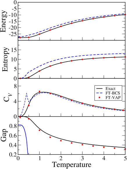
Figure 2: Illustration of the predictive power of the FT-VAP. From top to bottom, the energy $\langle H\rangle$, the entropy, the heat capacity and the average gap obtained with the FT-VAP (filled circles) are compared to the exact (thick line) and FT-BCS case (dashed line) for a system of $N=10$ particles.

We further investigated the applicability of FT-VAP for odd number of particles. Taking advantage of the fact that the FT-BCS density mixes up odd and even parities as soon as a non-zero temperature is applied, we used the same technique as in the even case. The only difference is that now the projector entering in the density (Eq. (1)) corresponds to an odd number of particles. In top panel of figure 3, the pairing gap obtained in FT-VAP for $N=10$ and $N=11$ particles is compared to the exact case. In bottom panel of this figure, the spin susceptibility $\chi$ defined as Dil00

$$\chi(T) = -T\left.\frac{\partial^{2}\ln{Z}}{\partial B^{2}}\right|_{B=0},$$ (9)

is shown for the two cases.

In the limit of small magnetic field, the susceptibility identifies with the fluctuation of the magnetization $\hat{M}=-\mu_{B}\sum_{\sigma,i}\sigma\hat{c}^{\dagger}_{i,\sigma}\hat{c}_{i,\sigma}$ Van06 , i.e.

$$\chi(T) = -\frac{1}{T}\left(\langle\hat{M}^{2}\rangle-\langle\hat{M}\rangle^{2}\right).$$ (10)

In small systems, large differences are observed in the thermodynamics of odd and even systems Von01 . This is clearly seen especially at low temperature for the gap. The spin susceptibility further underlines the differences. The FT-VAP perfectly grasps the thermodynamics of odd systems and one cannot distinguish its result from the exact solution.

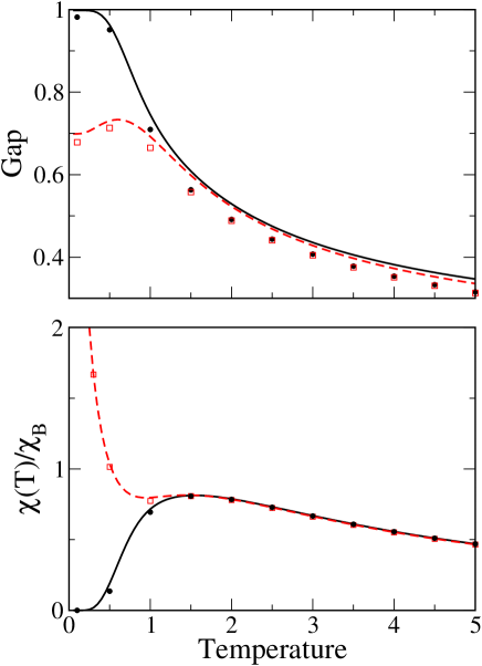
Figure 3: Evolution of the mean gap (upper panel ) and spin susceptibility (lower panel) for $N=10$ (filled circles) and $N=11$ (open squares) particles as a function of $T$ obtained with the FT-VAP. The corresponding exact result for the even and odd systems are presented respectively with solid and dashed lines. In this figure, the spin susceptibility is normalized by the bulk high temperature value $\chi_{B}=2\mu^{2}_{B}/\Delta\varepsilon$.

In the present letter, we applied for the first time the variation after projection approach to describe the canonical properties of a superconducting system. The minimization of the free energy is made with no approximation on the entropy. The FT-VAP provides a perfect reproduction of the exact result in the Richardson Hamiltonian case both in the low and high temperature limit and does not have the limitation of other mean-field based approaches. Due to the necessity to make use of explicit diagonalization for the entropy, the present approach is still restricted to rather small number of particles. Nevertheless, we believe that the result obtained here is sufficiently promising that in the near future, an effort should be made to promote the FT-VAP and make it more versatile. It should be mentioned that the present method provides a natural extension of the FT-BCS or FT-HFB theory presently used to describe nuclei within the Energy Density Functional framework applied at finite temperature edf .

References

- (1) F. Braun and J. von Delft, Phys. Rev. Lett. 81, 4712 (1998).
- (2) J. von Delft and D. C. Ralf, Phys. Rep. 345, 61 (2001).
- (3) F. Braun and J. von Delft, Phys. Rev. B 99, 9527 (1999).
- (4) R. Balian, H.Flocard, M. Vénéroni, arXiv:cond-mat/9802006.
- (5) A. Di Lorenzo, R. Fazio, F. W. J. Hekking, G. Falci, A. Mastellone, and G. Giaquinta Phys. Rev. Lett. 84, 550 (2000).
- (6) P. Ring and P. Schuck, The Nuclear Many-Body Problem, Springer-Verlag, Berlin, (1980).
- (7) M. Bender, P.-H. Heenen, and P.-G. Reinhard, Rev. Mod. Phys. 75, 121 (2003).
- (8) M.A. Fernández and J.L. Egido, Phys. Scr. T125, 87 (2006).
- (9) G. Hupin and D. Lacroix, Phys. Rev. C 83, 024317 (2011).
- (10) C. Esebbag and J. L. Egido, Nucl. Phys. A 552, 205 (1993).
- (11) R. Balian, H. Flocard and M. Vénéroni, Phys. Rep. 317, 251 (1999).
- (12) R. Rossignoli and P. Ring, Ann. Phys. (NY) 235, 350 (1994).
- (13) K. Tanabe and H. Nakada Phys. Rev. C 71, 024314 (2005).
- (14) N. Dinh Dang and A. Arima Phys. Rev. C 68, 014318 (2003).
- (15) N. Dinh Dang and N. Quang Hung Phys. Rev. C 77, 064315 (2008), and references therein.
- (16) V. Yu. Ponomarev and A. I. Vdovin Phys. Rev. C 72, 034309 (2005).
- (17) R. Rossignoli and N. Casona, Phys. Lett. B 394, 242 (1997); R. Rossignoli, N. Casona and J.L. Egido, Nucl. Phys. A 605, 1 (1996).
- (18) J. von Delft, A.D. Zaikin, D. S. Golubrv and W. Tichy, Phys. Rev. Lett. 77, 3189 (1996).
- (19) R. W. Richardson and N. Sherman, Nucl. Phys. 52, 221 (1964); R. W. Richardson, Phys. Rev. 141, 949 (1966); J. Math. Phys. 9, 1327 (1968).
- (20) A. Volya, B. A. Brown and Z.Zelevinsky, Phys. Lett. B 509, 37 (2001); T. Sumaryada and Alexander Volya Phys. Rev. C 76, 024319 (2007).
- (21) K. Van Houcke, S. M. A. Rombouts, and L. Pollet Phys. Rev. E 73, 056703 (2006).
- (22) E. Caurier, G. Martínez-Pinedo, F. Nowacki, A. Poves and A. P. Zuker, Rev. Mod. Phys. 77, 427 (2005).
- (23) V. Martin, J.L. Egido and L.M. Robledo, Phys. Rev. C 68, 034327 (2003); E. Khan, N. Van Gian qnd N. Sandulescu, Nuclear Physics A 789, 94 (2007); A. F. Fantina, J. Margueron, P. Donati and P.M. Pizzochero, J. Phys. G: Nucl. and Part. Phys. 38, 025101 (2001).