$B\to K\eta^{(\prime)}\gamma$ decays in the standard model
and in scenarios with universal extra dimensions

Abstract

We study the radiative $B\to K\eta^{(\prime)}\gamma$ decays, which are important to investigate CP violation, and are also relevant to assess the role of the exclusive modes induced by the $b\to s\gamma$ transition to saturate the inclusive $B\to X_{s}\gamma$ decay rate. Moreover, these channels do not display the same hierarchy as $B\to K\eta^{(\prime)}$ modes, for which the decay into $\eta^{\prime}$ is enhanced with respect to one into $\eta$. The three-body radiative decays reverse the role: we find that this experimentally observed behavior (although affected by a large uncertainty in the case of the $\eta^{\prime}$) is reproduced in the theoretical analysis. We compute a $B^{*}\to K$ form factor, needed for this study, using light cone QCD sum rules, and discuss a relation expected to hold in the large energy limit for the light meson. Finally, we examine $B\to K\eta\gamma$ in two extensions of the standard model with universal extra dimensions, to investigate the sensitivity of this rare mode to such a kind of new physics effects.

I Introduction

The decay processes driven by the flavor changing neutral current (FCNC) $b\to s$ transitions provide efficient tests of the standard model (SM) and can display deviations signaling new physics (NP) phenomena. Among such processes, the $b\to s$ induced decays of $B$ mesons are the best studied and experimentally investigated; several of them have been observed through dedicated experimental analyses which have produced measurements of a variety of observables useful, on the basis of information on both inclusive and exclusive channels, to confirm the SM and constrain NP scenarios Buchalla:2008jp .

The radiative $b\to s\gamma$ transition, on which we focus here, is particularly relevant. Branching fractions have been measured for the inclusive $B\to X_{s}\gamma$ mode, as well as for several exclusive channels, namely $B\to K^{*}(892)\gamma$, $B\to K_{1}(1270)\gamma$, $B\to K^{*}_{2}(1430)\gamma$, $B\to K\eta\gamma$, $B\to K\eta^{\prime}\gamma$, $B\to K\phi\gamma$, $B\to K^{*}(892)\pi\gamma$ and $B\to K\pi\pi\gamma$, both for neutral and charged $B$ mesons pdg . The observed exclusive modes do not saturate the inclusive rate, therefore the scrutiny of the exclusive transitions is mandatory in view of understanding the hadronization process for this class of channels. This is one of the motivations of the present analysis of the three-body $B\to K\eta^{(\prime)}\gamma$ modes. Moreover, there are other features making the multibody decays induced by $b\to s\gamma$ interesting to be studied. First, the time-dependent CP asymmetry in the neutral modes $B^{0}\to K^{0}_{S,L}\eta^{(\prime)}\gamma$ is sensitive to NP, which may also manifest itself in producing right-handed photons; indeed, in the SM the photons produced in the $b\to s\gamma$ transition are mainly left-handed, the amplitude for emitting right-handed photons being suppressed by the quark mass ratio $m_{s}/m_{b}$ hep-ph/0410036 . Furthermore, the branching fractions of $B\to K\eta\gamma$ and $B\to K\eta^{\prime}\gamma$ do not obey the same hierarchy as in the two-body decays $B\to K\eta$ and $B\to K\eta^{\prime}$, the last process being enhanced with respect to the former one. The enhancement of two-body hadronic transitions with $\eta^{\prime}$ in the final state is common to several $B$ and $D$ decays, and is not yet fully understood. In the case of $D_{s}\to\eta^{(\prime)}\pi\,,\,\,\eta^{(\prime)}\rho$, the gluon content of the $\eta^{\prime}$ has been indicated as playing an important role Colangelo:2001cv . For $B\to K\eta$ and $B\to K\eta^{\prime}$, a possible explanation of the hierarchy between the two decay rates has been found in the destructive interference among the penguins contributions Lipkin:1990us , and, modulo large uncertainties, this has been numerically reproduced in the framework of QCD factorization Beneke:2002jn . On the contrary, the radiative modes $B\to K\eta\gamma$ and $B\to K\eta^{\prime}\gamma$ show the opposite trend, as one can infer from the results provided by Belle Nishida:2004fk ; arXiv:0810.0804 and BaBar collaborations Aubert:2006vs ; Aubert:2008js , and collected in Table 1: such an outcome deserves investigations.

Table 1: Experimental results for the $B\to K\eta^{(\prime)}\gamma$ branching fractions ($\times 10^{6}$) from Belle and BaBar. The upper limits are at $90\%$ CL.

Mode	Belle collaboration	BaBar collaboration
$B^{+}\to K^{+}\,\eta\,\gamma$	$8.4\pm 1.5\pm^{1.2}_{0.9}$      Nishida:2004fk	$7.7\pm 1.0\pm 0.4$         Aubert:2008js
$B^{0}\to K^{0}\,\eta\,\gamma$	$8.7\pm^{3.1}_{2.7}\pm^{1.9}_{2.6}$       Nishida:2004fk	$7.1\pm^{2.1}_{2.0}\pm 0.4$            Aubert:2008js
$B^{+}\to K^{+}\,\eta^{\prime}\,\gamma$	$3.6\pm 1.2\pm 0.4$   arXiv:0810.0804	$1.9\pm^{1.5}_{1.2}\pm 0.1$    ($<4.2$) Aubert:2006vs
$B^{0}\to K^{0}\,\eta^{\prime}\,\gamma$	$<6.4$        arXiv:0810.0804	$1.1\pm^{2.8}_{2.0}\pm 0.1$    ($<6.6$) Aubert:2006vs

From the experimental side, the BaBar collaboration has also measured the mixing induced ($S$) and direct ($C$) CP asymmetries in the $B^{0}\to K_{S}^{0}\eta\gamma$ transition. At present they are both compatible with zero: $\displaystyle S=-0.18\pm^{0.49}_{0.46}\pm 0.12$ and $\displaystyle C=-0.32\pm^{0.40}_{0.39}\pm 0.07$ Aubert:2008js .

The processes $B\to K\eta^{(\prime)}\gamma$ have been studied in Ref.Fajfer:2008zy considering exclusively the regions of the phase space where one of the two pseudoscalar mesons in the final state is soft, while the photon is hard. Describing the amplitudes as taking contributions only from virtual intermediate $B^{*}$ and $B_{s}^{*}$, the Heavy Quark Effective Theory together with the light meson chiral perturbation theory ($\chi$HQET) has been employed to describe the decays in corners of the Dalitz plot; moreover, the $\eta-\eta^{\prime}$ mixing has been described in the octet-singlet mixing scheme. As a result, a fraction of about $10\%$ of the measured $B\to K\eta\gamma$ branching ratio has been obtained.

In the present study we improve the analysis in many respects. We take into account several possible underlying transitions, depicted in Fig. 1, observing that, in addition to $b\to s\gamma$, the transition $b\to s\bar{q}q$ can contribute to the processes. In particular, the explicit calculation shows that the diagram (1) with intermediate virtual $K^{*}$ is important, together with diagrams (3) and (4), while the one with intermediate $K^{*}_{2}(1430)$ and the other diagrams in Fig. 1 are smaller. Furthermore, we do not confine ourselves to portions of the phase space, but we extend the study to the full three-body Dalitz plot. This requires new information, namely the $B^{*}\to K$ and $B_{s}^{*}\to\eta$ form factors, which we compute by light cone QCD sum rules for a physical value of the beauty quark mass and for a wide range of four-momentum transferred. Finally, we consider the $\eta-\eta^{\prime}$ system in the flavor basis, in which the mixing is described by a single mixing angle experimentally determined with high accuracy by the KLOE collaboration from radiative $\phi\to\eta^{(\prime)}\gamma$ decay data. In this way, results for the SM can be obtained, and the effects of NP extensions, such as scenarios with universal extra dimensions (UED), can be examined.

All these topics are described in the forthcoming sections. In particular, in Section II we set up the stage of our calculation, considering the diagrams taken into account in the theoretical description of $B\to K\eta^{(\prime)}\gamma$. We provide the expressions of the various amplitudes and identify the quantities necessary for their evaluation. Section III is devoted to the light cone QCD sum rule determination of the form factor $T_{1}^{B^{*}\to K}$, which enters in the analysis of $B\to K\eta^{(\prime)}\gamma$ transitions; we collect in the Appendix the definitions of the needed kaon light-cone distribution amplitudes (LCDA). The computation of the decay rates is carried out in Sec.IV in the SM; the sensitivity to NP effects of one and two universal extra dimension scenarios is also investigated. Section V contains our conclusions.

II The decays $B\to K\eta^{(\prime)}\gamma$

We consider the transitions ${\overline{B}^{0}}(p)\to{\overline{K}^{0}}(p_{K})\,\eta^{(\prime)}(p_{\eta^{(\prime)}})\,\gamma(q,\epsilon)$, where $p$, $p_{K}$ and $p_{\eta^{(\prime)}}$ are the four momenta of $B$, $K$ and $\eta^{(\prime)}$, respectively, while $q$ and $\epsilon$ are the photon four momentum and polarization vector. Although we refer to the decays of the neutral ${\overline{B}^{0}}$, in the following we omit the charge adopting a simpler notation; at the end of our study we shall comment on the charged $B$ meson decays. The three-body transitions can be described as proceeding through intermediate states: The ones that we take into account are displayed in Fig. 1. The first two diagrams (1) and (2) take contribution from intermediate $K^{*}(892)$ and $K_{2}^{*}(1430)$, respectively, which have width: $\Gamma(K^{*0}(892))=48.7\pm 0.8$ MeV and $\Gamma(K^{*}_{2}(1430))=98.5\pm 2.9$ MeV pdg . Higher kaon excitations are expected to give a smaller contribution, due to their larger widths and to the suppression provided by their propagators in the corresponding diagrams.

Figure 1: Some diagrams contributing to the decays ${\overline{B}^{0}}\to{\overline{K}^{0}}\eta^{(\prime)}\gamma$. The dots indicate em and strong couplings; the squares indicate weak vertices.

The two diagrams (3) and (4) have $B^{*}$ or $B_{s}^{*}$ as intermediate states, which are very narrow so that we neglect their widths. The diagram (5) takes contribution from the intermediate $\phi(1020)$ decaying to $\eta^{(\prime)}\gamma$ and having $\Gamma(\phi(1020))=4.26\pm 0.04$ MeV; $B^{*}$ is the intermediate state also in the last diagram, which involves the radiative $B^{*}B\gamma$ vertex.

To calculate the amplitudes corresponding to the diagrams in Fig. 1 we need the effective weak Hamiltonian describing the $b\to s\gamma$ and $b\to s\,{\rm gluon}$ transition. In the SM this reads Buchalla:1995vs :

$$H_{eff}=-{G_{F}\over\sqrt{2}}V_{tb}V_{ts}^{*}\left(\sum_{i=1}^{6}C_{i}\,O_{i}+C_{7\gamma}\,O_{7\gamma}+C_{8G}\,O_{8G}\right)\,.$$ (1)

$G_{F}$ is the Fermi constant and $V_{ij}$ are elements of the Cabibbo-Kobayashi-Maskawa mixing matrix; we neglect terms proportional to $V_{ub}V_{us}^{*}$ since the ratio $\displaystyle\left|{V_{ub}V_{us}^{*}\over V_{tb}V_{ts}^{*}}\right|$ is of ${O}(10^{-2})$. $C_{i}$ are Wilson coefficients, while $O_{i}$ are local operators written in terms of quark and gluon fields:

$$O_{1} = ({\bar{s}}_{L\alpha}\gamma^{\mu}b_{L\alpha})({\bar{c}}_{L\beta}\gamma_{\mu}c_{L\beta})$$

$$O_{2} = ({\bar{s}}_{L\alpha}\gamma^{\mu}b_{L\beta})({\bar{c}}_{L\beta}\gamma_{\mu}c_{L\alpha})$$

$$O_{3} = ({\bar{s}}_{L\alpha}\gamma^{\mu}b_{L\alpha})[({\bar{u}}_{L\beta}\gamma_{\mu}u_{L\beta})+...+({\bar{b}}_{L\beta}\gamma_{\mu}b_{L\beta})]$$

$$O_{4} = ({\bar{s}}_{L\alpha}\gamma^{\mu}b_{L\beta})[({\bar{u}}_{L\beta}\gamma_{\mu}u_{L\alpha})+...+({\bar{b}}_{L\beta}\gamma_{\mu}b_{L\alpha})]$$

$$O_{5} = ({\bar{s}}_{L\alpha}\gamma^{\mu}b_{L\alpha})[({\bar{u}}_{R\beta}\gamma_{\mu}u_{R\beta})+...+({\bar{b}}_{R\beta}\gamma_{\mu}b_{R\beta})]$$ (2)

$$O_{6} = ({\bar{s}}_{L\alpha}\gamma^{\mu}b_{L\beta})[({\bar{u}}_{R\beta}\gamma_{\mu}u_{R\alpha})+...+({\bar{b}}_{R\beta}\gamma_{\mu}b_{R\alpha})]$$

$$O_{7\gamma} = {e\over 16\pi^{2}}\left[m_{b}({\bar{s}}_{L\alpha}\sigma^{\mu\nu}b_{R\alpha})+m_{s}({\bar{s}}_{R\alpha}\sigma^{\mu\nu}b_{L\alpha})\right]F_{\mu\nu}$$

$$O_{8G} = {g_{s}\over 16\pi^{2}}m_{b}\Big{[}{\bar{s}}_{L\alpha}\sigma^{\mu\nu}\Big{(}{\lambda^{a}\over 2}\Big{)}_{\alpha\beta}b_{R\beta}\Big{]}\;G^{a}_{\mu\nu}\,\,.$$

$\alpha$, $\beta$ are color indices, $\displaystyle b_{R,L}={1\pm\gamma_{5}\over 2}b$, and $\displaystyle\sigma^{\mu\nu}={i\over 2}[\gamma^{\mu},\gamma^{\nu}]$; $e$ and $g_{s}$ are the electromagnetic and the strong coupling constant, respectively, $m_{b}$ and $m_{s}$ are the beauty and the strange quark masses, while $F_{\mu\nu}$ in $O_{7\gamma}$ and $G^{a}_{\mu\nu}$ in $O_{8\gamma}$ denote the electromagnetic and the gluonic field strength tensors. $\lambda^{a}$ are the Gell-Mann matrices.

The Wilson coefficients appearing in (1) have been computed at next-to-next-to-leading order in the standard model nnlo . The most relevant contribution to $b\to s\gamma$ comes from the operator $O_{7\gamma}$, which is a magnetic penguin specific of such a transition and originates from the mass insertion on the external $b$-quark line in the QED penguin. The term proportional to $m_{s}$ contributes much less than the one proportional to $m_{b}$, and this is the reason for which the emission of left-handed photons dominates over that of right-handed ones in the SM. Since the coefficient $C_{7\gamma}$ depends on the regularization scheme, it is convenient to consider at leading order a combination that is regularization scheme independent Buras:1993xp :

$$C_{7\gamma}^{(0)eff}(\mu_{b})=\eta^{16\over 23}C_{7\gamma}^{(0)}(\mu_{W})+{8\over 3}\left(\eta^{14\over 23}-\eta^{16\over 23}\right)C_{8G}^{(0)}(\mu_{W})+C_{2}^{(0)}(\mu_{W})\sum_{i=1}^{8}h_{i}\eta^{a_{i}}\,\,\,,$$ (3)

where $\displaystyle\eta={\alpha_{s}(\mu_{W})\over\alpha_{s}(\mu_{b})}$ and $C_{2}^{(0)}(\mu_{W})=1$ (the superscript $(0)$ stays for leading log approximation); furthermore,

$$a_{1}={14\over 23}\hskip 11.38092pta_{2}={16\over 23}\hskip 11.38092pt a_{3}={6\over 23}\hskip 11.38092pta_{4}=-{12\over 23}$$

$$a_{5}=0.4086\hskip 11.38092pta_{6}=-0.4230\hskip 11.38092pt a_{7}=-0.8994\hskip 11.38092pta_{8}=0.1456$$

$$h_{1}=2.2996\hskip 11.38092pth_{2}=-1.0880\hskip 11.38092pt h_{3}=-{3\over 7}\hskip 11.38092pth_{4}=-{1\over 14}$$ (4)

$$h_{5}=-0.6494\hskip 11.38092pth_{6}=-0.0380\hskip 11.38092pt h_{7}=-0.0185\hskip 11.38092pth_{8}=-0.0057\,\,\,.$$

The effective weak vertex $O_{7\gamma}$ contributes to the diagrams (1-4) in Fig. 1 through hadronic matrix elements that we define below. However, before doing that, we turn to the $\eta-\eta^{\prime}$ system.

The $\eta-\eta^{\prime}$ mixing is usually described in two different schemes, adopting either the singlet-octet or the quark flavor (QF) basis, and in each scheme two mixing angles are involved Feldmann:1999uf . Here we adopt the quark flavor basis defining

$$\left|\eta_{q}\right\rangle = {1\over\sqrt{2}}\left(\left|{\bar{u}}u\right\rangle+\left|{\bar{d}}d\right\rangle\right)$$

$$\left|\eta_{s}\right\rangle = \left|{\bar{s}}s\right\rangle\,\,,$$ (5)

so that the $\eta$-$\eta^{\prime}$ system can be described in terms of the mixing angles $\varphi_{q}$ and $\varphi_{s}$:

$$\left|\eta\right\rangle = \cos\,\varphi_{q}\left|\eta_{q}\right\rangle-{\sin}\,\varphi_{s}\left|\eta_{s}\right\rangle$$

$$\left|\eta^{\prime}\right\rangle = {\sin}\,\varphi_{q}\left|\eta_{q}\right\rangle+{\cos}\,\varphi_{s}\left|\eta_{s}\right\rangle\,\,\,\,.$$ (6)

The difference between $\varphi_{q}$ and $\varphi_{s}$ is due to OZI-violating effects and is experimentally found to be small ($\varphi_{q}-\varphi_{s}<5^{\circ}$), so that it has been proposed that the approximation of describing the $\eta-\eta^{\prime}$ mixing in the QF basis and a single mixing angle is suitable Feldmann:1999uf . The simplification $\varphi_{q}\simeq\varphi_{s}\simeq\varphi$ is supported by a QCD sum rule analysis of the $\phi\to\eta\gamma$ and $\phi\to\eta^{\prime}\gamma$ decays DeFazio:2000my . A precise determination of the $\eta-\eta^{\prime}$ mixing angle has been obtained by the KLOE Collaboration measuring the ratio $\displaystyle{\Gamma(\phi\to\eta^{\prime}\gamma)\over\Gamma(\phi\to\eta\gamma)}$ in the flavor basis with a single mixing angle, with the result: $\varphi=\big{(}41.5\pm 0.3_{stat}\pm 0.7_{syst}\pm 0.6_{th}\big{)}^{\circ}$ kloe . This analysis has been improved performing a global fit of the transitions $V\to P\gamma$ and $P\to V\gamma$ ($V=\phi,\,\omega,\,\rho$ and $P=\pi^{0},\,\eta,\,\eta^{\prime}$), allowing a gluonium content in the $\eta^{\prime}$ and including the measurement of the ratio $\displaystyle{\Gamma(\eta^{\prime}\to\gamma\gamma)\over\Gamma(\pi^{0}\to\gamma\gamma)}$ Ambrosino:2009sc . The outcome is that, even though the gluonium content of the $\eta^{\prime}$ is significant, the result for the $\eta-\eta^{\prime}$ mixing angle is only negligibly affected. Therefore, we set $\varphi$ to the value quoted above.

Let us now consider in turn the various diagrams in Fig. 1.

• Diagrams 1 and 2

The corresponding amplitudes read:

$$A_{1} = A(B\to K^{*}\gamma){i\over s-m_{K^{*}}^{2}+i\,m_{K^{*}}\,\Gamma_{K^{*}}}A(K^{*}\to K\eta^{(\prime)})$$ (7)

$$A_{2} = A(B\to K^{*}_{2}\gamma){i\over s-m_{K^{*}_{2}}^{2}+i\,m_{K^{*}_{2}}\,\Gamma_{K^{*}_{2}}}A(K^{*}_{2}\to K\eta^{(\prime)})\,\,,$$ (8)

with

$$A(B\to K^{*}_{(2)}\gamma)=C\epsilon^{*\mu}\left[(m_{b}+m_{s})<K^{*}_{(2)}(p_{K},{\tilde{\epsilon}})|{\bar{s}}\sigma_{\mu\nu}q^{\nu}b|B(p)>+(m_{b}-m_{s})<K^{*}_{(2)}(p_{K},{\tilde{\epsilon}})|{\bar{s}}\sigma_{\mu\nu}q^{\nu}\gamma_{5}b|B(p)>\right]\,\,\,,$$

to be computed for an on-shell ($q^{2}=0$) photon, defining $s=(p-q)^{2}=M^{2}_{K\eta^{(\prime)}}$. The factor $C$ is $C=4\displaystyle{G_{F}\over\sqrt{2}}V_{tb}V_{ts}^{*}C_{7}^{(eff)}\displaystyle{e\over 16\pi^{2}}$. The hadronic matrix elements of weak Hamiltonian operators are parametrized in terms of form factors:

$$<K^{*}_{(2)}(p_{K},{\tilde{\epsilon}})|{\bar{s}}\sigma_{\mu\nu}q^{\nu}b|B(p)> = i\epsilon_{\mu\nu\alpha\beta}{\tilde{\epsilon}}^{*\nu}p^{\alpha}p^{\beta}_{K}\;2\;T_{1}^{B\to K^{*}_{(2)}}(q^{2})$$ (9)

$$<K^{*}_{(2)}(p_{K},{\tilde{\epsilon}})|{\bar{s}}\sigma_{\mu\nu}q^{\nu}\gamma_{5}b|B(p)> = \Big{[}{\tilde{\epsilon}}^{*}_{\mu}(M_{B}^{2}-s)-({\tilde{\epsilon}}^{*}\cdot q)(p+p_{K})_{\mu}\Big{]}\;T_{2}^{B\to K^{*}_{(2)}}(q^{2})$$ (10)

$$+ ({\tilde{\epsilon}}^{*}\cdot q)\left[q_{\mu}-{q^{2}\over M_{B}^{2}-s}(p+p_{K})_{\mu}\right]\;T_{3}^{B\to K^{*}_{(2)}}(q^{2})\;\,\,\,,$$

with ${\tilde{\epsilon}}$ denoting the polarization vector of the $K^{*}_{(2)}$ mesons; in the case of $K^{*}_{2}(1430)$, which is a spin 2 particle, the polarization is described by a two indices symmetric and traceless tensor, therefore in (9-10) it is understood that ${\tilde{\epsilon}}^{\alpha}={\tilde{\epsilon}}^{\alpha\beta}\displaystyle{p_{\beta}\over M_{B}}$. The condition holds: $T_{1}^{B\to K^{*}_{(2)}}(0)=T_{2}^{B\to K^{*}_{(2)}}(0)$. The variable $s$ in the definition of the hadronic matrix elements takes into account that the $K^{*}_{(2)}$ mesons are off-shell, and is needed to ensure gauge invariant amplitudes.

In the same diagrams strong vertices also appear, which are defined as follows:

$$A(K^{*}\to K\eta^{(\prime)}) = g_{K^{*}K\eta^{(\prime)}}\,{\tilde{\epsilon}}\cdot p_{\eta^{(\prime)}}$$ (11)

$$A(K^{*}_{2}\to K\eta^{(\prime)}) = g_{K^{*}_{2}K\eta^{(\prime)}}\,{\tilde{\epsilon}}^{\alpha\beta}p_{\eta^{(\prime)}\alpha}\,p_{\eta^{(\prime)}\beta}\,\,.$$ (12)

Within the flavor scheme for the $\eta-\eta^{\prime}$ mixing the relations $g_{K^{*}K\eta}=(\cos\varphi+\sqrt{2}\sin\varphi)g_{K^{*+}K^{+}\pi^{0}}$ and $g_{K^{*}K\eta^{\prime}}=(\sin\varphi-\sqrt{2}\cos\varphi)g_{K^{*+}K^{+}\pi^{0}}$ can be worked out. Assuming the width of $K^{*+}$ saturated by the two modes $K^{*+}\to K^{+}\pi^{0},\,K^{0}\pi^{+}$, and using the relation $g_{K^{*+}K^{0}\pi^{+}}=\sqrt{2}\,g_{K^{*+}K^{+}\pi^{0}}$, from $\Gamma(K^{*+})=50.8\pm 0.9$ MeV we obtain $g_{K^{*+}K^{+}\pi^{0}}=6.5\pm 0.06$.

The strong coupling $g_{K^{*}_{2}K\eta}$ can be estimated, although with a large uncertainty, using the measurement ${\cal B}(K^{*}_{2}\to K\eta)=(1.5\pm^{3.4}_{1.0})\times 10^{-3}$ pdg together with $\Gamma(K^{*}_{2})$, obtaining: $g_{K^{*}_{2}K\eta}=1.43\pm 1.60$ GeV^-1. On the other hand, no information is available for $g_{K^{*}_{2}K\eta^{\prime}}$; however, since, as we shall see, the contribution of this diagram is small in the case of $\eta$, it is reasonable to neglect it also in the case of the $\eta^{\prime}$ in the final state.

• Diagrams 3 and 4

The two amplitudes read:

$$A_{3} = A(B\to B^{*}\eta^{(\prime)}){i\over t-m_{B^{*}}^{2}}A(B^{*}\to K\gamma)$$ (13)

$$A_{4} = A(B\to B^{*}_{s}K){i\over u-m_{B^{*}_{s}}^{2}}A(B^{*}_{s}\to\eta^{(\prime)}\gamma)\,\,,$$ (14)

with

$$A(B^{*}\to K\gamma) = C\epsilon^{*\nu}\left[(m_{b}+m_{s})<K(p_{K})|{\bar{s}}\sigma_{\mu\nu}q^{\nu}b|B^{*}(p^{\prime},{\tilde{\epsilon}})>+(m_{b}-m_{s})<K(p_{K})|{\bar{s}}\sigma_{\mu\nu}q^{\nu}\gamma_{5}b|B^{*}(p^{\prime},{\tilde{\epsilon}})>\right]\,\,\,,$$

$$A(B^{*}_{s}\to\eta^{(\prime)}\gamma) = C\epsilon^{*\nu}\left[(m_{b}+m_{s})<\eta^{(\prime)}(p_{\eta^{(\prime)}})|{\bar{s}}\sigma_{\mu\nu}q^{\nu}b|B^{*}_{s}(p^{\prime},{\tilde{\epsilon}})>+(m_{b}-m_{s})<\eta^{(\prime)}(p_{\eta^{(\prime)}})|{\bar{s}}\sigma_{\mu\nu}q^{\nu}\gamma_{5}b|B^{*}_{s}(p^{\prime},{\tilde{\epsilon}})>\right],$$

and

$$<K(p_{K})|{\bar{s}}\sigma_{\mu\nu}q^{\mu}b|B^{*}(p^{\prime},{\tilde{\epsilon}})> = i\epsilon_{\nu\tau\alpha\beta}{\tilde{\epsilon}}^{\tau}p^{\prime\alpha}p^{\beta}_{K}\;2\;T_{1}^{B^{*}\to K}(q^{2})$$ (15)

$$<K(p_{K})|{\bar{s}}\sigma_{\mu\nu}q^{\mu}\gamma_{5}b|B^{*}(p^{\prime},{\tilde{\epsilon}})> = \Big{[}{\tilde{\epsilon}}_{\nu}(t-m_{K}^{2})-({\tilde{\epsilon}}\cdot q)(p^{\prime}+p_{K})_{\nu}\Big{]}\;T_{2}^{B^{*}\to K}(q^{2})$$ (16)

$$+ ({\tilde{\epsilon}}\cdot q)\left[q_{\nu}-{q^{2}\over t-m_{K}^{2}}(p^{\prime}+p_{K})_{\nu}\right]\;T_{3}^{B^{*}\to K}(q^{2})\;,$$

$$<\eta^{(\prime)}(p_{\eta^{(\prime)}})|{\bar{s}}\sigma_{\mu\nu}q^{\mu}b|B^{*}_{s}(p^{\prime},{\tilde{\epsilon}})> = i\epsilon_{\nu\tau\alpha\beta}{\tilde{\epsilon}}^{\tau}p^{\prime\alpha}p^{\beta}_{\eta^{(\prime)}}\;2\;T_{1}^{B^{*}_{s}\to\eta^{(\prime)}}(q^{2})$$ (17)

$$<\eta^{(\prime)}(p_{\eta^{(\prime)}})|{\bar{s}}\sigma_{\mu\nu}q^{\mu}\gamma_{5}b|B^{*}_{s}(p^{\prime},{\tilde{\epsilon}})> = \Big{[}{\tilde{\epsilon}}_{\nu}(u-m_{\eta^{(\prime)}}^{2})-({\tilde{\epsilon}}\cdot q)(p^{\prime}+p_{\eta^{(\prime)}})_{\nu}\Big{]}\;T_{2}^{B^{*}_{s}\to\eta^{(\prime)}}(q^{2})$$ (18)

$$+ ({\tilde{\epsilon}}\cdot q)\left[q_{\nu}-{q^{2}\over u-m_{\eta^{(\prime)}}^{2}}(p^{\prime}+p_{\eta^{(\prime)}})_{\nu}\right]\;T_{3}^{B^{*}_{s}\to\eta^{(\prime)}}(q^{2})\;.$$

($p^{\prime}$, ${\tilde{\epsilon}}$) denote the four momentum and the polarization vector of the $B^{*}_{(s)}$; moreover $T_{1}^{B^{*}\to K}(0)=T_{2}^{B^{*}\to K}(0)$ and the same for $\eta^{(\prime)}$. The variable $t=(q+p_{K})^{2}$ takes into account the off-shellness of the $B^{*}$ in diagram (3), while the variable $u=(p_{\eta^{(\prime)}}+q)^{2}$ accounts for the off-shellness of the $B_{s}^{*}$ in diagram (4); obviously, $s+t+u=M_{B}^{2}+m_{K}^{2}+m_{\eta^{(\prime)}}^{2}$.

As for the strong vertices appearing in the two amplitudes, we define

$$A(B\to B^{*}\eta^{(\prime)}) = g_{B^{*}B\eta^{(\prime)}}\,\,\,{\tilde{\epsilon}}^{*}\cdot p_{\eta^{(\prime)}}$$ (19)

$$A(B\to B^{*}_{s}K) = g_{B^{*}_{s}BK}\,\,\,{\tilde{\epsilon}}^{*}\cdot p_{K}\,\,.$$ (20)

The two couplings $g_{B^{*}B\eta^{(\prime)}}$ and $g_{B^{*}_{s}BK}$ can be obtained, invoking $SU(3)_{F}$ symmetry, from the analogous quantity $g_{B^{*}B\pi}$: $g_{B^{*}B\eta}=\cos\varphi\,g_{B^{*}B\eta_{q}}=\cos\varphi\,\,g_{B^{*}B\pi}$, $g_{B^{*}B\eta\prime}=\sin\varphi\,g_{B^{*}B\eta_{q}}=\sin\varphi\,\,g_{B^{*}B\pi}$ and $g_{B^{*}_{s}BK}=g_{B^{*}B\pi}$. As for $g_{B^{*}B\pi}$, it can be related to a low-energy parameter $g$ that describes the coupling of heavy mesons belonging to the doublet of heavy-light quark states with spin-parity $J^{P}=(0^{-},1^{-})$ to light pseudoscalar states in the framework of the $\chi$HQET rev : $g_{B^{*}B\pi}={2M_{B}\over f_{\pi}}g$. There are several theoretical determinations of $g$ spanning the range $[0.2,\,0.5]$ Colangelo:1995ph . However, $g$ can be extracted from the measured decay width of $D^{*+}\to D^{0}\pi^{+}$ Anastassov:2001cw , obtaining $g=0.59\pm 0.01\pm 0.07$ Colangelo:2002dg . We use this value in our analysis.

• Diagram 5

The contribution of the intermediate $\phi(1020)$ is represented by the amplitude

$$A_{5}=A(B\to K\phi){i\over u-m_{\phi}^{2}+i\,m_{\phi}\,\Gamma_{\phi}}A(\phi\to\eta^{(\prime)}\gamma)\,\,.$$ (21)

Adopting factorization, the first amplitude in (21) can be written as

$$A(B\to K\phi)={G_{F}\over\sqrt{2}}V_{tb}V_{ts}^{*}a_{w}\langle K(p_{K})|{\bar{s}}\gamma_{\mu}(1-\gamma_{5})b|B(p)\rangle\,\langle\phi(p_{\phi},{\tilde{\epsilon}})|{\bar{s}}\gamma_{\mu}s|0\rangle\,\,,$$ (22)

where $a_{w}$ is an effective Wilson coefficient that we set to the value $a_{w}=0.064\pm 0.009$ from the experimental branching fraction ${\cal B}({\overline{B}}^{0}\to{\overline{K}}^{0}\phi)=(8.6\pm^{1.3}_{1.1})\times 10^{-6}$ pdg . Furthermore, we use the parametrizations

$$\langle K(p_{K})|{\bar{s}}\gamma_{\mu}(1-\gamma_{5})b|B(p)\rangle = f_{+}^{B\to K}(q^{2})(p+p_{K})_{\mu}+f_{-}^{B\to K}(q^{2})(p-p_{K})_{\mu}$$

$$\langle\phi(p_{\phi}{\tilde{\epsilon}})|{\bar{s}}\gamma_{\mu}s|0\rangle = f_{\phi}m_{\phi}{\tilde{\epsilon}}^{*}_{\mu}\,\,.$$ (23)

When these two definitions are inserted in (22) only the form factor $f_{+}^{B\to K}$ contributes, and we adopt for it the determination in Ref.Ball:2004ye . The value $f_{\phi}=(0.232\pm 0.002)$ GeV comes from the experimental datum ${\cal B}(\phi\to e^{+}e^{-})=(2.954\pm 0.030)\times 10^{-4}$.

Following Ref.DeFazio:2000my , the amplitudes $A(\phi\to\eta^{(\prime)}\gamma)$ can be written as

$$A(\phi\to\eta^{(\prime)}\gamma)=-{e\over 3}F^{\phi\to\eta^{(\prime)}\gamma}(q^{2})\epsilon_{\nu\alpha\beta\delta}\epsilon^{*\nu}(p_{\phi})^{\alpha}(p_{\eta})^{\beta}{\tilde{\epsilon}}^{\delta}\,\,.$$ (24)

The form factors $F^{\phi\to\eta^{(\prime)}\gamma}(q^{2})$ were determined using QCD sum rules, providing their values at $q^{2}=0$ (multiplied by the strange quark charge in units of $e$): $|g^{\phi\eta\gamma}|=\displaystyle{{1\over 3}F^{\phi\to\eta\gamma}(0)}=(0.66\pm 0.06)$ GeV^-1 and $|g^{\phi\eta^{\prime}\gamma}|=\displaystyle{{1\over 3}F^{\phi\to\eta^{\prime}\gamma}(0)}=(1.0\pm 0.2)$ GeV^-1 DeFazio:2000my , results used in our analysis.

• Diagram 6

It is possible to show that the diagram (6) provides a tiny contribution with respect to the others. Let us discuss this in the case of the $\eta$. The amplitude can be written in terms of $A(B^{*}\to B\gamma)$ and $A(B^{*}\to K\eta)$. In order to understand how large this contribution is, we can invoke naive factorization, writing $A(B^{*}\to K\eta)={G_{F}\over\sqrt{2}}V_{ub}^{*}V_{us}a_{2}^{eff}\langle K|{\bar{s}}\gamma^{\mu}(1-\gamma_{5})|B^{*}\rangle\langle\eta|{\bar{u}}\gamma_{\mu}(1-\gamma_{5})u|0\rangle$, with $a_{2}^{eff}\simeq-0.286$ an effective Wilson coefficient for color suppressed decays. The $\eta$-current-vacuum matrix element involves (in the flavor basis for the $\eta-\eta^{\prime}$ mixing) the constant $f_{\eta}^{q}=f_{q}\cos{\phi}$ with $f_{q}\simeq f_{\pi}$: $\langle\eta|{\bar{u}}\gamma_{\mu}(1-\gamma_{5})u|0\rangle={i\over\sqrt{2}}\,f_{\eta}^{q}\,(p_{\eta})_{\mu}$. On the other hand, the matrix element $\langle{K}|{\bar{s}}\gamma^{\mu}(1-\gamma_{5})|B^{*}\rangle$ can be decomposed in terms of several form factors; however, when contracted with $(p_{\eta})_{\mu}$, only one of such form factors contributes, usually denoted as $A_{0}(m_{\eta}^{2})$, which in the large energy limit of the final light meson coincides with $T_{1}^{B^{*}\to K}$ computed in the next section. The other ingredient is the radiative amplitude $A(B^{*}\to B\gamma)$, which can be written as $A(B^{*}(p^{\prime},{\tilde{\epsilon}})\to B(p)\gamma(q,\epsilon))=e\left(\displaystyle{e_{b}\over\Lambda_{b}}+\displaystyle{e_{q}\over\Lambda_{q}}\right)\,\epsilon_{\alpha\beta\tau\sigma}\,\epsilon^{*\alpha}\,{\tilde{\epsilon}}^{\beta}\,p^{\tau}\,p^{\prime\sigma}$, with $e_{b}$ ($e_{q}$) the $b$ ($q=d$) quark charge in units of $e$. A determination of the mass parameters $\Lambda_{b}$ and $\Lambda_{q}$ can be found in Colangelo:1994jc : $\Lambda_{b}=4.93$ GeV (close to the $b$ quark mass) and $\Lambda_{q}=0.59$ GeV. As a result, the contribution of the diagram (6) to the branching fraction is ${\cal O}(10^{-13})$. Therefore, in the following we neglect this amplitude.

As it emerges from the above discussion, important quantities are the form factors appearing in the diagrams (1)-(4). In the next section we compute $T_{1}^{B^{*}\to K}(q^{2})$ by light cone QCD sum rules Colangelo:2000dp . SU(3)_F symmetry and the QF $\eta-\eta^{\prime}$ mixing scheme allow also to fix: $T_{1}^{B^{*}_{s}\to\eta}(0)=-\sin\varphi\,T_{1}^{B^{*}\to K}(0)$ and $T_{1}^{B^{*}_{s}\to\eta^{\prime}}(0)=\cos\varphi\,T_{1}^{B^{*}\to K}(0)$. As for $T_{1}^{B\to K^{*}}$, several determinations can be found in the literature; we use the light cone QCD sum rule result $T_{1}^{B\to K^{*}}(0)=0.333\pm 0.028$ Ball:2004rg , to be consistent with the determination of $T_{1}^{B^{*}\to K}$. This value is compatible with the one obtained by three-point QCD sum rules based on the short-distance expansion Colangelo:1995jv . Finally, for $T_{1}^{B\to K^{*}_{2}}$ we use $T_{1}^{B\to K^{*}_{2}}(0)=0.17\pm 0.03\pm 0.04$ Wang:2010ni .

There is a remark concerning the relative strong phases among the various amplitudes. While the sign between the amplitudes (3) and (4) can be fixed invoking $\chi$HQET and the flavor symmetry, the relative phase between, e.g., (1) and (3) does not follow from theoretical arguments. Therefore, we consider it as a parameter to be determined empirically from the experimental data. The phases appearing in the other amplitudes do not play a role in the branching ratio due to the small size of such diagrams.

III Form factor $T_{1}^{B^{*}\to K}(q^{2})$ by light cone QCD sum rules

To compute the form factor $T_{1}^{B^{*}\to K}(q^{2})$ by light cone QCD sum rules (LCSR) we consider the two-point correlation function with the external kaon state

$$\Pi_{\mu\nu}(p^{\prime},q)=i\int d^{4}x\,e^{iq\cdot x}\langle K(p^{\prime})|{\rm T}\left\{J_{\mu}(x),V_{\nu}(0)\right\}|0\rangle\,\,\,\,$$ (25)

where $J_{\mu}={\bar{s}}\sigma_{\alpha\mu}q^{\alpha}b$ is the quark current appearing in the matrix element (15). $V_{\nu}={\bar{b}}\gamma_{\nu}q$ is the vector current with the quantum numbers of the $B^{*}$ meson ($q=u,\,d)$, and its matrix element between the vacuum and the $B^{*}$ state is parametrized in terms of the decay constant $f_{B^{*}}$,

$$\langle B^{*}(p^{\prime}+q,{\tilde{\epsilon}})|{\bar{b}}\gamma_{\nu}q|0\rangle=f_{B^{*}}m_{B^{*}}{\tilde{\epsilon}}^{*}_{\nu}\,\,.$$ (26)

The LCSR method consists in expressing the correlation function Eq.(25) both in QCD and in terms of a hadronic representation. $\Pi_{\mu\nu}$ can be decomposed in independent Lorentz structures, one of which can be used to compute $T_{1}^{B^{*}\to K}$:

$$\Pi_{\mu\nu}(p^{\prime},q)=i\,\,\epsilon_{\mu\alpha\tau\nu}q^{\alpha}p^{\prime\tau}\Pi((p^{\prime}+q)^{2},q^{2})+{\rm other\,\,structures}\,\,.$$ (27)

In terms of hadronic states, the correlation function in (25) can be written as

$$\Pi^{\rm HAD}_{\mu\nu}(p^{\prime},q)=\frac{\langle K(p^{\prime})|J_{\mu}|B^{*}(p^{\prime}+q,{\tilde{\epsilon}})\rangle\langle B^{*}(p^{\prime}+q,{\tilde{\epsilon}})|V_{\nu}|0\rangle}{m_{B^{*}}^{2}-(p^{\prime}+q)^{2}}+\sum_{h}\frac{\langle K(p^{\prime})|J_{\mu}|h(p^{\prime}+q)\rangle\langle h(p^{\prime}+q)|V_{\nu}|0\rangle}{m_{h}^{2}-(p^{\prime}+q)^{2}}$$

and consists in the contribution of the $B^{*}$ meson and of the higher resonances and of the continuum of states $h$. The first term in (III) contributes to the invariant function $\Pi((p^{\prime}+q)^{2},q^{2})$, since

$$\frac{\langle K(p^{\prime})|J_{\mu}|B^{*}(p^{\prime}+q,{\tilde{\epsilon}})\rangle\langle B^{*}(p^{\prime}+q,{\tilde{\epsilon}})|V_{\nu}|0\rangle}{m_{B^{*}}^{2}-(p^{\prime}+q)^{2}}=\,i\,\epsilon_{\mu\alpha\tau\nu}q^{\alpha}p^{\prime\tau}\,\,{2\,T_{1}^{B^{*}\to K}(q^{2})\,f_{B^{*}}m_{B^{*}}\over m_{B^{*}}^{2}-(p^{\prime}+q)^{2}}\,\,.$$ (28)

In a one-resonance+continuum formulation, the hadronic representation of the function $\Pi((p^{\prime}+q)^{2},q^{2})$ can be written as

$$\Pi^{\rm HAD}((p^{\prime}+q)^{2},q^{2})={2\,T_{1}^{B^{*}\to K}(q^{2})\,f_{B^{*}}m_{B^{*}}\over m_{B^{*}}^{2}-(p^{\prime}+q)^{2}}+\int_{s_{0}}^{\infty}ds\frac{\rho^{h}(s,q^{2})}{s-(p^{\prime}+q)^{2}}\,\,,$$ (29)

where higher resonances and the continuum of states are described in terms of the spectral function $\rho^{h}(s,q^{2})$ which contributes starting from a threshold $s_{0}$.

The QCD expression of the correlation function is given by

$$\Pi^{\rm QCD}((p^{\prime}+q)^{2},q^{2}) = \frac{1}{\pi}\int_{m_{b}^{2}}^{\infty}ds\,\frac{{\rm Im}\Pi^{\rm QCD}(s,q^{2})}{s-(p^{\prime}+q)^{2}}\,.\,\,\,\,\,$$ (30)

This expression comes from an operator product expansion (OPE) of the T-product in Eq.(25) on the light cone, which produces a series of operators, ordered by increasing twist, the matrix elements of which between the vacuum and the $K$ [required to evaluate Eq.(25)] are parametrized in terms of $K$ light cone distribution amplitudes (LCDAs). The equality of the hadronic and QCD representations of the correlation function, Eqs.(29) and (30), does not yet allow us to derive the $T_{1}^{B^{*}\to K}$ form factor, since the hadronic spectral function $\rho^{h}$ is unknown. However, we can invoke global quark-hadron duality above the threshold $s_{0}$ shifman-duality , which amounts to identify integrals of the spectral function $\rho^{h}$ with corresponding integrals of $\rho^{\rm QCD}={1\over\pi}{\rm Im}\Pi^{\rm QCD}$, and in particular

$$\int_{s_{0}}^{\infty}ds{\rho^{h}(s,q^{2})\over s-(p^{\prime}+q)^{2}} = \frac{1}{\pi}\int_{s_{0}}^{\infty}ds\,\frac{{\rm Im}\Pi^{\rm QCD}(s,q^{2})}{s-(p^{\prime}+q)^{2}}\,.$$

Using global duality, together with the equality $\Pi^{\rm HAD}_{\mu\nu}(p^{\prime},q)=\Pi^{\rm QCD}_{\mu\nu}(p^{\prime},q)$, from Eqs.(29) and (30) the equation follows:

$${2\,T_{1}^{B^{*}\to K}(q^{2})\,f_{B^{*}}m_{B^{*}}\over m_{B^{*}}^{2}-(p^{\prime}+q)^{2}}=\frac{1}{\pi}\int_{m_{b}^{2}}^{s_{0}}ds\,\frac{{\rm Im}\Pi^{\rm QCD}(s,q^{2})}{s-(p^{\prime}+q)^{2}}\,\,\ .$$ (32)

The subtraction of the continuum and of the higher-twist contributions, leading to (32), can be optimized, following the QCD sum rule procedure, by a Borel transformation of the hadronic and of the QCD expressions of the correlation function, hence of the two sides in Eq.(32). This transformation, which applied to a function ${\cal F}(Q^{2})$ (with $Q^{2}=-q^{2}$) is defined as

$${\cal B}[{\cal F}(Q^{2})]=lim_{Q^{2}\to\infty,\;n\to\infty,\;{Q^{2}\over n}=M^{2}}\;{1\over(n-1)!}(-Q^{2})^{n}\left({d\over dQ^{2}}\right)^{n}{\cal F}(Q^{2})\;,$$ (33)

where $M^{2}$ is the Borel parameter, produces the equality

$${\cal B}\left[{1\over(s+Q^{2})^{n}}\right]={\exp(-s/M^{2})\over(M^{2})^{n}\ (n-1)!}\;.$$ (34)

This operation improves the convergence of the OPE series by factorials of the power $n$, and for suitably chosen values of $M^{2}$ enhances the contribution of the low lying states to the hadronic expression of the correlation function. Applying the Borel transformation to both $\Pi^{\rm HAD}$ and $\Pi^{\rm QCD}$ we obtain:

$$2\,T_{1}^{B^{*}\to K}(q^{2})\,f_{B^{*}}m_{B^{*}}\,\,{\rm exp}\left(-\frac{m_{B^{*}}^{2}}{M^{2}}\right)=\frac{1}{\pi}\int_{m_{b}^{2}}^{s_{0}}ds\,\,{\rm exp}\left(-\frac{s}{M^{2}}\right)\,\,{\rm Im}\Pi^{\rm QCD}(s,q^{2})\,\,.$$ (35)

The calculation of $\Pi^{\rm QCD}$, based on the expansion of the T-product in (25) near the light-cone, involves matrix elements of nonlocal quark-gluon operators. The final sum rule for $T_{1}^{B^{*}\to K}$ has the form:

$$2\,T_{1}^{B^{*}\to K}(q^{2})\,f_{B^{*}}m_{B^{*}}\,e^{-{m_{B^{*}}^{2}\over M^{2}}}={\hat{\Pi}}^{QCD(0)}+{\hat{\Pi}}^{QCD(1)}\,\,\,,$$ (36)

where the symbol $\hat{\Pi}$ indicates that Borel transformation and the continuum subtraction have been performed. ${\hat{\Pi}}^{QCD(0)}$ gets contribution only from two-particle distribution amplitudes, while ${\hat{\Pi}}^{QCD(1)}$ is written in terms of the three-particle ones, all collected in the Appendix. Their expressions are:

$${\hat{\Pi}}^{QCD(0)} = f_{K}\,\int_{u_{0}}^{1}{du\over u}\,e^{-{m_{b}^{2}-(1-u)q^{2}\over uM^{2}}}\left[m_{b}\phi_{K}(u)+{m_{K}^{2}\over m_{s}+m_{q}}\left(u\phi_{P}(u)+{1\over 6}\phi_{\sigma}(u)\right)\right]$$

$$+m_{b}f_{K}\left[{1\over M^{2}}\int_{u_{0}}^{1}{du\over u}\,e^{-{m_{b}^{2}-(1-u)q^{2}\over uM^{2}}}\,\Psi_{4K}(u)\,+{e^{-{s_{0}\over M^{2}}}\over(s_{0}-q^{2})}\Psi_{4K}(u_{0})\right]$$

$$-{m_{b}^{3}\over 4}f_{K}\left[{1\over M^{4}}\int_{u_{0}}^{1}{du\over u^{3}}\phi_{4K}(u)\,e^{-{m_{b}^{2}-(1-u)q^{2}\over uM^{2}}}+{e^{-{s_{0}\over M^{2}}}\over(m_{b}^{2}-q^{2})^{2}}\Big{[}\phi_{4K}(u_{0})\left(1+{s_{0}-q^{2}\over M^{2}}\right)-u_{0}\phi_{4K}^{\prime}(u_{0})\Big{]}\right]\,\,,$$

$${\hat{\Pi}}^{QCD(1)} = \int_{0}^{u_{0}}d\alpha_{1}\int_{u_{0}-\alpha_{1}}^{1-\alpha_{1}}d\alpha_{3}\int_{u_{0}-\alpha_{1}\over\alpha_{3}}^{1}dv\,e^{-{m_{b}^{2}-(1-U)q^{2}\over UM^{2}}}$$

$$\Bigg{[}vf_{3K}{\phi_{3K}(\alpha_{1},1-\alpha_{1}-\alpha_{3},\alpha_{3})\over U^{3}}\left(U-{(m_{b}^{2}-q^{2})\over M^{2}}\right)+{m_{b}f_{K}\over U^{2}M^{2}}{\overline{\varphi}}_{\perp}(\alpha_{1},1-\alpha_{1}-\alpha_{3},\alpha_{3})$$

$$+{2m_{b}f_{k}\over U^{3}M^{2}}{\overline{\hat{\Phi}}}(\alpha_{1},1-\alpha_{1}-\alpha_{3},\alpha_{3})\left(1-{(m_{b}^{2}-q^{2})\over 2UM^{2}}\right)\Bigg{]}$$

$$+m_{b}f_{K}{e^{-{s_{0}\over M^{2}}}\over(m_{b}^{2}-q^{2})}\left[\int_{0}^{1}{d\alpha_{3}\over\alpha_{3}}{\overline{\hat{\Phi}}}(u_{0},1-u_{0}-\alpha_{3},\alpha_{3})-\int_{0}^{u_{0}}{d\alpha_{1}\over u_{0}-\alpha_{1}}{\overline{\hat{\Phi}}}(\alpha_{1},1-u_{0},u_{0}-\alpha_{1})\right]$$

$$+e^{-{s_{0}\over M^{2}}}\int_{0}^{u_{0}}d\alpha_{1}\int_{u_{0}-\alpha_{1}}^{1-\alpha_{1}}{d\alpha_{3}\over\alpha_{3}}$$

$$\Bigg{[}-f_{3K}{u_{0}-\alpha_{1}\over u_{0}\alpha_{3}}\phi_{3K}(\alpha_{1},1-\alpha_{1}-\alpha_{3},\alpha_{3})+{m_{b}f_{K}\over m_{b}^{2}-q^{2}}{\overline{\varphi}}_{\perp}(\alpha_{1},1-\alpha_{1}-\alpha_{3},\alpha_{3})$$

$$-{m_{b}f_{k}\over u_{0}^{2}M^{2}}{\overline{\hat{\Phi}}}(\alpha_{1},1-\alpha_{1}-\alpha_{3},\alpha_{3})\Bigg{]}$$

$$+{2m_{b}f_{k}\over M^{2}}\int_{1-u_{0}}^{1}d\alpha_{3}\int_{0}^{1-u_{0}\over\alpha_{3}}dv\,v\,e^{-{m_{b}^{2}-(1-w)q^{2}\over wM^{2}}}{{\overline{\hat{\Psi}}}(\alpha_{3})\over w^{3}}\left(1-{m_{b}^{2}-q^{2}\over 2wM^{2}}\right)$$

$$+m_{b}f_{K}e^{-{s_{0}\over M^{2}}}\left[{{\overline{\hat{\Psi}}}(1-u_{0})\over u_{0}(1-u_{0})}-\int_{1-u_{0}}^{1}{d\alpha_{3}\over\alpha_{3}^{2}}{\overline{\hat{\Psi}}}(\alpha_{3})\left({1\over m_{b}^{2}-q^{2}}+{1-u_{0}\over u_{0}^{2}M^{2}}\right)\right]\,\,\,.$$

In the previous equations we have defined $u_{0}=\displaystyle{m_{b}^{2}-q^{2}\over s_{0}-q^{2}}$, $U=\alpha_{1}+v\,\alpha_{3}$, $w=1-v\,\alpha_{3}$. Furthermore, the LCDAs have been combined as follows:

$${\hat{\Phi}}(\alpha_{1},1-\alpha_{1}-\alpha_{3},\alpha_{3}) = -\int_{0}^{\alpha_{1}}dt\,\big{[}\varphi_{\perp}(t,1-t-\alpha_{3},\alpha_{3})+\varphi_{\parallel}(t,1-t-\alpha_{3},\alpha_{3})\big{]}$$

$${\hat{\Psi}}(\alpha_{3}) = -\int_{0}^{\alpha_{3}}dt\,{\hat{\Phi}}(1-t,0,t)$$

$${\hat{\tilde{\Phi}}}(\alpha_{1},1-\alpha_{1}-\alpha_{3},\alpha_{3}) = -\int_{0}^{\alpha_{1}}dt\,\big{[}{\tilde{\varphi}}_{\perp}(t,1-t-\alpha_{3},\alpha_{3})+{\tilde{\varphi}}_{\parallel}(t,1-t-\alpha_{3},\alpha_{3})\big{]}$$

$${\hat{\tilde{\Psi}}}(\alpha_{3}) = -\int_{0}^{\alpha_{3}}dt\,{\hat{\tilde{\Phi}}}(1-t,0,t)$$ (39)

$${\overline{\varphi}}_{\perp}(\alpha_{1},1-\alpha_{1}-\alpha_{3},\alpha_{3}) = \varphi_{\perp}(\alpha_{1},1-\alpha_{1}-\alpha_{3},\alpha_{3})-{\tilde{\varphi}}_{\perp}(\alpha_{1},1-\alpha_{1}-\alpha_{3},\alpha_{3})$$

$${\overline{\hat{\Phi}}}(\alpha_{1},1-\alpha_{1}-\alpha_{3},\alpha_{3}) = {\hat{\Phi}}(\alpha_{1},1-\alpha_{1}-\alpha_{3},\alpha_{3})-{\hat{\tilde{\Phi}}}(\alpha_{1},1-\alpha_{1}-\alpha_{3},\alpha_{3})$$

$${\overline{\hat{\Psi}}}(\alpha_{3}) = {\hat{\Psi}}(\alpha_{3})-{\hat{\tilde{\Psi}}}(\alpha_{3})\,\,.$$

The distribution amplitudes entering in the previous relations can be classified according to the twist: $\phi_{K}$ is a distribution amplitude of twist 2; $\phi_{P}$, $\phi_{\sigma}$ and $\phi_{3K}$ are twist 3; and $\phi_{4K}$, $\psi_{4K}$, $\varphi_{\parallel}$, $\varphi_{\perp}$, ${\tilde{\varphi}}_{\parallel}$, ${\tilde{\varphi}}_{\perp}$ are twist four. We have used the definitions of various matrix elements defining the LCDAs as well as the updated numerical values for their parameters in Ref.Ball:2006wn . We use the value $M_{B^{*}}=5.325$ GeV, and the quark mass $m_{b}=4.8$ GeV which also enters in the calculation of the SM effective Hamiltonian in the next section.

Equations (36),(III) and (III) allow us to compute $T_{1}^{B^{*}\to K}$ once the threshold $s_{0}$ and the Borel parameter $M^{2}$ are fixed. The threshold is set to $s_{0}=(33\pm 2)\,{\rm GeV}^{2}$, a value appearing also in QCD sum rules involving the $B^{*}$ meson Khodjamirian:1999hb , which is close to the estimated mass squared of the first radial excitation of $B^{*}$. For each value of squared momentum transfer $q^{2}$, the form factor $T_{1}^{B^{*}\to K}$ also depends of the Borel parameter $M^{2}$, which can be fixed requiring stability against variations of $M^{2}$. In Fig. 2 we depict the dependence of the $T_{1}^{B^{*}\to K}(0)$ on the Borel parameter $M^{2}$. The band reflects the uncertainties on the other quantities entering in the calculation, including the uncertainties on the LCDAs parameters quoted in Ball:2006wn , on the threshold $s_{0}$ and on $f_{B^{*}}$ for which we use the value computed by QCD sum rules in Khodjamirian:1999hb : $f_{B^{*}}=0.195\pm 0.035$ GeV. Although the results are quite stable with $M^{2}$, in the numerical analysis we fix the stability window in the range $M^{2}=(17\pm 3)\,{\rm GeV}^{2}$.

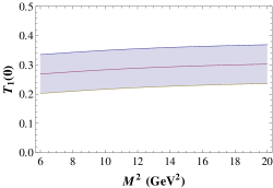
Figure 2: Dependence of $T_{1}^{B^{*}\to K}(0)$ on the Borel parameter $M^{2}$.

For all values of $q^{2}$ in the range $[0,20]$ GeV² the computed form factor is plotted in Fig. 3. The functional $q^{2}$ dependence is obtained fitting the sum rule result by a single pole parametrization:

$$T_{1}^{B^{*}\to K}(q^{2})={T_{1}^{B^{*}\to K}(0)\over 1-\displaystyle{q^{2}\over M_{P}^{2}}}$$ (40)

with

$$T_{1}^{B^{*}\to K}(0)=0.30\pm 0.066\hskip 56.9055ptM_{P}=5.767\,{\rm GeV}\,\,\,.$$ (41)

The uncertainty of $T_{1}^{B^{*}\to K}(0)$ also accounts for the variation of the Borel parameter within the stability window.

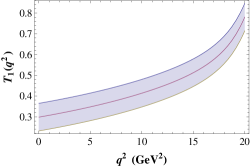
Figure 3: $q^{2}$ dependence of the form factor $T_{1}^{B^{*}\to K}(q^{2})$.

We conclude this section with a comment about the relations among the form factors that parametrize the $B$ to a light meson $L$ matrix elements. As shown in Ref.Charles:1998dr , when the energy of $L$ in the rest-frame of the decaying $B$ meson is large, the form factors describing the $B$ to $L$ transitions can be related among each other. Considering also the heavy quark limit, it is possible to relate the $B\to L$ form factors to the $B^{*}\to L$ ones, as shown in Beneke:2000wa where also the perturbative corrections to the large energy relations have been worked out. In particular, the relation $T_{1}^{B^{*}\to K}=f_{+}^{B\to K}$ should hold for large kaon energy, where $f_{+}$ parametrizes the matrix element of the quark vector current ${\bar{s}}\gamma_{\mu}b$ between the kaon and the $B$ meson as in the first equation in (23). Since large kaon energy means $q^{2}$ close to $q^{2}=0$, one might exploit the relation $T_{1}^{B^{*}\to K}(0)=f_{+}^{B\to K}(0)$, as done in Fajfer:2008zy . Our computed form factor $T_{1}^{B^{*}\to K}$, together with $f_{+}^{B\to K}(0)=0.331\pm 0.041$ determined by LCSR Ball:2004ye , fulfills the relation within the uncertainties.

IV $B\to K\eta^{(\prime)}\gamma$ decay rates and photon spectra

In Secs.II and III we have collected the quantities necessary to evaluate the amplitudes corresponding to the diagrams in Fig. 1. Input parameters are the quark masses, $m_{b}$ already fixed and $m_{s}=0.130$ GeV Colangelo:2000dp , and the CKM matrix elements $V_{tb}=0.99$, $V_{ts}=0.04$ pdg . We do not include the uncertainties on these parameters because they are small with respect to the uncertainties of the other input quantities; moreover, $m_{s}$ plays a negligible role in the final result. We set the renormalization scale at which we compute the coefficient $C_{7\gamma}^{(eff)}$ to $\mu=5$ GeV, close to the $b$ mass.

We can now discuss the branching fraction and the photon spectrum of $B\to K\eta\gamma$ and $B\to K\eta^{\prime}\gamma$ in the SM and in two new physics models with universal extra dimensions described below. We anticipate that such new physics scenarios belong to the class of minimal flavor violation models, therefore the only modification with respect to the SM consists in a different value of the Wilson coefficients in the effective weak Hamiltonian. Therefore, the three cases, the SM and the two UEDs, share common features, namely the hierarchy among the various decay amplitudes and the shape of the photon spectrum.

For what concerns the intermediate states in the $B\to K\eta^{(\prime)}\gamma$ decay amplitudes, the most important contributions are represented by the diagrams (1), (3) and (4) in the case of the $\eta$, while for $\eta^{\prime}$ the first diagram contributes much less than diagrams (3) and (4). This is due to the coupling $g_{K^{*}K\eta}$ which is much larger than $g_{K^{*}K\eta^{\prime}}$: indeed, from the relations in Sec.II we get $g_{K^{*}K\eta}=11\pm 0.1$ and $g_{K^{*}K\eta^{\prime}}=-2.57\pm 0.19$. We only consider a phase $\theta$ between the sum of the first two amplitudes and $A_{3}+A_{4}$; the fifth diagram turns out to be much smaller than the others, hence we assign to it the same phase as $A_{3}$ and $A_{4}$ since a wide change of its phase does not modify the result. In the case of $\eta^{\prime}$ we do not consider the contribution of $K^{*}_{2}$, and $\theta$ is the phase between $A_{1}$ and $A_{3}+A_{4}+A_{5}$. From the calculation of ${\cal B}(B\to K\eta\gamma)$ we shall see that there is a range of values of $\theta$ allowing to reproduce experimental data in Table 1. Let us start from the standard model.

IV.1 $B\to K\eta^{(\prime)}\gamma$ in the standard model

The plot of the computed ${\cal B}(B\to K\eta\gamma)$ as a function of the strong phase $\theta$ is depicted in Fig. 4. The experimental results in Table 1 can be obtained for $\theta=1.8\pm 1.0$ rad, corresponding approximately to $\theta=\left(7\pm 3\right)\frac{\pi}{12}$ (we have considered the range $0\leq\theta\leq\pi$ since the plot is symmetric with respect to $\theta=0$; indeed, in the branching ratio the term proportional to $\sin\theta$ is 2 orders of magnitude smaller than the one proportional to $\cos\theta$).

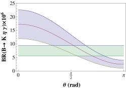
Figure 4: Branching ratio ${\cal B}({\overline{B}^{0}}\to{\overline{K}^{0}}\eta\gamma)$ as a function of the strong phase phase $\theta$ between $A_{1}+A_{2}$ and $A_{3}+A_{4}+A_{5}$. The horizontal band corresponds to the experimental result.

For the central value of $\theta$, the photon spectrum is depicted in Fig. 5. It is peaked at large photon energies and has a structure as the effect of the virtual $K^{*}$. The Dalitz plot in the plane $(M_{\eta K},\,E_{\eta})$, displayed in Fig. 6, also shows the effect of the $K^{*}$ in $B\to K\eta\gamma$, at the limit of the phase space: it should be observed in the data.

In the case of the $\eta^{\prime}$, since the diagram (1) gives a small contribution with respect to (3) and (4), strong phases do not play any role. The result for the branching ratio is ${\cal B}(B\to K\eta^{\prime}\gamma)=(2.78\pm 1.14)\times 10^{-7}$, with the photon spectrum depicted in Fig.5 and the Dalitz plot shown in Fig.6. The theoretical result of the branching fraction for the neutral mode is compatible with the experimental datum in Table 1, which is affected by a large uncertainty. The experimental error is smaller in the charged mode: in this case, while the BaBar result is compatible with the calculation, the Belle measurement is larger. Before commenting on the charged mode, it is worth observing that, for the $B\to K\eta^{(\prime)}\gamma$ three-body channels, the hierarchy between the modes with $\eta$ and $\eta^{\prime}$, observed in data, is reproduced by the theoretical calculation in the frameworks of the QF scheme for the $\eta-\eta^{\prime}$ mixing.

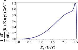
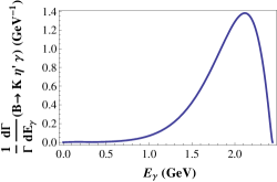
Figure 5: Photon spectrum in ${\overline{B}^{0}}\to{\overline{K}^{0}}\eta\gamma$ (left) and ${\overline{B}^{0}}\to{\overline{K}^{0}}\eta^{\prime}\gamma$ (right). The phase $\theta$ is set to $\theta=1.8$ rad.

Let us discuss the differences between the neutral ${\overline{B}^{0}}$ and the charged $B^{\pm}$ radiative decays. The analysis of the charged modes would be the same as the one we have presented for the neutral modes, except for the contribution of the inner bremsstrahlung diagrams with the photon coupled to the charged initial $B^{+}$ and final $K^{+}$ mesons. The kinematical region in which the bremsstrahlung could be competitive with the other decay mechanisms is for soft photons, due to the presence of a pole at vanishing photon energy. To describe this contribution to the $B^{+}\to K^{+}\eta^{(\prime)}\gamma$ decay, we invoke the Low theorem Low:1958sn which, for scalar particles, allows to relate the amplitude of the radiative mode with a soft photon to the amplitude $A(B^{+}\to K^{+}\eta^{(\prime)})$:

$$A_{IB}(B^{+}(p)\to K^{+}(p_{K})\eta^{(\prime)}(p_{\eta^{(\prime)}})\gamma(q,\epsilon))=e\,\left({\epsilon^{*}\cdot p_{K}\over q\cdot p_{K}}-{\epsilon^{*}\cdot p_{\eta^{(\prime)}}\over q\cdot p_{\eta^{(\prime)}}}\right)\,A(B^{+}\to K^{+}\eta^{(\prime)})\,\,.$$ (42)

The two-body amplitudes in (42) can be determined from the experimental branching fractions ${\cal B}(B^{+}\to K^{+}\eta)=(2.33\pm^{0.33}_{0.29})\times 10^{-6}$ and ${\cal B}(B^{+}\to K^{+}\eta^{\prime})=(7.06\pm 0.25)\times 10^{-5}$ pdg . In the case of the $\eta$, the estimated contribution of the inner bremsstrahlung diagram to the decay rate is of order ${\cal O}(10^{-8})$; therefore, the rate of the charged mode is not significantly affected by this effect, as indeed observed in the data in Table 1. The contribution is more important for the $\eta^{\prime}$: varying the relative phase $\theta_{brem}$ between the bremsstrahlung amplitude and the other considered amplitudes, ${\cal B}(B^{+}\to K^{+}\eta^{\prime}\gamma)$ varies between $(2.3\pm 1.0)\times 10^{-7}$ and $(3.8\pm 1.4)\times 10^{-7}$. These results are within $1\sigma$ from the central value of the BaBar measurement in Table 1, while they deviate by about $2.5\sigma$ from the Belle data. We do not further elaborate on this point: if the deviation is confirmed (or strengthened) by new measurements, the interesting issue of additional contributions to the $B^{+}\to K^{+}\eta^{\prime}\gamma$ amplitude must be addressed.

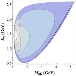
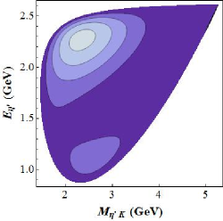
Figure 6: Dalitz plot of ${\overline{B}^{0}}\to{\overline{K}^{0}}\eta\gamma$ (left panel) and ${\overline{B}^{0}}\to{\overline{K}^{0}}\eta^{\prime}\gamma$ (right panel) in the plane $(M_{\eta^{(\prime)}K},E_{\eta^{(\prime)}})$. The photon and the $\eta^{(\prime)}$ energy in the $B$ rest frame are $\displaystyle E_{\gamma}=\left({M^{2}_{B}-M^{2}_{\eta^{(\prime)}K}}\right)/{2M_{B}}$ and $\displaystyle E_{\eta^{(\prime)}}=\left({M^{2}_{B}+M^{2}_{\eta^{(\prime)}}-t}\right)/{2M_{B}}$, respectively. Lighter colors correspond to higher values of the distribution.

IV.2 Sensitivity of $B\to K\eta\gamma$ to two new physics UED scenarios

It is worth investigating the sensitivity of the rare FCNC $B\to K\eta\gamma$ transition to new physics effects. In particular, it is important to establish which kind of improvement can be achieved by a more precise determination of the branching fraction. The considered new physics scenarios involve one or two universal extra dimensions (UED).

The scenario with a single universal extradimension is the Appelquist-Cheng-Dobrescu (ACD) model Appelquist:2000nn , a minimal extension of SM in $4+1$ dimensions, with the extra dimension compactified to the orbifold $S^{1}/Z_{2}$ and the fifth coordinate $y$ running from $0$ to $2\pi R$, $y=0$ and $y=\pi R$ being fixed points of the orbifold. All the fields propagate in all $4+1$ dimensions, therefore the model belongs to the class of universal extra dimension scenarios; one of its motivations is that it naturally provides candidates for the dark matter.

In the ACD model the SM particles correspond to the zero modes of fields propagating in the compactified extra dimension. In addition to the zero modes, towers of Kaluza-Klein (KK) excitations are predicted to exist, corresponding to the higher modes of the fields in the extra dimension; such fields are imposed to be even under a $y\to-y$ transformation in the fifth coordinate. On the other hand, fields which are odd under this transformation propagate in the extra dimension without zero modes, and correspond to particles without SM partners.

The masses of KK particles depend on the radius $R$ of the compactified extra dimension, the new parameter with respect to SM. For example, the masses of the KK bosonic modes are given by

$$m_{n}^{2}=m_{0}^{2}+{n^{2}\over R^{2}}\,\,\,\,\,\,\,n=1,2,\dots$$ (43)

$m_{0}$ being the mass of the zero mode, so that for small values of $R$, i.e. at large compactification scales, the KK particles decouple from the low-energy regime. Another property of the ACD model is the conservation of the KK parity $(-1)^{j}$, $j$ being the KK number. KK parity conservation implies the absence of tree level contributions of Kaluza-Klein states to processes taking place at low energy, forbidding the production of a single KK particle off the interaction of standard particles. This permits to use the electroweak measurements to provide a lower bound to the compactification scale: ${1/R}\geq 250-300$ GeV Appelquist:2002wb . Moreover, this suggests the possibility that the lightest KK particles, namely the $n=1$ Kaluza-Klein excitations of the photon and neutrinos, are among the dark matter components Cheng:2002iz ; Hooper:2007qk .

Since KK modes affect the loop-induced processes, flavor changing neutral current transitions can constrain this new physics scenario. Indeed, many observables are sensitive to the compactification radius in the case, e.g., of processes involving $B$, $B_{s}$ and $\Lambda_{b}$ buras ; noi0 ; noi ; UEDvarie ; UEDvarie1 ; UEDvarie2 . In the ACD model no operators other than those in (II) contribute to $b\to s\gamma$, and the effects beyond SM are only encoded in the Wilson coefficients of the effective Hamiltonian. The contribution of KK excitations modifies in particular the coefficient $C_{7\gamma}$, which acquires a dependence on the compactification scale $1/R$. For large values of $1/R$, due to decoupling of massive KK states, the coefficient $C_{7\gamma}$ (whose explicit expression can be found in buras ) reproduces the standard model value. For this scenario, the bound $\displaystyle\frac{1}{R}>600$ GeV has been established from exclusive noi0 and inclusive UEDvarie radiative rare $B$ decays.

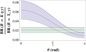
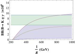
Figure 7: Ratio of the experimental branching fractions $\displaystyle\frac{{\cal B}({\overline{B}^{0}}\to{\overline{K}^{0}}\eta\gamma)}{{\cal B}({\overline{B}^{0}}\to X_{s}\gamma)}$ as a function of the phase $\theta$ (left panel), and branching fraction ${\cal B}({\overline{B}^{0}}\to{\overline{K}^{0}}\eta\gamma)$ computed in the model with two universal extra dimensions as a function of the inverse of the compactification radius (in GeV) and for the phase in the range fixed in (a) (right panel). The horizontal bands correspond to the experimental data.

The second scenario we consider involves two UEDs Dobrescu:2004zi . In this case, the two extra dimensions are flat and compactified on a (so-called chiral) square of side $L$: $0\leq x^{4},x^{5}\leq L$, where $x^{4}$ and $x^{5}$ are the fifth and sixth extra spatial coordinates. The compactification is performed identifying two pairs of adjacent sides of the square: $(y,0)=(0,y)$ and $(y,L)=(L,y)$, for all $y\in[0,L]$, which amounts to folding the square along a diagonal. The fields are decomposed in Fourier modes in terms of effective four dimensional fields labeled by two indices $(l,k)$. Hence, the KK modes are identified by two KK numbers which determine their mass in four dimensions: zero modes corresponds to SM fields. The values of the fields in the points identified through the folding are related by a symmetry transformation. For example, for a scalar field, the field values may differ by a phase. The choice of the folding boundary conditions (and of the constraints on such phases) is mostly important in the case of fermions, since a suitable choice allows to obtain chiral zero modes, while higher KK modes have masses determined (as for scalars) by the relation: $M_{l,k}=\displaystyle{\sqrt{l^{2}+k^{2}}\over R}$, where $R=\displaystyle{L\over\pi}$ is the compactification radius. The theory has an additional symmetry, the invariance under reflection with respect to the center of the square. Such a symmetry distinguishes between the various KK excitations of a given particle. A KK mode identified by the pair $(l,k)$ of indices changes sign under reflection if $l+k$ is odd, while it remains invariant if $l+k$ is even. As a consequence, the stability of the lightest KK modes is guaranteed, and such modes are good candidates for dark matter.

The model comprises the SM particles and their KK excitations, together with new particles without a SM correspondent, described by fields whose Fourier decomposition does not contain a zero mode. Examples are the mixing of the fifth and fourth components of the vector fields and the Higgs fields. All these new particles may contribute as intermediate states in the FCNC loop diagrams and, as in the single UED case, they modify the values of the Wilson coefficient in the effective Hamiltonian (II) without introducing new operators. The explicit expression of $C_{7\gamma}^{eff}$ in this model can be found in Ref.Freitas:2008vh . It should only be mentioned that the sums over the KK modes entering in the expression of the Wilson coefficients in the extra dimensional framework diverge logarithmically, and should be cut in correspondence of some values of $N_{KK}=l+k$, viewing this theory as an effective one valid up to a some higher scale. The condition $N_{KK}\simeq 10$ has been chosen in Freitas:2008vh .

In order to disentangle the dependence of the rate $B\to K\eta\gamma$ on the phase $\theta$ and on the Wilson coefficient $C_{7}$ which encodes the new physics effects, we consider the ratio $\displaystyle\frac{BR({\overline{B}^{0}}\to{\overline{K}^{0}}\eta\gamma)}{BR({\overline{B}^{0}}\to X_{s}\gamma)}$ versus $\theta$, with the experimental datum of $BR({\overline{B}^{0}}\to X_{s}\gamma)$ reported in hfag and the theoretical expression that can be found, e.g. in Ewerth:2009yr . In this ratio, the dependence on $C_{7}$ cancels out, so that we can fix the range of allowed values of the phase depending on the experimental measurements with their own accuracy. As depicted in Fig. 7, the data allow to determine a range for $\theta$ (a strong interaction quantity): $\theta=2.19\pm 0.75$ rad, which is compatible with the range determined in the previous section and can be reduced by improved measurements of the decay rates. With $\theta$ in this range and the expression of $C_{7\gamma}^{eff}$ dependent in both the models on the respective compactification radii, we can compute $BR({\overline{B}^{0}}\to{\overline{K}^{0}}\eta\gamma)$ versus $\displaystyle 1/R$. While for the case of the ACD model no sensible bound on $1/R$ can be worked out, in the case of two UEDs, as plotted in Fig. 7, the constraint $\displaystyle{1\over R}>400$ GeV can be derived. Although such a constraint is weaker than the bound established from the inclusive radiative rare $B$ decay rate, $\displaystyle{1\over R}>650$ GeV Freitas:2008vh , it represents an additional information that can be made more precise, e.g., improving the experimental data.

V Conclusions

$B$ decays to two light pseudoscalar mesons and a photon are interesting, as witnessed by the experimental efforts to determine, for the modes $B\to K\eta^{(\prime)}\gamma$ considered here, the branching fractions and the CP asymmetry parameters. We have studied such channels considering the contribution of amplitudes corresponding to several intermediate states, $K^{*}(892)$ and $K^{*}_{2}(1430)$, as well as $B^{*}$, $B^{*}_{s}$ and $\phi(1020)$. A light cone sum rule determination of the form factor $T_{1}^{B^{*}\to K}(q^{2})$ has been performed: this form factor is of interest since it also enters in other amplitudes involving $B^{*}$ mesons. Introducing a strong phase $\theta$ between the first two considered contributions and the other three, we have shown that the measured $B\to K\eta\gamma$ branching fraction can be reproduced. On the other hand, the experimental uncertainties in ${\cal B}(B\to K\eta^{\prime}\gamma)$ are large, so that the comparison with the theoretical result does not provide constraints, at present. In any case, the modes with $\eta^{\prime}$ in the final state are not enhanced with respect to those with the $\eta$, as experimentally observed. The photon spectrum, as well as the Dalitz plots, are sensitive to the intermediate contributions.

We have studied the radiative transitions in NP scenarios with one and two universal extra dimensions, to study their sensitivity to NP effects. We have found that, in the case of two UEDs compactified on the chiral square, the bound $\displaystyle{1\over R}>400$ GeV can be established from ${\cal B}({\overline{B}^{0}}\to{\overline{K}^{0}}\eta\gamma)$.

Appendix A LCDAs of the $K$ meson

Here we collect the matrix element defining the LCDAs of the kaon used for the calculation of the form factor $T_{1}^{B^{*}\to K}(q^{2})$ .

• Two-particle LCDAs

$$\langle K(p^{\prime})|{\bar{s}}(x)\gamma_{\mu}\gamma_{5}q(0)|0\rangle=-i\,p^{\prime}_{\mu}\int_{0}^{1}due^{i\,up^{\prime}\cdot x}[\phi_{K}(u)+{x^{2}\over 16}\phi_{4K}(u)]-{i\over 2}f_{K}{x_{\mu}\over p^{\prime}\cdot x}\int_{0}^{1}e^{i\,up^{\prime}\cdot x}\psi_{4K}(u)\,\,;$$

$$\langle K(p^{\prime})|{\bar{s}}(x)i\gamma_{5}q(0)|0\rangle={f_{K}m_{K}^{2}\over m_{s}+m_{q}}\int_{0}^{1}due^{i\,up^{\prime}\cdot x}\phi_{P}(u)\,\,;$$

$$\langle K(p^{\prime})|{\bar{s}}(x)\sigma_{\mu\nu}\gamma_{5}q(0)|0\rangle=i\,(p^{\prime}_{\mu}x_{\nu}-p^{\prime}_{\nu}x_{\mu}){f_{K}m_{K}^{2}\over 6(m_{s}+m_{q})}\int_{0}^{1}due^{i\,up^{\prime}\cdot x}\phi_{\sigma}(u)\,\,.$$

• Three-particle LCDAs

$$\langle K(p^{\prime})|{\bar{s}}(x)g_{s}G^{\theta\tau}\sigma_{\rho\nu}\gamma_{5}q(0)|0\rangle=$$

$$i\,f_{3K}[(p^{\prime\theta}p^{\prime}_{\rho}g^{\tau}_{\nu}-p^{\prime\tau}p^{\prime}_{\rho}g^{\theta}_{\nu})-(p^{\prime\theta}p^{\prime}_{\nu}g^{\tau}_{\rho}-p^{\prime\tau}p^{\prime}_{\nu}g^{\theta}_{\rho})]\int{\cal D}\alpha_{i}\phi_{3K}(\alpha_{1},\alpha_{2},\alpha_{3})e^{i\,p^{\prime}\cdot x\,(\alpha_{1}+v\,\alpha_{3})}\,\,;$$

$$\langle K(p^{\prime})|{\bar{s}}(x)g_{s}G^{\theta\tau}\gamma^{\psi}\gamma_{5}q(0)|0\rangle=$$

$$f_{K}\left[p^{\prime\tau}\left(g^{\theta\psi}-{x^{\theta}p^{\prime\psi}\over p^{\prime}\cdot x}\right)-p^{\prime\theta}\left(g^{\tau\psi}-{x^{\tau}p^{\prime\psi}\over p^{\prime}\cdot x}\right)\right]\int{\cal D}\alpha_{i}\,e^{i\,p^{\prime}\cdot x\,(\alpha_{1}+v\,\alpha_{3})}\,\varphi_{\perp}(\alpha_{1},\alpha_{2},\alpha_{3})$$

$$+f_{K}{p^{\prime\psi}\over p^{\prime}\cdot x}(p^{\prime\theta}x^{\tau}-p^{\prime\tau}x^{\theta})\int{\cal D}\alpha_{i}\,e^{i\,p^{\prime}\cdot x\,(\alpha_{1}+v\,\alpha_{3})}\,\varphi_{\parallel}(\alpha_{1},\alpha_{2},\alpha_{3})\,\,;$$

$$\langle K(p^{\prime})|{\bar{s}}(x)g_{s}{\tilde{G}}^{\theta\tau}\gamma^{\psi}q(0)|0\rangle=$$

$$f_{K}\left[p^{\prime\tau}\left(g^{\theta\psi}-{x^{\theta}p^{\prime\psi}\over p^{\prime}\cdot x}\right)-p^{\prime\theta}\left(g^{\tau\psi}-{x^{\tau}p^{\prime\psi}\over p^{\prime}\cdot x}\right)\right]\int{\cal D}\alpha_{i}\,e^{i\,p^{\prime}\cdot x\,(\alpha_{1}+v\,\alpha_{3})}\,{\tilde{\varphi}}_{\perp}(\alpha_{1},\alpha_{2},\alpha_{3})$$

$$+f_{K}{p^{\prime\psi}\over p^{\prime}\cdot x}(p^{\prime\theta}x^{\tau}-p^{\prime\tau}x^{\theta})\int{\cal D}\alpha_{i}\,e^{i\,p^{\prime}\cdot x\,(\alpha_{1}+v\,\alpha_{3})}\,{\tilde{\varphi}}_{\parallel}(\alpha_{1},\alpha_{2},\alpha_{3})\,\,.$$

The following definitions have been used: ${\cal D}\alpha_{i}=d\alpha_{1}d\alpha_{2}d\alpha_{3}\,\delta(1-\alpha_{1}-\alpha_{2}-\alpha_{3})$ and ${\tilde{G}}^{\alpha\beta}={1\over 2}\epsilon^{\alpha\beta\theta\tau}G_{\theta\tau}$. The expressions of the LCDAs listed above, together with the numerical values of the parameters entering in such expressions, can be found in Ball:2006wn . For the sake of clarity, we report below the correspondence between the LCDAs used in this paper and those in Ball:2006wn :

$$\phi_{K}\to\phi_{2;K}\,\,;\hskip 28.45274pt\phi_{4K}\to\phi_{4;K}\,\,;\hskip 28.45274pt\psi_{4K}\to\psi_{4;K}\,\,;$$

$$\phi_{P}\to\phi^{p}_{3;K}\,\,;\hskip 28.45274pt\phi_{\sigma}\to\phi^{\sigma}_{3,K}\,\,;\hskip 28.45274pt\phi_{3K}\to\Phi^{3;K}\,\,;\hskip 28.45274pt$$

$$\varphi_{\parallel}\to\Phi_{4;K}\,\,;\hskip 28.45274pt\varphi_{\perp}\to\Psi_{4;K}\,\,;\hskip 28.45274pt{\tilde{\varphi}}_{\parallel}\to{\tilde{\Phi}}_{4;K}\,\,;\hskip 28.45274pt{\tilde{\varphi}}_{\perp}\to{\tilde{\Psi}}_{4;K}\,\,.$$

References

- (1) M. Artuso, D. M. Asner, P. Ball, E. Baracchini, G. Bell, M. Beneke, J. Berryhill and A. Bevan et al., Eur. Phys. J. C 57, 309 (2008).
- (2) K. Nakamura et al. (Particle Data Group), J. Phys. G 37, 075021 (2010) and http://pdg.lbl.gov/.
- (3) D. Atwood, M. Gronau and A. Soni, Phys. Rev. Lett. 79, 185 (1997); B. Grinstein, Y. Grossman, Z. Ligeti and D. Pirjol, Phys. Rev. D 71, 011504 (2005); D. Atwood, T. Gershon, M. Hazumi and A. Soni, Phys. Rev. D 71, 076003 (2005); B. Grinstein and D. Pirjol, Phys. Rev. D 73, 014013 (2006).
- (4) P. Colangelo and F. De Fazio, Phys. Lett. B 520, 78 (2001).
- (5) H. J. Lipkin, Phys. Lett. B 254, 247 (1991).
- (6) M. Beneke and M. Neubert, Nucl. Phys. B 651, 225 (2003).
- (7) S. Nishida et al. [Belle Collaboration], Phys. Lett. B 610, 23 (2005).
- (8) R. Wedd et al. [Belle Collaboration], Phys. Rev. D 81, 111104 (2010).
- (9) B. Aubert et al. [BABAR Collaboration], Phys. Rev. D 74, 031102 (2006).
- (10) B. Aubert et al. [BABAR Collaboration], Phys. Rev. D 79, 011102 (2009).
- (11) S. Fajfer, T. N. Pham and N. Kosnik, Phys. Rev. D 78, 074013 (2008).
- (12) G. Buchalla, A. J. Buras and M. E. Lautenbacher, Rev. Mod. Phys. 68, 1125 (1996).
- (13) A. J. Buras, P. Gambino and U. A. Haisch, Nucl. Phys. B 570, 117 (2000); M. Gorbahn and U. Haisch, Nucl. Phys. B 713, 291 (2005); M. Misiak et al., Phys. Rev. Lett. 98, 022002 (2007). For a comprehensive review on the status of the calculation of the Wilson coefficients see: A. J. Buras, arXiv:1102.5650 [hep-ph].
- (14) A. J. Buras, M. Misiak, M. Munz and S. Pokorski, Nucl. Phys. B 424, 374 (1994).
- (15) T. Feldmann, P. Kroll and B. Stech, Phys. Rev. D 58, 114006 (1998) and Phys. Lett. B 449, 339 (1999); T. Feldmann, Int. J. Mod. Phys. A 15, 159 (2000).
- (16) F. De Fazio and M. R. Pennington, JHEP 0007, 051 (2000).
- (17) F. Ambrosino et al. [KLOE Collaboration], Phys. Lett. B 648, 267 (2007).
- (18) F. Ambrosino et al., JHEP 0907, 105 (2009).
- (19) M.B. Wise, Phys. Rev. D 45, R2188 (1992); G. Burdman and J.F. Donoghue, Phys. Lett. B 280, 287 (1992); P. Cho, Phys. Lett. B 285, 145 (1992); H.-Y. Cheng et al., Phys. Rev. D 46, 1148 (1992); R. Casalbuoni, A. Deandrea, N. Di Bartolomeo, R. Gatto, F. Feruglio and G. Nardulli, Phys. Rept. 281, 145 (1997).
- (20) P. Colangelo, G. Nardulli, A. Deandrea, N. Di Bartolomeo, R. Gatto and F. Feruglio, Phys. Lett. B 339, 151 (1994); P. Colangelo, F. De Fazio and G. Nardulli, Phys. Lett. B334, 175 (1994); V. M. Belyaev, V. M. Braun, A. Khodjamirian and R. Ruckl, Phys. Rev. D 51, 6177 (1995); P. Colangelo, F. De Fazio, G. Nardulli, N. Di Bartolomeo and R. Gatto, Phys. Rev. D 52, 6422 (1995); P. Colangelo and F. De Fazio, Eur. Phys. J. C 4, 503 (1998); D. Becirevic, B. Blossier, E. Chang and B. Haas, Phys. Lett. B 679, 231 (2009).
- (21) A. Anastassov et al. [CLEO Collaboration], Phys. Rev. D 65, 032003 (2002).
- (22) A discussion can be found in P. Colangelo and F. De Fazio, Phys. Lett. B 532, 193 (2002).
- (23) P. Ball and R. Zwicky, Phys. Rev. D 71, 014015 (2005).
- (24) P. Colangelo, F. De Fazio and G. Nardulli, Phys. Lett. B 334, 175 (1994).
- (25) P. Colangelo and A. Khodjamirian, in “At the Frontier of Particle Physics / Handbook of QCD“, ed. by M. Shifman (World Scientific, Singapore, 2001), vol. 3, 1495-1576, [hep-ph/0010175].
- (26) P. Ball and R. Zwicky, Phys. Rev. D 71, 014029 (2005).
- (27) P. Colangelo, F. De Fazio, P. Santorelli and E. Scrimieri, Phys. Rev. D 53, 3672 (1996) [Erratum-ibid. D 57, 3186 (1998)].
- (28) W. Wang, Phys. Rev. D 83, 014008 (2011).
- (29) M. A. Shifman, in “At the Frontier of Particle Physics / Handbook of QCD“, ed. by M. Shifman (World Scientific, Singapore, 2001), vol. 3, 1447-1494, [hep-ph/0009131].
- (30) P. Ball, V. M. Braun and A. Lenz, JHEP 0605, 004 (2006).
- (31) A. Khodjamirian, R. Ruckl, S. Weinzierl and O. I. Yakovlev, Phys. Lett. B 457, 245 (1999).
- (32) J. Charles, A. Le Yaouanc, L. Oliver, O. Pene and J. C. Raynal, Phys. Rev. D 60, 014001 (1999).
- (33) M. Beneke and T. Feldmann, Nucl. Phys. B 592, 3 (2001).
- (34) F. E. Low, Phys. Rev. 110, 974 (1958).
- (35) T. Appelquist, H. C. Cheng and B. A. Dobrescu, Phys. Rev. D 64, 035002 (2001).
- (36) I. Antoniadis, Phys. Lett. B 246, 377 (1990).
- (37) T. Appelquist and H. U. Yee, Phys. Rev. D 67, 055002 (2003).
- (38) H. C. Cheng, K. T. Matchev and M. Schmaltz, Phys. Rev. D 66, 036005 (2002), Phys. Rev. D 66, 056006 (2002); G. Servant and T. M. P. Tait, Nucl. Phys. B 650, 391 (2003).
- (39) For a review see: D. Hooper and S. Profumo, Phys. Rept. 453, 29 (2007).
- (40) A. J. Buras, M. Spranger and A. Weiler, Nucl. Phys. B 660, 225 (2003); A. J. Buras, A. Poschenrieder, M. Spranger and A. Weiler, Nucl. Phys. B 678, 455 (2004).
- (41) P. Colangelo, F. De Fazio, R. Ferrandes and T. N. Pham, Phys. Rev. D 73, 115006 (2006).
- (42) P. Colangelo, F. De Fazio, R. Ferrandes and T. N. Pham, Phys. Rev. D 74, 115006 (2006); Phys. Rev. D 77, 055019 (2008). M. V. Carlucci, P. Colangelo and F. De Fazio, Phys. Rev. D 80, 055023 (2009);
- (43) U. Haisch and A. Weiler, Phys. Rev. D 76, 034014 (2007).
- (44) R. Mohanta and A. K. Giri, Phys. Rev. D 75, 035008 (2007); T. M. Aliev and M. Savci, Eur. Phys. J. C 50, 91 (2007); T. M. Aliev, M. Savci and B. B. Sirvanli, Eur. Phys. J. C 52, 375 (2007); I. Ahmed, M. A. Paracha and M. J. Aslam, Eur. Phys. J. C 54, 591 (2008); A. Saddique, M. J. Aslam and C. D. Lu, Eur. Phys. J. C 56, 267 (2008); V. Bashiry and K. Zeynali, Phys. Rev. D 79, 033006 (2009); Y. M. Wang, M. J. Aslam and C. D. Lu, Eur. Phys. J. C 59, 847 (2009).
- (45) G. Devidze, A. Liparteliani and U. G. Meissner, Phys. Lett. B 634, 59 (2006); I. I. Bigi, G. G. Devidze, A. G. Liparteliani and U. G. Meissner, Phys. Rev. D 78, 097501 (2008).
- (46) B. A. Dobrescu and E. Ponton, JHEP 0403, 071 (2004); G. Burdman, B. A. Dobrescu and E. Ponton, JHEP 0602, 033 (2006).
- (47) A. Freitas and U. Haisch, Phys. Rev. D 77, 093008 (2008).
- (48) D. Asner et al., "Averages of b-hadron, c-hadron, and tau-lepton Properties," arXiv:1010.1589 and online update at http://www.slac.stanford.edu/xorg/hfag
- (49) T. Ewerth, P. Gambino and S. Nandi, Nucl. Phys. B 830, 278 (2010).