The Spitzer Spectroscopic Survey of S-type Stars

Abstract

Context. S-type AGB stars are thought to be in the transitional phase between M-type and C-type AGB stars. Because the composition of the circumstellar environment reflects the photospheric abundances, one may expect a strong influence of the stellar C/O ratio on the molecular chemistry and the mineralogy of the circumstellar dust.

Aims. In this paper, we present a large sample of 87 intrinsic galactic S-type AGB stars, observed at infrared wavelengths with the Spitzer Space Telescope, and supplemented with ground-based optical data.

Methods. On the one hand, we derive the stellar parameters from the optical spectroscopy and photometry, using a grid of model atmospheres. On the other, we decompose the infrared spectra to quantify the flux-contributions from the different dust species. Finally, we compare the independently determined stellar parameters and dust properties.

Results. For the stars without significant dust emission features, we detect a strict relation between the presence of SiS absorption in the Spitzer spectra and the C/O ratio of the stellar atmosphere. These absorption bands can thus be used as an additional diagnostic for the C/O ratio. For stars with significant dust emission, we define three distinct groups, based on the relative contribution of certain dust species to the infrared flux. We find a strong link between group-membership and C/O ratio. Furthermore, we show that these groups can be explained by assuming that the dust-condensation can be cut short before silicates are produced, while the remaining free atoms and molecules can then be used to form the observed magnesium sulfides or the carriers of the unidentified 13 $\mu$m and 20 $\mu$m features. Finally, we present the detection of emission features attributed to molecules and dust characteristic to C-type stars, such as molecular SiS, hydrocarbons and magnesium sulfide grains. We show that we often detect magnesium sulfides together with molecular SiS and we propose that it is formed by a reaction of SiS molecules with Mg.

1 Introduction

The dredge-up of carbon in asymptotic giant branch (AGB) stars plays a key role in the chemical evolution from oxygen-rich M-type stars to carbon-rich C-type stars (Iben & Renzini, 1983; Herwig, 2005; Habing & Olofsson, 2004). S-type stars are often considered to be an intermediate phase of AGB evolution between M- and C-type stars in which the C/O ratio of stars changes from the solar value to ratios larger than unity. In the spectral classification scheme, S-type stars are defined by the presence of absorption bands of ZrO and LaO molecules in the optical spectra. The transition from oxygen-rich to carbon-rich marks an important chemical transition in the AGB evolution.

Following the chemical pathways relevant in the circumstellar environment, CO is the first molecule to form, locking up all of the available carbon or oxygen, whichever is less abundant. Subsequently, in M-type stars (C/O $<$ 1) almost all C atoms will be consumed by CO and oxygen-rich molecules such as TiO, SiO, and H₂O will be present. In carbon-rich stars (C/O $>$ 1) the dominant molecules are CO, CH, C₂, and C₂H₂. However, it is important to realize that this is a simplified picture of the circumstellar chemistry and only valid under the assumption of local thermal equilibrium (LTE). Due to non-equilibrium chemistry effects, oxygen-rich stars could display molecules that are typical for carbon-rich stars and vice versa (Cherchneff, 2006) .

The chemical and physical properties of circumstellar dust grains are linked to the chemical composition of the stellar atmosphere. In an oxygen-rich environment, silicates and oxides are formed, while graphite, amorphous carbon, and silicon carbide are formed in carbon-rich environments. When the C/O ratio is very close to unity, both O and C are almost completely consumed in CO, in which case the dust condensation sequence is not well studied nor understood. Theoretical models predict the presence of FeSi and metallic Fe, but this still needs observational confirmation (Ferrarotti & Gail, 2002). Furthermore, some molecules and dust species that contain neither C nor O are also limited to certain chemical environments, for example magnesium sulfide dust and SiS molecules are typical for carbon-rich environments. This indicates that the C/O ratio does not only influence the carbon- and oxygen-abundance, but indirectly effects the entire chemical network, of which only a couple of molecular products are detected.

The chemistry of the circumstellar material is key to understanding the driving mechanism of mass-loss in AGB stars, one of the major open questions in stellar evolution. It is generally accepted that the mass loss of AGB stars is dust-driven (Lamers & Cassinelli, 1999). Pulsations bring the envelope far from the stellar equilibrium radius, where the temperatures are low enough for dust-condensation. This dust is easily accelerated by radiative pressure and it drags the gas along. For carbon-rich stars, the opacity of amorphous carbon is high enough in the near-infrared to drive mass loss. For oxygen-rich stars however, theoretical studies suggest that silicates are not able to drive the wind (Woitke, 2006; Höfner & Andersen, 2007; Höfner, 2008). It is clear that an exact understanding of the process is lacking.

A recent study of the infrared spectra of nine S-type AGB stars from the Short Wavelength Spectrometer onboard of the Infrared Space Observatory (ISO/SWS), presented by Hony et al. (2009) showed that the infrared spectra of S-type AGB stars can be significantly different from those of oxygen-rich AGB stars and already reported on the detection of dust emission at 28 $\mu$m attributed to magnesium sulfides. Although this study shows that S-type AGB stars exhibit several unique dust characteristics, the study is limited because ISO/SWS is only sensitive to the brightest (at infrared wavelengths) AGB stars and thus to the S-type stars with higher mass-loss rates, while a large and homogeneous sample is necessary to draw conclusions about the dust condensation in S-type stars.

In this paper we present a combination of optical spectroscopy, infrared photometry and infrared spectroscopy for a sample of 87 intrinsic S-type stars. This sample allows us to study the interaction between the chemistry and dynamics of the stellar atmosphere and the dusty circumstellar environment. In §2 and §3 we discuss the sample selection procedure and the data reduction. In §4 we derive the chemical and variability characteristics of the stars in our sample. In §5 we give an overview of the “naked” stellar atmospheres and we show that their spectral appearance of depends strongly on the C/O ratio of the star. In §6 we present a tool to decompose infrared (IR) spectra into the contribution of the stellar atmosphere and the different dust species, allowing us to classify the IR spectra of dust-rich stars into three distinct groups. We show that there is a relation between the C/O ratio and those groups.

2 The sample of S-type AGB stars

In order to study the interaction between the stellar atmosphere and the infrared properties of S-type AGB stars, we selected a large sample of S-type stars designed to include all intrinsic S-type AGB stars bright enough to be detectable with the Spitzer IRS spectrograph. This sample spans the entire range of C/O ratios, temperatures and s-process abundances found in S-type AGB stars, but is slightly biased towards stars with lower mass-loss rates (see Sect. 2.3).

2.1 Sample selection

A first sample was drawn from the second edition of the General Catalog of S stars (GCSS2, Stephenson, 1994). This catalog classifies 1346 stars as S-type stars, based on the presence of ZrO or LaO bands in the red part of the optical spectrum. This method only selects stars based on an enrichment of s-process elements in their lower envelope, which not only includes stars that have undergone a recent third dredge-up event, the intrinsic S stars, but also stars that are enhanced with s-process elements by binary interaction, called extrinsic S stars (Brown et al., 1990). In order to study the dust-sequence on S-type AGB stars, we need to exclude the extrinsic stars from our sample.

Several properties distinguish both groups, such as luminosity, the $K-[12]$ color, the presence of technetium in the atmosphere, and variability (Van Eck & Jorissen, 1999). The best distinction method is based on the presence of technetium (Tc), which is brought to the surface during the third dredge-up events. With a laboratory half-life time of approximately $2\times 10^{5}$ years, the detection of Tc in the spectrum points to a recent third dredge-up event. Although the detection of Tc is the most secure way to include only intrinsic stars in the sample, it requires high resolution spectroscopy in the blue region where these cool stars are faint. A criterion based on the luminosity would introduce strong and unwanted biases on the distance or intrinsic brightness of the stars, while putting a lower limit on the infrared color $K-[12]$ would favor stars with a dusty circumstellar environment. Considering all this, source variability turns out to be the most efficient way to discriminate between intrinsic and extrinsic S-type stars.

The ASAS light curves of the sample presented by Van Eck et al. (2000) were examined in the light of the intrinsic/extrinsic classification of these authors. For the extrinsic stars (excluding the symbiotic binaries), we found an upper limit of 0.12 mag for the standard deviations of the $V$-band light curves. Hence applying a lower limit of 0.12 mag on the standard deviations of the $V$-band light curves should result in the exclusion of the extrinsic S-type AGB stars. The remaining sample consisted of 459 presumably intrinsic S-type stars with variability amplitudes larger than 0.12 mag.

To estimate the source variability of the S-type stars, we have cross-identified all stars in the GCSS2 with the two major available variability surveys: the All Sky Automated Survey (ASAS) located at the Las Campanas Observatory (Pojmanski et al., 2005) and the Northern Sky Variability Survey (NSVS) operated at Los Alamos National Laboratory (Woźniak et al., 2004a). This resulted in 1154 S-type stars with V-band light curves.

In the last step, the sample was reduced to contain only stars that could be observed by Spitzer within a reasonable integration time. Therefore we used a cross-identification of the remaining sources with the catalogues of the Infrared Astronomical Satellite (IRAS) and the Two Micron All Sky Survey (2MASS). From the relation between the $K$ magnitude and the 12 $\mu$m IRAS flux we estimate that S stars with $4.5\,\mathrm{mag}<K<5.5\,\mathrm{mag}$ exhibit maximum fluxes between 0.3 and 3 Jy in the Spitzer wavelength range, not so bright as to saturate the detector but sufficiently bright to allow short integration times. The final target list contained 90 sources (3 of which will be rejected based on the ground-based optical spectra).

2.2 Extrinsic intruders in our sample

Because the cut-off criterion on the standard deviations of the V-band light curve is not strict, we can expect a small number of extrinsic S-type stars in our sample. As said in the previous section, the best way to (a posteriori) confirm that a star is an S-type AGB star is to check for the presence of the 4238 Å , 4262 Å  and 4297 Å Tc lines in high-resolution spectra (Uttenthaler et al., 2007).

As a filler program, we obtained high-resolution spectra for some of the brightest stars in our sample. The target selection was inhomogeneous, focussing on (i) stars with low-amplitude light curves and (ii) stars with an unusual appearance in the low-resolution optical spectra. The first group of stars was targeted because the chance of finding an extrinsic S-type star amongst the low-amplitude pulsators is larger since true AGB stars are expected to have larger pulsation amplitudes. The stars with an unusual low-resolution optical spectrum could be mis-classified as S-type stars in the GCSS2 (Stephenson, 1994) (e.g. BD$+$02~4571). For more information on the low- and high-resolution spectra and the lightcurves, see Sect. 3.

As shown by Uttenthaler et al. (2007), we can make the distinction between Tc-rich and Tc-poor stars by comparing the flux ratios in the Tc line to a pseudo-continuum flux. Using this method a reliable distinction of this kind can be made, even for low SNR spectra.

Three stars did not show significant Tc lines and were removed from our sample (CPD$-$19~1672, BD$+$02~4571 and CSS~718). Because of the inhomogeneous subset of stars with high-resolution spectra, this ratio of 3 stars without Tc lines in a subset of 13 stars is not representative for the entire sample. Discarding these stars, we are left with a total sample of 87 S-type AGB stars.

2.3 Bias towards low mass-loss rates

During the target selection phase, we put a limit on the $K$-band magnitude and cross-identified the sample with the ASAS and NSVS catalogs. Because both surveys are limited to $V$-band magnitudes of approximately 14 and the $K$-band magnitude is limited to the 4.5–5.5 mag range, we have effectively limited the sample to stars with $V-K<10\,\mathrm{mag}$.

Based on the marcs model atmospheres for S-type AGB stars without detectable circumstellar material (see Section 4), we can expect $V-K$ values up to 10 mag or more for stars with $T_{\mathrm{eff}}$ lower than 2700 K, even without circumstellar material. Stars with circumstellar dust are reddened and thus have higher values for the $V-K$ color. The limitation on this color will exclude the stars with the highest mass-loss rates because they appear redder (Guandalini, 2010).

In Fig. 1, we show the $J-K$ and $V-K$ colors for our stars, the sample of S stars observed with ISO/SWS (Hony et al., 2009) and all S-type stars found in the Stephenson Catalog for comparison. For our stars, the phase-calibrated $V$-band magnitudes are derived from the light curves in the ASAS or AAVSO database and new measurements with the MkII photometer, discussed in more detail in Sect. 3.2.1. For the ISO/SWS sources we use the AAVSO database to derive the phase-calibrated $V$ magnitudes. The relations presented in Carpenter (2001) were used to convert the $K_{\mathrm{2MASS}}$ magnitudes to $K_{\mathrm{SAAO}}$ magnitudes. For the S-type stars found in the Stephenson catalog that are not observed with Spitzer or ISO/SWS, the $V-K$ and $J-K$ colors are not phase-calibrated and not corrected for the interstellar reddening because the distances and pulsation characteristics are very uncertain.

From this figure, we can see that although we have indirectly removed stars with $V-K>10\,\mathrm{mag}$ from our sample, this effect is only small and we excluded only the coolest stars which have high mass-loss rates, less than 5% of all S-type stars. Furthermore, the figure shows that the sample of S-type AGB presented in Hony et al. (2009) is biased towards higher mass-loss rates, because the limited sensitivity of the ISO/SWS spectrograph favors stars with a strong infrared excess. We have to keep both biases in mind when we compare our results with literature.

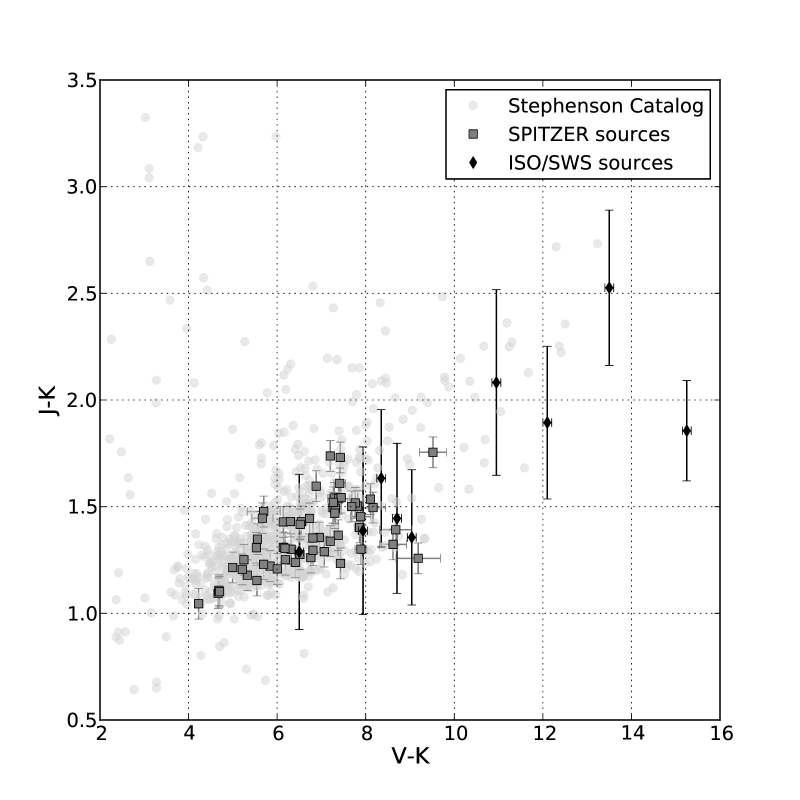
Figure 1: The $V-K$ vs. $J-K$ diagram of the S-type stars in the Stephenson catalog (light grey dots), the ISO/SWS targets presented in Hony et al. (2009) (black diamonds) and the Spitzer sample presented in this paper (dark grey squares).

3 Data

3.1 Spitzer Space Telescope

The IRS data of all 90 S-type stars were obtained using the IRS Standard Staring mode. The targets were observed in two positions in each aperture (SL1, SL2, LL1 and LL2) to obtain low-resolution spectra over the entire wavelength range (5–38 $\mu$m). All data were taken during a period from September 2006 to October 2007 (Program ID 30737, P.I. S. Hony).

For the data reduction we used the FEPS pipeline, developed for the Spitzer legacy program “Formation and evolution of planetary systems”. A detailed description can be found in Hines et al. (2005). For the extraction we start from the intermediate droop data products as delivered by the Spitzer Science Center, together with the SMART reduction package tools described in detail in Higdon et al. (2004). The spectra were extracted using a fixed width aperture, so that 99% of the source flux falls within the aperture. After the extraction of the spectrum for each nod position and cycle, a mean spectrum over all slit positions and cycles is computed for each individual order. Thereafter, the orders are combined. In regions where there is order overlap, the fluxes are replaced by the mean flux value at each wavelength point. The IRSFRINGE package was used for the de-fringing of the spectra. For the calibration, spectral response functions were calculated from standard stars and corresponding stellar models. The estimated average uncertainty on the spectral response function and uncertainty on the extracted spectra are incorporated in the final estimated error. Finally, for each target a one-dimensional spectrum is computed by stitching together overlapping orders. This is done by multiplying the LL orders with a correction factor to match the mean flux with the SL orders in the overlapping wavelength range. No wavelength shifting or spectral tilting is performed.

3.2 Additional ground-based data

3.2.1 SAAO

For 69 of the 87 stars in our sample, we have obtained JHKL magnitudes (1.25, 1.65, 2.2 and 3.5 $\mu$m) at the South African Astronomical Observatory (SAAO). The observations were made with the MkII infrared photometer on the 0.75-m telescope. The accuracy is typically better than 0.03 mag in the J, H, and K band, and better than 0.05 mag in the L band. All JHKL magnitudes derived for these stars are given in Table LABEL:table:data.

3.2.2 Low-resolution optical spectra

Low resolution optical spectra were obtained for 81 of the 87 stars in our sample. The southern objects were observed with the 1.9-m telescope at SAAO, whereas the more northern objects were observed with the ISIS spectrograph mounted on the 4.2-m William Herschel Telescope (WHT) at the Observatory de Roque de los Muchachos (ORM) situated at La Palma.

The spectra were wavelength calibrated with a CuNe+CuAr lamp. The correction for atmospheric extinction was performed using the average curve for the local, continuous atmospheric extinction at the site. The resulting SAAO spectra cover the 4800-7700$\,\AA$ range with a resolving power of $\mathrm{R}=\frac{\lambda}{\Delta\lambda}\approx 3800$. The spectra of WHT consist of a blue arm, spanning 3700-5350$\,\AA$ with a resolving power of $\mathrm{R}\approx 5000$ and a red arm, spanning 5100-8100$\,\AA$ with a resolving power of $\mathrm{R}\approx 3800$.

3.2.3 High-resolution optical spectra

We obtained high-resolution spectra for some of the brightest targets in our sample. Eight southern sources were observed with the Coralie échelle spectrograph at the Euler telescope in La Silla, spaning 3900-6800$\,\AA$, with a resolving power of $\mathrm{R}\approx 50\,000$. Thirteen northern sources were observed with the HERMES échelle spectrograph at the Mercator telescope in La Palma (Raskin et al., 2011), covering 3770-9000$\,\AA$ with a resolving power of $\mathrm{R}\approx 85\,000$. We use the end-products of the automatic data reduction pipelines for both instruments.

3.2.4 Dereddening

To remove the effects of interstellar, wavelength dependent extinction from the ground-based and Spitzer data, we start from the 3-dimensional reddening models of Drimmel et al. (2003) and Marshall et al. (2006). The Marshall model returns the K-band extinction for over 64 000 lines of sight, each separated by $15^{\prime}$, based on the 2MASS point source catalogue. When possible, we use this model to estimate the extinction, but the Marshall model only covers the inner Galaxy ($|l|\leq 100^{\circ},|b|\leq 10^{\circ}$). The model presented in Drimmel et al. (2003) returns V-band extinctions for the entire sky. The data are dereddened, using the extinction laws of Cardelli et al. (1989) for the optical and NIR data and Chiar & Tielens (2006) at longer wavelengths.

4 Stellar parameters

Because the spectral appearance of S-type AGB stars depends strongly on the stellar parameters such as ${\rm T}_{\rm eff}$, C/O ratio, s-process element abundance and iron abundance, it is possible to constrain these stellar parameters by comparing model atmospheres to observational data. These stellar parameters characterize the chemical conditions in the stellar atmosphere. Especially the C/O ratio is expected to have a very profound impact.

Because the sample selection is based on the ASAS and NSVS catalogs, we are able to constrain the pulsation characteristics of most stars. The period and amplitude of the V-band variations characterize the variability of the stellar atmosphere.

4.1 Chemical characterization

4.1.1 Comparison with MARCS model atmospheres

The stellar parameters were derived using a grid of model atmospheres specially computed for S-type stars with the marcs code (Gustafsson et al., 2008). This model grid has been described in Van Eck et al. (2010) and Neyskens et al. (2010). The full detailed description will be published in a forthcoming paper (Plez et al., in preperation). To summarize briefly, the grid covers the following parameter space:

• $2700\leq T_{\rm eff}$ (K) $\leq 4000$ in steps of 100 K

• C/O = 0.5, 0.750, 0.899, 0.925, 0.951, 0.971, 0.991

• $[\rm{s}/\rm{Fe}]$ = 0, +1, +2 dex

• $[\rm{Fe}/\rm{H}]$ = -0.5, 0 dex.

The unequal C/O spacing has been designed to cover in an optimal way the change of the absorption features affecting the optical spectra when C/O increases from 0.5 to unity. All models were computed for a stellar mass of $M=1\,M_{\odot}$ and with $[\alpha/\rm{Fe}]\leavevmode\nobreak\ =-0.4\leavevmode\nobreak\ \times\leavevmode\nobreak\ [\rm{Fe}/\rm{H}]$. It is essential to take into account the non-solar C/O ratio of S-type stars since it has an important impact on the partial pressures of H₂O and TiO, two major opacity contributors. Coupled with s-process overabundances, it affects the depth of the prominent ZrO bands observed in S-type stars. The effect of the gravity was found to be too degenerate to be constrained solely with the observational data available for the present study. Therefore it was fixed in the following way, devised to approximately follow the portion of the AGB covered by the S stars under consideration: $\log{g}=0$ if $T_{\rm eff}<3400$ K, $\log{g}=1$ otherwise. Similarly, low-resolution spectra do not allow to lift the degeneracy between metallicity and s-process overabundance.

A set of well-chosen photometric and narrow-band indices were then computed on the basis of low-resolution synthetic and observed spectra (see Van Eck et al. (2010) for more details). The low-resolution spectra used here consist of Boller & Chivens spectra ($\Delta\lambda=3$ Å, $4400-8200$ Å), SAAO spectra ($\Delta\lambda=1.8$ Å, $4800-7700$ Å) and WHT spectra ($\Delta\lambda=1.8$ Å, $5100-8100$ Å). Two colour indices $V-K$ and $J-K$ as well as three spectroscopic indices (strengths of the carefully-selected ZrO and TiO bands, as well as the strength of the Na D lines) were used to define a total of five indices.

Chi-square minimization between observed and synthetic indices then led to a set of plausible physical parameters (effective temperature, gravity, metallicity, C/O ratio, and [s/Fe]). The agreement between selected synthetic spectra and the observed optical and infrared low-resolution spectra is in most cases very good. However, it is sometimes difficult to select one out of the first few “best-matching” synthetic spectra. In fact, the uncertainties inherent to the whole procedure (e.g., non-simultaneous photometry and spectroscopy, stellar variability, or approximate values of the reddening) have to be taken into account in estimating the best model and the uncertainty on the stellar parameters. The resulting value and uncertainties on the stellar parameters $T_{\rm eff}$, C/O, and [s/Fe] that provide a reasonably good fit between the low-resolution observed and synthetic spectra are given in Table 4.

4.1.2 Stellar properties

From the results in Table 4 we can get a general overview of the chemical properties of the stars in our sample. The effective temperature spans a range from 2900 K for the coolest S-type star to 3650 K for the hottest one, with most stars with $T_{\rm eff}$ around 3300 K. There is a strong correlation between the place in the ZrO–TiO plot and the C/O ratio. The ZrO and TiO indices can thus be used as indirect indicators for the C/O ratio (see Fig. 2). We will make use of this relation throughout the entire paper. The figure shows that one can separate two groups, stars with a low C/O ratio are located at the upper left corner and the stars with a high C/O ratio towards the lower right corner. The position in this diagram can thus be used as a decent estimate for the C/O ratio.

From this figure, we can also see that there is a significant correlation between the [s/Fe] values and the C/O ratios. This obvious correlation was predicted and observationally confirmed in AGB stars (Smith & Lambert, 1990; Mowlavi, 1997) and S-type stars in particular (Van Eck et al., 2010). Because all combinations of C/O and [s/Fe] were allowed, the presence of the relation is not inherent to the method to derive the stellar parameters, but rather shows that the method works well and can reproduce this relationship.

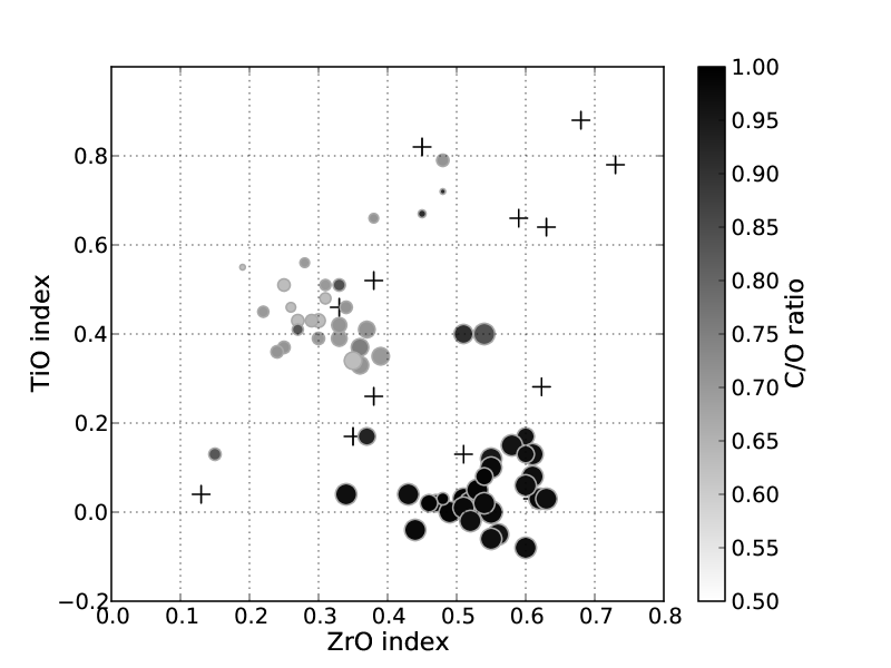
Figure 2: The average line-to-continuum-ratios of the ZrO and TiO absorption bands within the spectral range of WHT and SAAO low-resolution spectra (i.e. ZrO and TiO indices) for all stars in the sample. The size of the symbols increases with [s/Fe] and the color varies with C/O. Crosses indicate stars for which $\mathrm{T_{eff}}$, C/O and [s/Fe] are unknown.

4.2 Variability characterization

To derive the pulsation parameters, we use the databases of NSVS and ASAS. A complete description of the instruments and reduction processes can be found in Woźniak et al. (2004b) and Pojmański (2004). For some stars, additional $V$-band light curves are available from the American Association of Variable Star Observers (AAVSO).

Because for most stars only a few data-points are available, we use the generalized least-squares periodogram to find the pulsation periods of all stars (Zechmeister & Kürster, 2009). This periodogram takes into account that for small datasets the sample average can differ significantly from the true average. Some semi-regular variables are known to exhibit long secondary periods (LSP), typically 5 to 15 times longer than the primary period. When detected, such variations are removed (prewhitened) from the light curve and the period analysis is repeated. The results of this analysis can be found in Table 3.

The period analysis resulted in detected periods for 54 of the 87 stars in our sample. For most cases where no significant periodicity was found, this can be explained by the short timespan of the NSVS light curves. These short timespans allow an identification of the amplitude of the variations, but a period analysis needs longer timespans. For eight stars, the lack of periodicity is due to intrinsic irregular behavior.

In addition to these periods, the General Catalog of Variable Stars (GCVS) gives the period to 18 stars. For 11 of these stars, we also derived a period, based on the NSVS, ASAS and AAVSO light curves. As shown in Table 3, the derived period for 10 of these 11 stars is in close agreement with the periods shown in the GCVS. However, the recent data shows that V899~Aql has a period of 374 days and is most likely a Mira, this star is classified as a semi-regular variable in the GCVS, with a period of 100 days. In further calculations, we will use the periods and pulsation types derived from the NSVS, ASAS, and AAVSO light curves if available. The sample contains 6 irregular pulsators, 38 semi-regular variables and 21 Miras.

5 Naked stellar atmospheres

The 87 S-type stars in our sample show a wide variety of features in the infrared spectra. Some stars show clear dust/molecular emission features, while others only show the molecular absorption features typical for “naked” stellar atmospheres. Because stars with and without emission features have to be treated separately, we classify the targets into naked stellar atmospheres and stars with additional emission features. Out of the 87 stars, 47 are classified as naked stellar atmospheres. The other stars show relatively strong emission features on top of these stellar atmospheres which are due to (i) molecular emission from extended atmospheres (3 stars), (ii) the typical emission features from hydrocarbons (4 stars) or (iii) dust emission (32 stars). Here, we focus on the naked stellar atmospheres. The dust emission will be discussed in more detail in Sect. 6 and the molecular emission in Sect. 7.

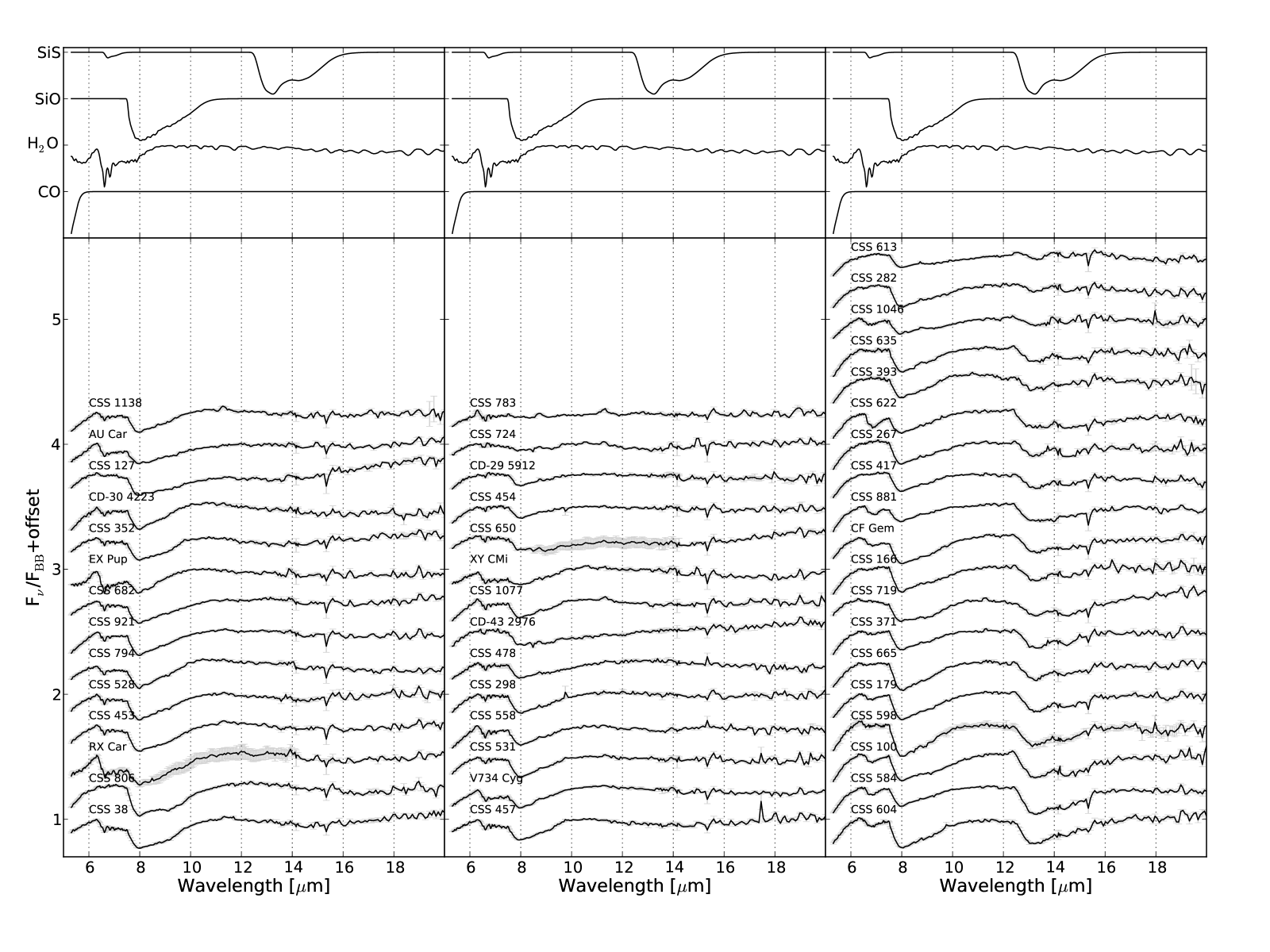
Figure 3: Top panel: the template spectra of SiS, SiO, H₂O, and CO. Bottom panel: the spectra of all naked stars from 5 $\mu$m to 20 $\mu$m, normalized with a blackbody spectrum. The the two panels on the left show the stars without SiS, the right-most panel shows all stars with significant SiS absorption. The sharp feature at 15.3 $\mu$m seen in all stars is most likely an artifact of the data reduction process.

5.1 Overview of the observed absorption bands

In the bottom panel of Fig. 3 we show the normalized infrared spectra of all 47 naked stellar atmospheres of our sample; the top panel shows the normalized templates used for comparison. These templates have column densities and temperatures that are representative for AGB stars (CO at $T=2000\,\mathrm{K}$ and $N=10^{21}\,\mathrm{cm}^{-2}$; H₂O at $T=1500\,\mathrm{K}$ and $N=10^{20}\,\mathrm{cm}^{-2}$; SiO at $T=2000\,\mathrm{K}$ and $N=10^{21}\,\mathrm{cm}^{-2}$; SiS at $T=1500\,\mathrm{K}$ and $N=10^{19}\,\mathrm{cm}^{-2}$; Cami, 2002; Cami et al., 2009).

From this figure it is clear that all stars in our sample show absorption bands of oxygen-rich molecules such as H₂O and SiO. The right panel shows the 19 stars with a significant SiS absorption band at 13 $\mu$m. The remaining panels show the 28 stars without SiS absorption. We did not detect the strong absorption features at 7.2 (SO₂), 7.6 (H₂O₂), 13.8 (C₂H₂), 14 (HCN) or 15 $\mu$m (CO₂) typical for of SO₂, H₂O₂, C₂H₂, HCN and CO₂.

5.2 The relation between SiS absorption and the C/O ratio

Considering the partial pressures, Cami et al. (2009) predicted that SiS absorption will only be visible in the S-type AGB stars with C/O ratios very close to unity. Fig. 4 shows the ZrO and TiO index for all naked stars, with a color scale indicating the C/O ratio for stars with and without significant SiS absorption. From this figure it is clear that there is a strong relation between the estimated C/O ratio and the presence of SiS absorption: all stars with $\mathrm{C/O}>0.96$ show SiS absorption and all stars with $\mathrm{C/O}<0.96$ have no significant SiS absorption bands. It should be noted that the C/O and SiS determinations are completely independent. The C/O ratio is determined, based on the optical spectroscopy and optical and NIR photometry, while the SiS bands are only observed in the Spitzer spectra.

Two conclusions can be drawn from this: (i) the C/O ratio is key to understanding and modeling the IR spectra of S-type AGB stars and (ii) the presence of the SiS absorption bands can help constrain the C/O ratio in stars, which can be a useful tool when the C/O ratio cannot be derived otherwise.

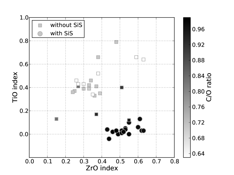
Figure 4: The ZrO and TiO indices for the naked stellar atmospheres in the sample. Squares and circles indicate stars with and without significant SiS absorption with a colorscale that indicates the C/O ratio. Stars for which we have no estimates for $\mathrm{T_{eff}}$, C/O, and [s/Fe] are indicated with open symbols. The figure shows a one-one relation between C/O ratio and presence of SiS absorption in the infrared spectrum.

6 Dust identification

In this section we focus on the 32 stars with significant dust emission features in the IR spectra. We first give an overview of the dust formation sequence in M- and C-type stars and then we compare this with what we find for S-type AGB stars.

6.1 Dust formation in AGB stars

The study of the dust condensation chemistry in AGB stars has mostly focused on the formation of oxygen-rich dust species in M-type stars or carbon-rich dust species in C-stars. In Fig. 5 we show the formation pathways for several dust species that are known to be important in oxygen-rich and/or carbon-rich stellar outflows.

Although it is not yet observationally confirmed, a consistent theory for the dust formation in M-type AGB stars exists. Theoretically, the first condensate to form is alumina grains ($\mathrm{Al_{2}O_{3}}$), which can condense at temperatures as high as 1760 K. When these grains interact with the circumstellar SiO and Ca, melilite is formed. This melilite is first pure gehlenite, but can later on become akermanite due to additional interactions with the circumstellar Mg. Due to the formation of akermanite from gehlenite grains, alumina grains are released from the gehlenite grains and can go on to form additional alumina grains (if the local temperature is above 1510 K) or spinel grains (if the temperature is below 1510 K). The melilite reacts at 1450 K to produce diopside and more spinel. The reaction of diopside and spinel can form anorthite. Further on in the wind, at lower temperatures, these grains can be the seeds for the formation of enstatite, forsterite and the amorphous silicates we observe in many AGB stars. (this scenario was proposed and adapted by Grossman & Larimer, 1974; Onaka et al., 1989; Tielens, 1990; Cami, 2002). Additionally, several species, that are not part of the formation path that eventually ends with silicates, can condense at certain temperatures. For example, due to the reaction of H₂O with Fe, iron oxides form at a temperatue of approximately 900 K, while the magnesium-rich oxides can form at higher temperatures (up to 1200 K) due to the reaction of H₂O with atomic magnesium (Ferrarotti & Gail, 2003).

The broad picture for C-type AGB stars is simpler, but some key details have yet to be filled in. The main dust species detected in carbon-rich stars are amorphous carbon, silicon carbide and magnesium sulfide (Treffers & Cohen, 1974; Goebel & Moseley, 1985; Martin & Rogers, 1987; Andersen et al., 1999; Chan & Kwok, 1990; Hony et al., 2002; Zijlstra et al., 2006; Lagadec et al., 2007; Leisenring et al., 2008). One of the key questions in the carbon-species formation is the importance of mantle chemistry, for example the nucleation of amorphous carbon and magnesium sulfides as mantles around silicon carbide grains have been proposed as important dust formation mechanisms (Lorenz-Martins et al., 2001; Zhukovska & Gail, 2008).

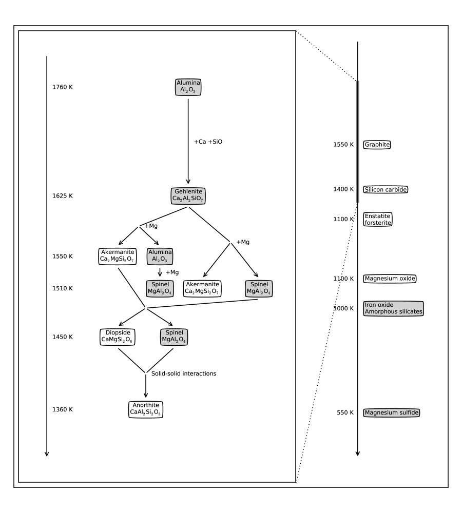
Figure 5: The estimated dust condensation temperatures for different dust species found in AGB stars. The large inset panel zooms in on the dust condensation sequence for oxygen-rich stars, starting from alumina grains. We highlighted the species which were included in our dust decomposition tool in grey.

Assuming a certain dust condensation sequence and an expanding stellar wind, one expects a process called freeze-out, where the sequence is not completed but stops at an intermediate product when the wind density drops below the density required for the next step. This freeze-out has been tentatively observed in AGB stars (e.g. McCabe et al., 1979; Heras & Hony, 2005). An alternative, but qualitatively similar effect could be the exhaustion of oxygen in these S-type environments. If the C/O ratio is close to unity, the formation of alumina grains can use up most of the oxygen atoms available after the formation of CO. If this happens, the density of free oxygen atoms is too low to continue the dust condensation sequence along the path presented in Fig. 5, analogous to the freeze-out (as predicted by Sloan & Price, 1998). We will refer to this process as oxygen depletion.

6.2 Dust decomposition tool

The first crucial step towards understanding the dust condensation sequence of these S-type stars in the present sample is the identification of the dust emission features in the infrared spectra. We developed a simple tool to decompose the infrared spectra into a stellar continuum and the dust emission features of each individual dust species.

If we assume an optically thin circumstellar environment, where the dust condenses out instantaneously once the temperature gets below a certain threshold $T_{0}$ and where the dust grains are in thermal equilibrium, we can write the temperature profile in the circumstellar layers as:

$$T_{\mathrm{dust}}(r)=T_{0}\,\left(\frac{r}{r_{0}}\right)^{-1/2}$$ (1)

where $r_{0}$ corresponds to the radius where the temperature in the outflow drops below $T_{0}$.

The flux coming from a single dust species (using spherical grains and Mie theory) in an optically thin stellar wind with a constant mass-loss rate ${\dot{M}_{\mathrm{d}}}$ and outflow velocity $v$ can be written as:

$$\mathrm{F}_{\nu,\,\mathrm{dust}}=\frac{3\dot{M}_{\mathrm{d}}}{4\,v\,\rho_{d}}\,\frac{Q_{\nu}}{a}\frac{r_{0}}{D^{2}}\int_{1}^{\infty}{B_{\nu}(T_{\mathrm{d}}(x))\,\mathrm{d}x}$$ (2)

where $\rho_{d}$ is the density, $Q_{\nu}$ the absorption efficiency, $a$ the radius of the spherical dust grains, $r_{0}$ the inner radius of the dust shell, $D$ the distance to the object and $T_{\mathrm{d}}(x)$ the temperature profile as in Eq. 1 at a distance $x=r/r_{0}$ (Schutte & Tielens, 1989). Finally, we can combine all constants and unknown parameters into a single parameter $\beta_{i}$ for each dust species $i$. The total spectrum can then be written as:

$$\mathrm{F}_{\nu}=F_{\nu,\,\star}+\sum_{i}\beta_{i}\int_{1}^{\infty}{Q_{\nu,\,i}\,B_{\nu}\,(T_{\mathrm{d}}(x))\,\mathrm{d}x}$$ (3)

where $F_{\nu,\,\star}$ is the flux of the central star at frequency $\nu$ and $\beta_{i}$ is the scaling constant that controls the relative strength of the emission of a specific type of dust.

To arrive at the best fitting model, we use the Lawson and Hanson Non-Negative Least-Squares algorithm (NNLS), which gives the best model under the condition that $\beta_{i}\geq 0$. To estimate the uncertainties on the $\beta_{i}$ parameters, we multiply the uncertainties on the data with a factor until the $\chi^{2}$ value for the best fit is 1. Using these new uncertainties, we add normally distributed noise to the spectrum and calculate the scaling factors $\beta_{i}$ for 1000 randomly disturbed spectra. If the mean value is significantly non-zero (i.e. outside the 99.9% confidence interval), we consider this a positive detection of that dust species in the infrared spectrum.

Because the MARCS model atmospheres still need validation at infrared wavelengths, we prefer to fit the stellar continuum and the emission simultaneously. Therefore, we allow the dust decomposition tool to make any linear combination of the naked stars presented in Sect. 5 and Planck functions of different temperatures, ranging from 500 K to 4000 K, as an estimate for the stellar continuum, $F_{\nu,\,\star}$. The big advantage of using the naked stars is that we can change the relative depth of the CO, SiO, H₂O, and SiS bands to give the optimal fit, while we can change the slope of each individual star with the Planck functions. The drawback, however, is that we will not be able to distinguish between the stellar continuum and additional featureless continuum emission from e.g. metallic iron or amorphous carbon.

Finally, we have to decide which dust species to include in the dust decomposition tool and which to leave out. This is of vital importance because too few dust species will leave us unable to explain some emission features, while too many species would make the interpretation difficult and would lead to degeneracy. We started from a wide range of dust-species, including titanium oxides, titanium carbides, silica and all dust species presented in Fig. 5. We rejected those species that did not improve the goodness-of-fit to the IRS spectrum. The final selection of dust species is:

Amorphous alumina

Amorphous alumina has a high condensation temperature and is thus expected to be at the start of the dust condensation sequence of oxygen-rich stars (see Fig. 5). The most prominent feature of amorphous alumina is at 11.2 $\mu$m with a broad red wing, reaching up to 15.6 $\mu$m. It is a common component of the circumstellar wind of M-type AGB stars. Optical constants have been taken from Begemann et al. (1997).

Amorphous silicates

The strongest emission features due to oxygen-rich dust are the two emission features at 9.8 and 18 $\mu$m due to the stretching and bending of Si-O bonds in amorphous silicates. These features dominate the infrared spectra of most M-type stars. Amorphous silicates form at relatively low temperatures and are thus expected to be at the end of the dust condensation sequence. Here, we have chosen olivines as representative of the typical silicates that are observed in AGB stars. Optical constants have been taken from Jaeger et al. (1994).

Gehlenite

We know from Hony et al. (2009) that the peak of the silicate features in S stars is not at 9.8 $\mu$m as in M-type stars, but shifted towards redder wavelengths, up to 10.6 $\mu$m. Since this cannot be explained with only amorphous silicates, we need to include gehlenite, which is an alumino-silicate (Ca₂Al₂SiO₇). A combination of amorphous silicates, gehlenite and amorphous alumina can explain the broad and shifted 10.6 micron feature. Optical constants have been taken from Mutschke et al. (1998).

19.8 $\mu$m feature

Although the identification of this distinct emission feature at 19.8 $\mu$m is often attributed to iron oxides (Cami, 2002; Posch et al., 2002), other authors have argued that the 19.8 $\mu$m emission, together with additional emission features at 28 and 32 $\mu$m is due to crystalline silicates (Sloan et al., 2003). These features are visible in many M-type stars and most clearly in stars with low mass-loss rates. We were unable to reproduce the 19.8 $\mu$m emission using only crystalline silicates without introducing strong additional emission features in the 9–11 $\mu$m region, which we do not observe. Therefore, we prefer iron oxides (more specifically Mg_0.1Fe_0.9O). Optical constants have been taken from Henning et al. (1995).

The 13 $\mu$m feature

Since the first detection of the 13 $\mu$m feature by Vardya et al. (1986), it has been attributed to different carriers: corundum (crystalline $\mathrm{Al_{2}O_{3}}$, Glaccum, 1995), silica (SiO₂, Speck, 1998) and spinel (MgAl₂O₄, Posch et al., 1999). The debate on the exact carrier of the 13 $\mu$m feature is still ongoing (DePew et al., 2006). In our dust decomposition tool, we tried all three carriers and found that both corundum and spinel can reproduce the emission, but the best results are obtained with spinel. However, detailed modeling is required to attribute the 13 $\mu$m unambiguously to any one carrier, which is beyond the scope of this paper. Optical constants for spinel have been taken from Fabian et al. (2001).

Magnesium sulfides

The most remarkable feature in the spectra of these S-type stars is the broad 26–30 $\mu$m emission feature, attributed to magnesium sulfides. A similar feature has already been observed in two S-type stars, W Aql and $\pi^{1}$ Gru (Hony et al., 2009). Because of the lower spectral resolution of our set of spitzer spectra, the two separate emission peaks at 26 and 28 $\mu$m visible in the ISO/SWS spectra are blended to a single, broad emission feature. In our dust decomposition tool we use the mass absorption coefficients of magnesium sulfide. Optical constants have been taken from Begemann et al. (1994).

Although we could expect the presence of the narrow 11.3 $\mu$m emission feature of amorphous SiC grains (optical constants have been taken from Mutschke et al., 1999) in stars with C/O ratios close to one, replacing one of the aforementioned dust species with amorphous SiC grains resulted in higher $\chi^{2}$ values for all spectra. We can confidently state that amorphous silicates, gehlenite and amorphous alumina are necessary to explain the data. Furthermore, the inclusion of SiC, together with the other dust species, did not significantly lower the $\chi^{2}$ for our sample of S-type stars. Therefore we did not include amorphous SiC grains in the simple fitting routine. More detailed modeling is necessary to make a statement on the absence or presence of SiC grains, but we can conclude that the SiC emission is not strong in any of our stars.

6.3 Overview of the detected dust species

The results of the dust decomposition tool can be found in the online Appendix. Although S-type stars can have C/O ratios very close to unity, the majority of the stars only show dust emission features similar to those found in oxygen-rich stars.

6.3.1 Classification of the dust spectra

Based on the results of the dust decomposition tool, we can subdivide the infrared spectra into 3 groups of spectra with: (i) strong emission features of silicates and gehlenite at 10 and 18 $\mu$m (16 stars), (ii) emission of alumina at 11.2 $\mu$m and of magnesium sulfide at 26–30 $\mu$m (10 stars), or (iii) a 13 $\mu$m and 19.8 $\mu$m emission feature (6 stars).

Group I, stars with strong silicate/gehlenite features:

Approximately half of the stars with dust features in our sample, show a dominant emission feature around 10 $\mu$m, due to the stretching of Si-O bonds of silicate or gehlenite dust grains. In Fig. 6 we show all stars with a strong 10 $\mu$m feature. All spectra in the right panel show substructure at 9.8 and 11 $\mu$m, sometimes accompanied by a sharp peak at 13 $\mu$m, the spectra in the left panel show a single broad emission feature that peaks at wavelengths up to 10.9 $\mu$m. Although the dust decomposition tool can reproduce the emission features with substructure, it is impossible to reproduce the broad and smooth emission features, peaking at 10.5 $\mu$m, visible in the left panel, without showing substructure.

Hony et al. (2009) found 11 stars with a single smooth emission feature at $\sim$ $10.5$ $\mu$m. This feature was only found in S-type AGB stars, while there were no oxygen-rich AGB stars that exhibit the same emission feature. The authors argue that the broad and smooth emission found in these S-type stars is fundamentally different from the substructured emission in oxygen-rich AGB stars and the shift towards longer wavelengths is due to an increase in the magnesium-to-iron ratio in S-type stars.

Group II, stars with alumina, 13 $\mu$m and 20 $\mu$m features:

Fig. 7 shows the six stars in Group II. Although some stars do show some indication for the presence of silicates, the dominant emission features are the 11.2  $\mu$m emission due to amorphous alumina, a strong and sharp 13 $\mu$m feature and the broad 19.8 $\mu$m emission. A similar combination is also common in oxygen-rich stars with low mass-loss rates (Sloan et al., 2003).

Many stars with a strong 13 $\mu$m feature also show the previously detected, unidentified emission features at 28 and 32 $\mu$m indicated with arrows in Fig. 7. Because the 28 and 32 $\mu$m features can blend into a broad plateau with two narrow emission features at 28 and 32 $\mu$m, the dust decomposition tool sometimes wrongly models this broad plateau with emission of magnesium sulfides. This error can easily be identified because the residuals still show the narrow 28 and 32 $\mu$m emission peaks.

Several carriers have been suggested for these features, the most important candidates being crystalline silicates. However, the dust decomposition tool cannot explain the 28 and 32 $\mu$m emission features with these carriers without introducing strong additional emission features that we do not observe.

Group III, stars with magnesium sulfide and alumina

features:

The ten stars in Fig. 8 show two dominant emission features, one attributed to amorphous alumina and the other to magnesium sulfide. Because of the absence of strong silicate features or a strong 19.8 $\mu$m feature, the 26–30 $\mu$m emission of magnesium sulfides is clearly visible on top of the 11.2 $\mu$m of amorphous alumina and can easily be separated from the 28 and 32 $\mu$m emission of Group II stars.

The substructure that can be seen in some of these stars at 6.6 and 13.6 $\mu$m is most likely due to emission of SiS gas near the star, as explained in Sect. 7.2.

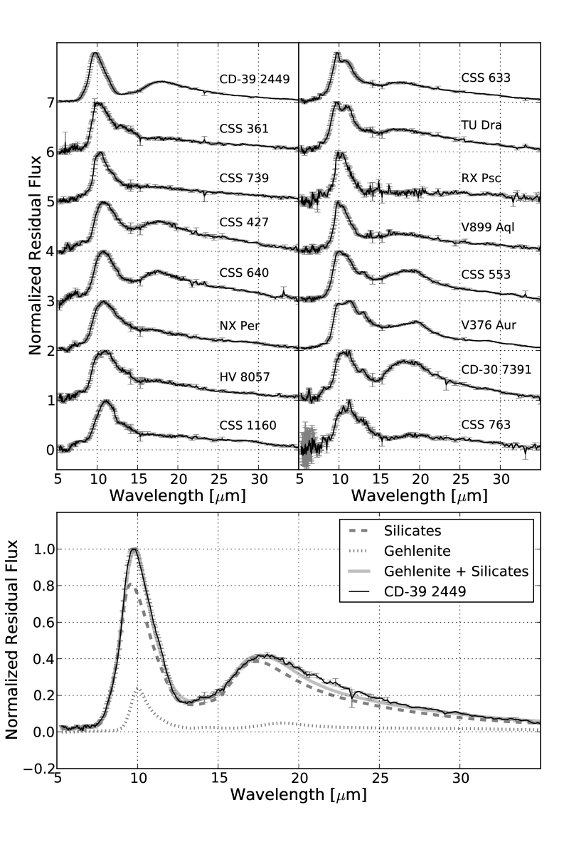
Figure 6: The spectra of all stars in our sample with an infrared spectrum dominated by the 10 and 18 $\mu$m features of silicates and gehlenite (Group I). The top left panel shows the smoothest features at 10 $\mu$m, while the features in the top right panel show substructure at 9.8, 11.2 and/or 13 $\mu$m. The bottom panel shows CD-39~2449, with the relative flux contribution of silicates and gehlenite.

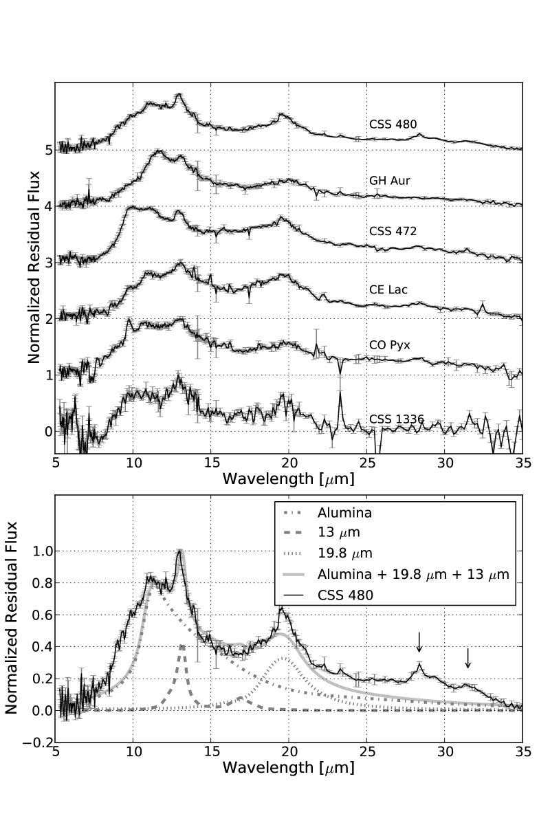
Figure 7: The spectra of all stars in our sample with an infrared spectrum dominated by the emission of amorphous alumina at 11.2 $\mu$m, the 13 $\mu$m and the 19.8 $\mu$m feature (Group II). The bottom panel shows CSS 480, with the relative flux contribution each of these emission features. The previously detected, unidentified emission features at 28 and 32 $\mu$m are indicated with black arrows.

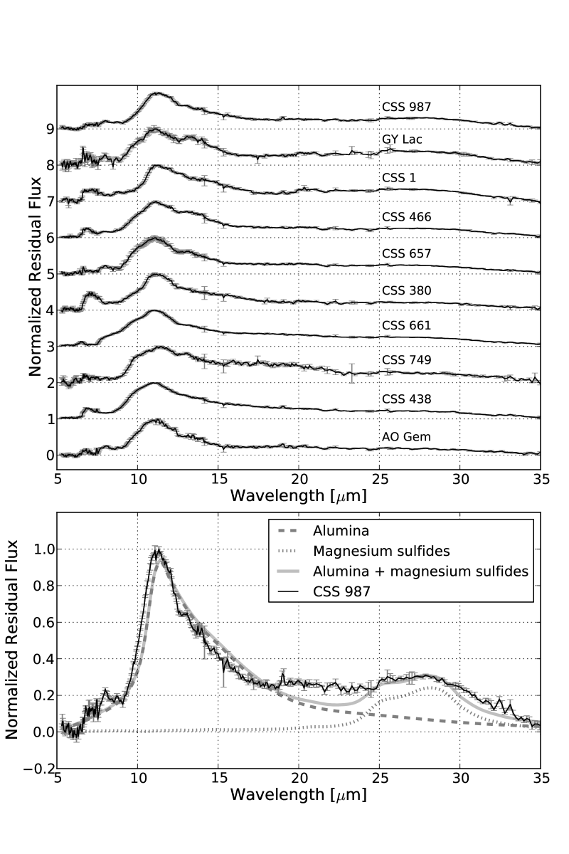
Figure 8: The spectra of all stars in our sample with an infrared spectrum dominated by the emission of amorphous alumina at 11.2 $\mu$m and of magnesium sulfides at 26–30 $\mu$m (Group III). The bottom panel shows CSS 987, with the relative flux contribution of alumina and magnesium sulfides.

6.3.2 C/O dichotomy

In Fig. 9 we show the ZrO and TiO indices of all stars in our sample with dust emission features, using different symbols for the different dust groups. From this figure it is clear that (i) the stars in Group I are distributed more or less uniformly throughout this graph, spanning a wide range of ZrO indices, TiO indices and C/O ratios, while (ii) the stars from Group II are located in the upper left corner of the diagram with low C/O ratios, and (iii) the stars from Group III clutter in the lower right corner with C/O ratios close to unity.

Because the number of stars with known C/O ratios in each separate group is small, we used an unpaired T-test to check whether there is a significant difference in C/O ratios between these groups. We found that the C/O ratios of stars in Group II are significantly lower than the values for Group III stars ($P<0.1\%$). This dichotomy shows that there is a clear dependence of the circumstellar dust mineralogy on the chemical composition of the stellar atmosphere in general and more specifically on the C/O ratio.

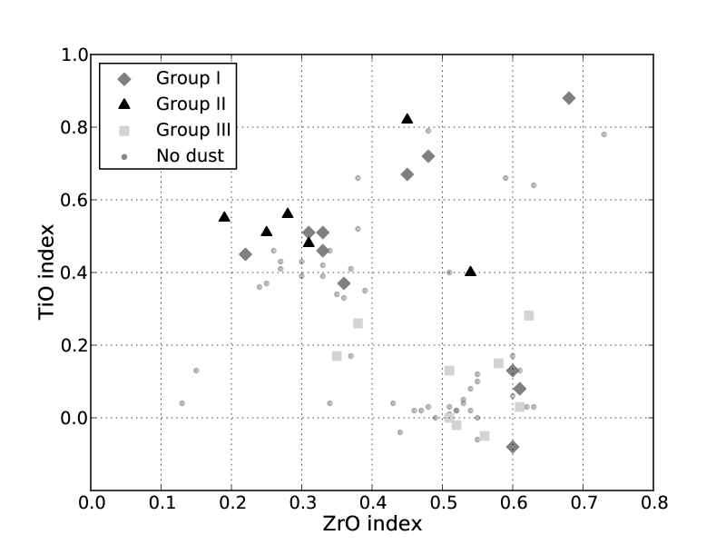
Figure 9: The ZrO and TiO indices for the stars with different types of dust emission features. Group I, II and III are respectively indicated with dark grey diamonds, black triangles and light grey squares. The stars without dust emission features are shown as dots for comparison.

6.3.3 Comparison with the Sloan & Price classification

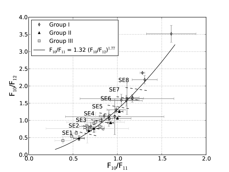
Figure 10: The classification scheme for IR spectra of AGB stars, presented in Sloan & Price (1995, 1998). Group I, II and III are respectively indicated with grey diamonds, black triangles and light grey squares. The solid line shows the powerlaw presented in the original paper. The dashed lines indicate the boundaries between the subsequent classes of the Sloan & Price classification.

Sloan & Price (1995, 1998) also present a classification scheme for IR spectra of AGB stars, using flux ratios at 10, 11, and 12 $\mu$m to quantify the shape of the spectrum in that region. The ratio F₁₀/F₁₁ is an a proxy for the width of the 10 $\mu$m feature and F₁₀/F₁₂ for the strength of the red shoulder. Sloan & Price (1995) find that these flux ratios are strongly correlated and represent this correlation with a powerlaw. Along this sequence, they subdivide the stars into eight separate classes, where the stars with the lowest F₁₀/F₁₁ and F₁₀/F₁₂ ratios fall in the SE1 class and the stars with highest ratios in the SE8 class.

The interpretation of this sequence is that the spectral appearance of the stars in classes SE1–SE3 is dominated by oxides, the stars in classes SE6–SE8 are dominated by amorphous silicates and the intermediate classes show indications of both dust species. This change in spectral appearance with increasing SE-class number has been explained as either an effect of increasing mass-loss rates (for example in Sloan et al., 2003; Pitman et al., 2010) or an effect of decreasing C/O ratio (Sloan & Price, 1998). Both interpretations are based on the fact that alumina grains condense before silicate grains. If the binding of oxygen and alumina uses up the available oxygen, no free atoms will remain to form silicate grains, and alumina grains will dominate the resulting shell (Stencel et al., 1990). The difference between both interpretations is only whether the mass-loss rate or the C/O ratio is the dominating cause of this observed sequence.

In Fig. 10 we compare this power law with the flux ratios we find for the stars in our sample of S-type stars. Although we subtract the continuum flux in a different way, using the continuum estimates determined by the dust decomposition tool, as a combination of naked stellar photospheres and Planck curves of different temperatures, instead of the adapted Engelke function used by Sloan & Price (1998), we find a similar relation between the flux ratios.

The majority of the S-type stars in our sample have classification SE1–SE4, and only a third of the stars have classification SE5–SE8, similar to the findings in Sloan & Price (1995, 1998). Based on our sample, we find that most stars from Group I can be classified as SE5–SE8 stars, while stars from Group II and Group III make up classes SE1–SE4. Although Group II and Group III stars clearly have different IR spectra at longer wavelengths, they have similar 10–12 $\mu$m features and hence there is no difference between the Sloan & Price classification of both groups. Hence, the stars with C/O ratios close to unity (Group III) make up the same IR classes as stars with low C/O ratios (Group II). This is contradictory to the idea that the 10–12 $\mu$m emission is determined by the photospheric C/O ratio for AGB stars. However, there is still a likely difference between the position of these stars in Fig. 10. Most stars of Group III are situated below the powerlaw, while the stars of Group II are above it. If this effect is real, we can conclude that the C/O ratio does not determine the Sloan & Price classification, but might explain the spread on this correlation, while the Sloan & Price class is determined by the mass-loss rate.

7 Molecular emission features

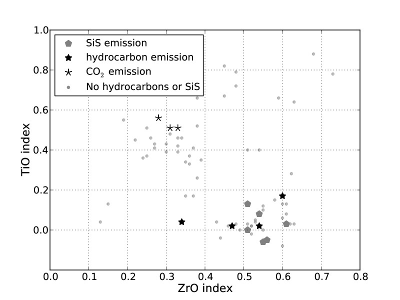
Figure 11: The ZrO and TiO indices for the stars with emission features due to hydrocarbons, SiS or CO₂. The other stars in the sample are shown as dots for comparison.

7.1 Hydrocarbon emission

Hydrocarbon molecules exhibit very characteristic emission features in the 5–14 $\mu$m region, the most prominent at 6.2, 7.9, 8.6, and 11.2 $\mu$m. These features arise from the bending and stretching of the carbon and hydrogen bonds in the large molecules. Peeters et al. (2002) showed that the 7.9 $\mu$m PAH feature can be very different from source to source. They classified the PAH spectra in three classes, based on the peak wavelength of this feature. For type C sources, the peak of this feature is shifted to 8.2 $\mu$m, marking a clear difference with the 7.9 $\mu$m feature of class B PAHs and the 7.6 $\mu$m feature of class A PAHs.

Smolders et al. (2010) present the detection and identification of polycyclic aromatic hydrocarbon (PAH) emission in four S-type AGB stars from the present sample (BZ CMa, KR Cam, CSS 173 and CSS 757). Based on the peak-wavelength, BZ CMa is the only one that shows the B class PAHs resembling PNe, Herbig Ae/Be stars, and red supergiants (Tielens, 2008). The other three stars can be classified as rare class C sources resembling some of the PAHs found in post-AGB stars (Gielen et al., 2009), the carbon-rich red giant HD 100764 (Sloan et al., 2007) and in a disk around the oxygen-rich K giant HD 233517 (Jura et al., 2006).

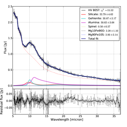
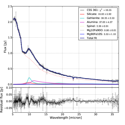
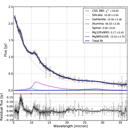
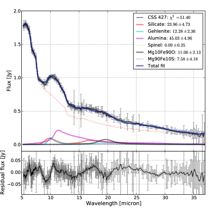
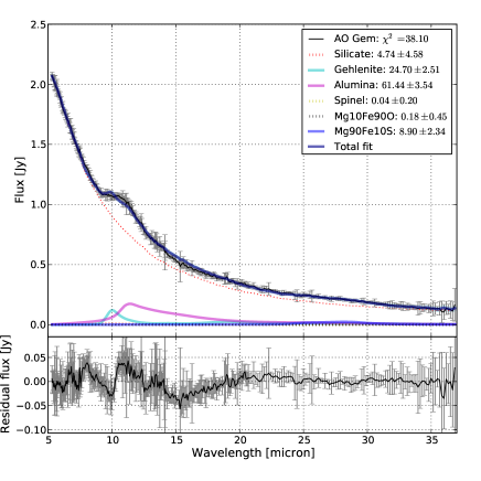
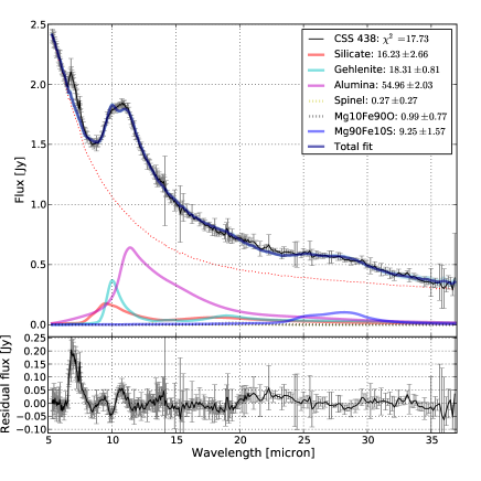
Figure 17: Continued

Furthermore, these relatively red emission features are consistent with the strong correlation found between the centroid wavelength of the 7.9 $\mu$m feature and the temperature of the central star (Sloan et al., 2007; Keller et al., 2008; Acke et al., 2010). The detection of PAHs in four S-type stars extends this correlation towards lower temperatures and more redshifted features. This is consistent with the hypothesis that Class C PAH spectra arise from a mixture of aliphatic and aromatic hydrocarbons, perhaps as isolated PAH molecules embedded in a matrix of aliphatic hydrocarbon bonds, found around stars with weak UV radiation fields (see Pendleton & Allamandola, 2002, Fig. 17). The hydrocarbons around CSS~757, KR~Cam, and CSS~173 thus represent the composition as condensed in the AGB wind, before entering the interstellar medium where harsh UV radiation alters their chemical structure.

In Fig. 11 we again show the ZrO and TiO indices of all stars in our sample. From this figure, it is clear that the stars with hydrocarbon emission have C/O ratios that are higher than average. This is consistent with the idea that in stars with a nearly equal amount of carbon and oxygen atoms, non-equilibrium, shock-driven chemistry can form C₂H₂ molecules in the outer regions of the stellar outflow. These molecules are, further out in the wind, the necessary building blocks for the formation of hydrocarbons (Allamandola et al., 1989).

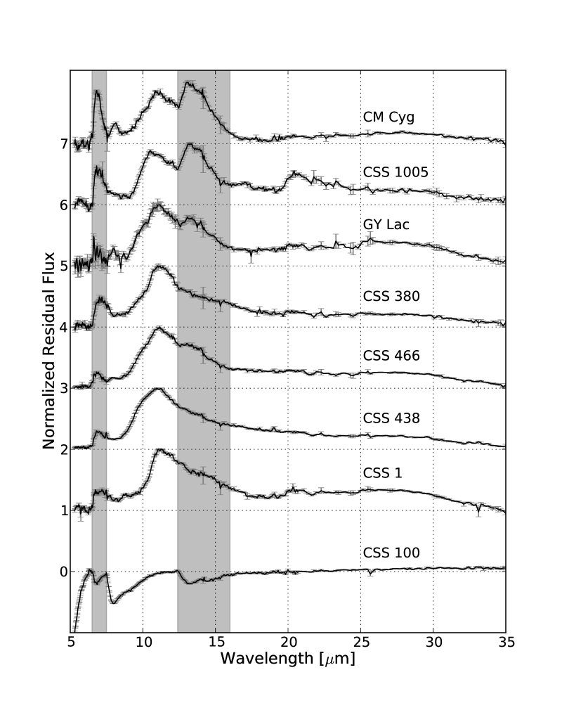
Figure 12: The spectra of all S-type stars in our sample with suspected SiS emission. The grey areas indicate the position of the 6.6 and 13.5 SiS bands. At the bottom, CSS 100, one of the stars with SiS absorption bands, is shown for comparison.

7.2 SiS emission

Sloan et al. (2011) identify the emission features at 6.6 and/or at 13.5 $\mu$m as molecular emission of SiS. These features appear at precisely the wavelengths where they are detected in absorption (Cami et al., 2009). The lack of any wavelength shift strongly suggests that the emission is from SiS in the gas phase. Sloan et al. (2011) only discuss the two stars in our sample with the strongest emission features (CM Cyg and CSS 1005), an additional five stars show a significant emission band at either 6.6 or 13.5 $\mu$m, all of which are classified as Group III stars (see Figs. 12). The presence of these features in emission show that the SiS molecules are not only abundant in the stellar atmosphere, but also in the outer layers of the AGB wind.

In Sect. 5 and 6.3.2 we have shown that both magnesium sulfide grains and SiS molecules are only observed around S-type stars with C/O ratios close to unity (see Fig. 4 and Fig. 9). Therefore, this strong relation between the presence of SiS emission and the dust classification could be explained as a shared dependence on the C/O ratio. However, it is possible that the magnesium sulfide grains in these stars are formed by a reaction of SiS molecules with Mg, as discussed in Sect. 8.4.

7.3 CO₂ emission

The narrow features at 13.9, 15 and/or 16.2 $\mu$m, visible in 9 objects have been identified as CO₂ emission lines (more specifically ¹²C¹⁶O₂). These lines are observed in approximately 30% of oxygen-rich AGB stars, most of which also show a 13 $\mu$m feature (Justtanont et al., 1998; Sloan et al., 2003).

To extract these emission features, we fit a line under the features (at 13.7 and 14.1 $\mu$m for the 13.9 $\mu$m feature, 14.7 and 15.2 $\mu$m for the 15 $\mu$m feature, and 15.9 and 16.5 $\mu$m for the 16.2 $\mu$m feature). As a conservative criterion, we consider a detection of CO₂ emission if all three features are significant at a 99% confidence level. In our sample of S-type stars, we detect significant CO₂ emission features in the 5 objects shown in Fig. 13. The grey bands indicate the location of the emission features.

It is clear from Fig. 11, that all stars with a positive detection of CO₂ emission lines have low C/O ratios. Because CO₂ requires an oxygen-rich environment to form, this dependence on the C/O ratio is not unexpected. Furthermore, although the signal-to-noise ratio and the resolution of the spectroscopic data do not allow for a quantitative analysis of the relationship between the strength of the CO₂ features and the 13 $\mu$m feature, we can confirm that the 13 $\mu$m feature is present in most of the stars with CO₂ emission (4 out of 5 objects). This relation between the presence of the 13 $\mu$m emission and the detection of CO₂ could be explained as a shared dependence on the C/O ratio.

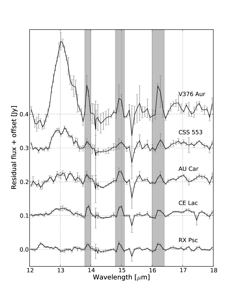
Figure 13: The residual flux, after subtracting a line, of all stars with a positive detection of the CO₂ emission features at 13.9, 15 and/or 16.2 $\mu$m, indicated here with the grey bands.

8 Discussion

8.1 Carbon- versus oxygen-chemistry

We find that almost all S-type AGB stars in our sample show either molecular absorption of molecules such as H₂O or SiO, and/or emission due to dust species such as amorphous alumina or silicates. This mainly oxygen-dominated chemistry in the S-type stars is also confirmed by the stellar parameters, derived from the marcs model atmospheres, where we find that marcs models with C/O ratios between 0.5 and 0.99 can explain the optical spectra of all stars in our sample. This lack of carbon-rich S-type stars is a direct consequence of the spectral classification: for an AGB star to be classified as an S-type star, the ZrO bands need to be present in the optical spectrum. Ferrarotti & Gail (2002) show that the presence of ZrO in the stellar atmosphere critically depends on the C/O ratio of the star. When the C/O ratio becomes larger than unity, the abundance of ZrO in the stellar atmosphere drops several orders of magnitude and hence the strength of the absorption bands drops, until the ZrO bands are not detectable anymore and the star is not classified as an S-type star (Piccirillo, 1980).

However, some stars additionally show absorption bands of SiS, hydrocarbon emission features or the broad emission feature of magnesium sulfide dust, which are typical for carbon-rich sources. However, there are no stars in our sample with an IR spectrum that only shows carbon-rich characteristics. Because all stars in our sample have oxygen-dominated stellar atmospheres, it is remarkable that we can observe emission features that are generally only found in carbon-rich environments. The presence of these emission features indicates the (possibly strong) importance of non-equilibrium chemistry in the circumstellar environment of these AGB stars. The best example of this is the presence of hydrocarbons around KR Cam, CSS 173, CSS 757, and BZ CMa. The thermal equilibrium calculations presented in Ferrarotti & Gail (2002) do not show the production of hydrocarbon molecules, because the majority of the carbon atoms would be locked in the stable and abundant CO molecule. Two main scenarios have been proposed to explain the presence of the hydrocarbon emission in these S-type stars. The first scenario assumes the formation of hydrocarbons from the basic atoms, in the AGB wind itself. Cherchneff (2006) shows that, in AGB stars with a C/O ratio close to unity, non-equilibrium chemistry predicts the formation of C₂H₂ molecules in the stellar outflow (Cherchneff et al., 1992; Cau, 2002), which are the building blocks for hydrocarbons (Allamandola et al., 1989). Although this mechanism can explain the formation of hydrocarbons around S-type stars, C₂H₂ has a very distinct and sharp absorption feature at 13.7 $\mu$m, which is not observed in our S-type stars. The second scenario starts from larger, carbonaceous grains that are broken down into smaller structures, such as hydrocarbons. However, this scenario still requires the presence of carbonaceous dust grains in an oxygen-rich stellar environment.

8.2 Variability characteristics versus dust properties

The stellar winds in AGB stars are commonly attributed to the coupled effect between large amplitude pulsations and radiation pressure on dust grains (Hoefner et al., 1998). This relationship between the pulsations of the stellar atmosphere and the circumstellar environment can be translated into in a relationship between the properties of the infrared spectrum and the variability characteristics of the star. For oxygen-rich stars, a survey of the globular cluster 47 Tuc has shown that not only the mass-loss rate, but also the dust mineralogy changes as the stars evolve towards higher luminosities and longer pulsation periods (Lebzelter et al., 2006; van Loon et al., 2006; McDonald et al., 2011).

We were able to derive the period and amplitude of the pulsations for 55 out of the 87 S-type stars in our sample. This gives us a small subset of stars with and without a dusty circumstellar environment with known variability characteristics. An analysis of this subset shows no significant difference between the periods and amplitudes of the stars with and without dust emission. Apparently for these S-type AGB stars, the period and amplitude of the pulsations are not enough to explain why approximately 65% of the stars have no circumstellar dust, while the other 35% do. Furthermore, it is remarkable that we have detected 5 Mira-like pulsators without significant dust emission features. Looking at the slope of the IR spectra, we can argue that three of these stars have a continuum excess, which might arise from amorphous carbon or metallic iron (AU~Car, RX~Car and CSS~724). However, CSS 794 and XY CMi show no dust excess at all.

Furthermore, a multivariate analysis of the variability characteristics, the stellar parameters and the results from the dust decomposition tool found no significant correlation with either amplitude or period. From this, we can conclude that during this short evolutionary phase where a star is visible as an S-type star, the period and amplitude are not indicative for the mineralogy or the dust mass-loss rate.

8.3 Dust formation around S-type AGB stars

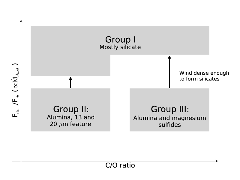
Figure 14: Schematical overview of the proposed idea for dust formation in S-type AGB stars.

In Sect. 6 the dust decomposition tool was used to quantify the contribution of dust emission features to the infrared flux between 5 and 35 $\mu$m. A multivariate analysis of these parameters, together with the stellar parameters ($T_{\mathrm{eff}}$, C/O and [s/Fe]) yields four significant correlations (using a 99% certainty interval) shown in Fig. 15. As an indication for significance of the correlation, we give the probability of obtaining a Pearson, Spearman or Kendall correlation coefficient at least as extreme as the one that was actually observed, assuming that there is no correlation between the two given variables. In order to interpret these p-values correctly, one has to keep in mind that Pearson assumes a linear correlation, while Spearman and Kendall are ranking coefficients. Because we look at ten parameters and thus effectively investigate 45 possible correlations, we have to acknowledge the possibility for a false-positive correlation. All important correlations are shown in Fig. 15.

Silicates and total dust emission

If we remove the outlier V376 Aur, we find a significant correlation between the total dust emission and the flux percentage of silicate features, shown in Fig. 15(a). This correlation indicates that stars with a larger dust excess, and thus a higher dust mass-loss rate, also tend to form silicates in their circumstellar environment. This is in close agreement with the study of Galactic bulge AGB stars (Blommaert et al., 2006) and the study of AGB stars in the Large Magellanic Cloud presented in Dijkstra et al. (2005). Here, the authors find that the dust features displayed by oxygen-rich stars are mainly ascribed to alumina for low dust mass-loss rates, while stars with higher dust mass-loss rates show an increasing amount of silicates. Furthermore, if we look at the total dust excess in the three groups, we find that, on average, Group III stars have a higher dust excess than Group I and Group II stars. Although the difference is only tentative, this is still a noteworthy dichotomy between the three groups, because this is what could be expected based on the results of Blommaert et al. (2006) and Dijkstra et al. (2005).

Silicates and alumina

In Fig. 15(b) we show the significant and strong inverse correlation between the relative flux contribution of alumina and silicates. This correlation can be explained by the standard dust condensation sequence, if we take into account freeze-out. Alumina seeds are formed early on in the dust-condensation sequence at high temperatures, but if the density in the wind is high enough, eventually silicates will form and hence the relative flux contribution of alumina will decrease as the flux contribution of silicates increases.

Magnesium sulfides and alumina

In Fig. 15(c) a strong correlation between the relative flux contribution of magnesium sulfides and alumina is shown. This correlation is unexpected because the presence of alumina grains points to an oxygen-rich circumstellar chemistry while magnesium sulfide emission is usually found in carbon-rich stars. Because this is the first time that this correlation is observed, it can be considered as a new constraint on any dust formation hypothesis for S-type AGB stars.

Magnesium sulfides and silicates

In Fig. 15(d) we show the inverse correlation between the relative flux contribution of silicates and magnesium sulfides. This correlation does not add extra constraints, because it is a consequence of the correlations between the relative flux contribution of (i) silicates and alumina and (ii) magnesium sulfides and alumina.

We propose that the dust formation in S-type stars is critically dependent on the C/O ratio and the total mass-loss rate. Because we expect that silicates only form further out in the wind where the temperature is low enough, the dust condensation sequence can be cut short before silicates start to condense. This could happen because (i) the density in the wind is too low to initiate the necessary chemical reactions (freeze-out) or (ii) there is not enough free oxygen to form the next dust species in the dust condensation sequence (oxygen depletion). At this point, stars with C/O ratios close to unity can only form alumina grains and possibly magnesium sulfide. Stars with lower C/O ratios still have enough free oxygen atoms to form alumina and the carriers of the 13 $\mu$m and 19.8 $\mu$m features. In stars with higher mass-loss rates, the density throughout the wind is high enough to start forming silicates. Because the formation of silicates requires a large number of oxygen atoms, the density at which silicates can condense might depend on the C/O ratio.

This hypothesis can explain perfectly why we can find Group I stars with any C/O ratio, as seen in Fig. 9, while Group II stars are clearly oxygen-rich and Group III stars have C/O ratios close to unity. Furthermore, this hypothesis explains the difference in total dust excess between the groups and it takes into account the tentative correlation between the strength of the silicate emission and the total dust excess.

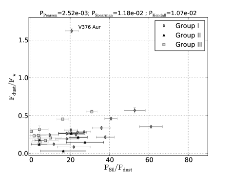
(a) The ratio of the integrated dust emission over the stellar emission versus the relative contribution of silicates to the total dust emission in percentages.

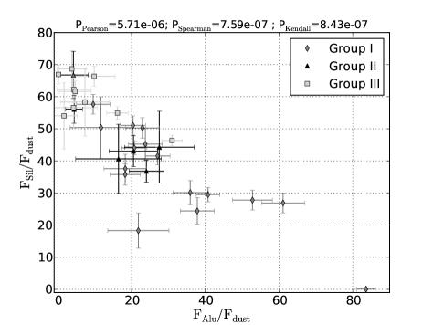
(b) Relative contribution of silicates and alumina to the total dust emission in percentages.

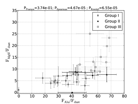
(c) Relative contribution of magnesium sulfides and alumina to the total dust emission in percentages.

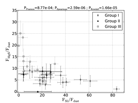
(d) Relative contribution of magnesium sulfides and silicates to the total dust emission in percentages.

Figure 15: All significant correlations presented in Section 8.3. Above each figure, you can find the Spearman, Kendall and Pearson probabilities of each of the correlations. Please keep in mind that Pearson can only be used for linear relationships, while Spearman and Kendall are both rank-test and thus can be used for any relation between two parameters. The correlations in figures 15(b), 15(c) and 15(d) are clearly significant, while the correlations in figure 15(a) is only tentative.

8.4 The formation of magnesium sulfides in S-type AGB stars

A number of observational and theoretical studies on the 26–30 $\mu$m emission feature in AGB and post-AGB stars, and in the environment of planetary nebulae show that magnesium sulfide is a wide-spread dust component in carbon-rich evolved stars (Hony et al., 2002; Volk et al., 2002; Zijlstra et al., 2006; Lagadec et al., 2007). As magnesium sulfide is usually observed in circumstellar environments dominated by carbon chemistry, the chemical models have focused on magnesium sulfide formation in a carbon-rich environment with and without silicon carbide condensation (Zhukovska & Gail, 2008). There are two main pathways to form magnesium sulfide grains. If the sulfur is locked in SiS molecules, the necessary reaction is:

$$\mathrm{Reaction\ I:\ }\mathrm{SiS}+\mathrm{Mg}\rightarrow\mathrm{MgS\ (solid)}+\mathrm{Si}$$

If the sulfur is free from the SiS molecules because, for example, the silicon is consumed in the formation of silicon carbide, the free sulfur forms H₂S molecules and the main reaction is:

$$\mathrm{Reaction\ II:\ }\mathrm{H_{2}S}+\mathrm{Mg}\rightarrow\mathrm{MgS\ (solid)}+\mathrm{H_{2}}$$

Zhukovska & Gail (2008) find for carbon-rich AGB stars that only the growth of magnesium sulfide as mantles on SiC cores, following reaction II, can produce enough magnesium sulfide dust to explain the observations. Hence, following this formation mechanism, the production of magnesium sulfide depends on silicon carbide grains (i) to free the sulfur from SiS molecules (so that H₂S can be formed) and (ii) as core grains on which the magnesium sulfide can form a mantle. Since we do not see strong silicon carbide emission features in any of our stars (although we cannot completely rule out the presence of a weak emission feature in the 10–12 $\mu$m range) we conclude that alternative seeds are necessary.

If reaction II is the dominant formation path to form magnesium sulfides, we need to free the sulfur from SiS before this reaction can take place. In a mixed chemistry region, there is a much wider variety of silicon-rich dust species as compared to a purely carbon-rich chemistry (see Fig. 5). Already at relatively high temperatures the corundum reacts with circumstellar gas to form gehlenite and further interactions lead to other silicon-bearing dust grains such as akermanite, diopside, anorthite, and eventually silicate grains. All these dust species can consume silicon, hence allowing the free sulfur to form the H₂S molecules, necessary for reaction II.

Although these silicon-bearing grains have emission peaks in the 10–20 $\mu$m range, the infrared spectra of most of the stars with clear magnesium sulfides emission also show amorphous alumina, without clear observational evidence for any silicon-bearing dust species. Hence, the observations indicate that the presence of silicates or other silicon-bearing dust species is not a strict requirement for the formation of magnesium sulfides.

Because many stars with magnesium sulfide emission show additional emission peaks at 6.6 and 13.5 $\mu$m, due to molecular emission of SiS, the observations seem to indicate that reaction I is the main formation mechanism in these S-type AGB stars. Because sulfur is less abundant than magnesium, we can expect that more influx of SiS molecules in the wind would lead to more magnesium sulfides being formed. Furthermore, because SiS molecules are only formed in S-type stars with C/O ratios larger than 0.96, it automatically follows that we will only detect magnesium sulfide dust in stars with similar high C/O ratios, as is shown in Fig. 9.

According to Zhukovska & Gail (2008), the formation path of magnesium sulfide is more efficient as heterogeneous growth on a different type of dust particles that already have moderate radii. The dust species that may serve as carrier grains need to form dust grains with a size not much smaller than about 0.1 $\mu$m and need to be formed early on in the wind. The correlation shown in Fig. 15(c) indicates an (indirect) relation between alumina grains and the magnesium sulfide formation. Because alumina can form very early on in the wind (at temperatures above 1700 K) and because of the correlation between the relative flux contribution of alumina and magnesium sulfides (see Sect. 8.3), we propose the hypothesis that magnesium sulfides in S-type AGB stars are formed on amorphous alumina grains. In addition, this formation mechanism can explain the presence of SiS emission bands at 6.6 and/or 13.5 $\mu$m in many Group III stars, because it is a key ingredient for the formation of magnesium sulfides.

9 Results and conclusions

We present a new sample of Spitzer-IRS spectra for 87 galactic S-type AGB stars which were selected based on the presence of a ZrO absorption band at optical wavelengths, pulsation characteristics and K-band magnitude. Although the sample is slightly biased towards lower mass-loss rates, we show that we exclude less than 5% of the stars with high mass-loss rates. In addition to the IR spectra, we obtained optical spectra (low and/or high resolution) and infrared photometry for the stars in our sample.

We derived the chemical parameters (T_eff, C/O, [s/Fe] and [Fe/H]) for a large subset of the sample, by comparing the available optical spectra to marcs model atmospheres.

For a large subset of the sample, we provide pulsation characteristics, based on the ASAS, NSVS and AAVSO light curves. The sample contains 6 irregular pulsators, 38 semi-regular variables and 21 Miras. It is remarkable that 5 of the 17 Miras do not show any dust emission features. This does not imply that these stars have no dusty wind, because we cannot exclude the presence of dust species, such as metallic iron and amorphous carbon.

We find that the presence of the SiS absorption band in the S-type stars without dust emission features is critically dependent on the C/O ratio. Stars with C/O ratios lower than 0.96 do not show significant absorption at 6.6 or 13.5 $\mu$m while all naked stellar atmospheres with C/O ratios above 0.96 show significant absorption bands. This opens up the possibility to use the SiS absorption band as an indicator for the C/O ratio.

We present a positive detection and identification of PAH emission in 4 S-type AGB stars, a detailed description and discussion is given by Smolders et al. (2010).

We use a simple tool to decompose the IR spectra of the dust-rich stars. This tool is used to identify the dust species that are visible in the IR spectra and to quantify the relative flux contribution of each dust type to the total flux. Based on this dust decomposition tool, we are able to classify the IR spectra into three distinct groups: (i) stars with strong silicate/gehlenite features, (ii) stars with strong 13 $\mu$m and 20 $\mu$m emission features and (iii) stars with magnesium sulfides and amorphous alumina. The fact that we find three separate classes is already a remarkable result, for example, no star has both a 13 $\mu$m feature and magnesium sulfide emission.

We also find a strong relation between the C/O ratio and mineralogy. We propose that, for stars with low mass-loss rates, the dust-condensation sequence is cut short and the remaining amount of free oxygen, together with the presence of SiS molecules in the wind determines whether sulfides will be formed (Group III) or whether we will observe a 13 $\mu$m and 20 $\mu$m feature (Group II). Stars with higher mass-loss rates can complete the dust formation sequence and form silicate grains (Group I). This scenario is consistent with the correlations shown in Fig. 15.

Finally, we propose the hypothesis that magnesium sulfides in S-type stars are formed by a reaction of SiS molecules with Mg. This is based (i) on the observation that magnesium sulfides are only observed in stars with C/O ratios close to one, where SiS molecules are formed and (ii) on the detection of SiS emission in half of the stars with magnesium sulfide emission, indicating that the SiS molecules are present in the circumstellar environment. Furthermore, based on the formation mechanism of magnesium sulfides in carbon-rich AGB stars, we propose that magnesium sulfide is formed as mantles around dust grains, for example amorphous alumina.

Table 2: The basic data for the stars in our sample. From left to right we find the CSS number, the most frequently used names, the V magnitude (if possible we used an interpolation of the lightcurve at the time of the SAAO JHKL observations), the new JHKL magnitudes, the ZrO and TiO indices and the available optical data.

CSS	name	Vmag	SAAO J	SAAO H	SAAO K	SAAO L	ITiO	IZrO	Optical Spectra
1	CSS 1
32	RX Psc	12.08	6.31	5.33	5.02	4.62			Hermes
38	CSS 38								Hermes
91	NX Per
100	CSS 100
127	CSS 127	12.99	6.30	5.18	4.84	4.50	0.29	0.45	SAAO, WHT, Hermes
166	CSS 166	13.40	6.83	5.64	5.27	4.93	0.26	0.46	SAAO, WHT
173	CSS 173	11.15	6.69	5.55	5.29	4.94	0.21	0.27	SAAO, WHT, Hermes
177	KR Cam						0.26	0.44	WHT, Hermes
179	CSS 179						0.24	0.52
191	GH Aur		5.72	4.49	4.08	3.67	0.43	0.40	WHT, Hermes
196	V376 Aur						0.57	0.16	WHT, Hermes
202	CD-39 2449						0.41	0.23	SAAO
218	NP Aur						0.92	0.37	WHT, Hermes
220	CF Gem	13.56	6.64	5.37	4.97	4.60	0.22	0.43	WHT, Hermes
229	HV 8057	13.77	6.22	5.17	4.76	4.24	0.88	0.29	SAAO
267	CSS 267	14.09	6.64	5.37	4.97	4.60	0.36	0.46	SAAO, WHT
281	BZ CMa	12.77	6.59	5.38	4.96	4.47	0.20	0.38	SAAO, Hermes
282	CSS 282	13.79	6.99	5.68	5.25	4.80	0.30	0.52	SAAO, WHT
298	CSS 298	11.53	6.87	5.77	5.48	5.23			SAAO, WHT, Hermes
300	CPD-19 1672	9.90	6.31	5.34	5.14	4.97	0.22	0.13	SAAO, Coralie, Hermes
315	CD-43 2976	11.31	6.41	5.41	5.13	4.94	0.46	0.16	SAAO, Coralie
325	XY CMi	14.51	6.79	5.74	5.37	4.97	0.55	0.15	SAAO, WHT, Hermes
328	CD-30 4223	10.38	6.62	5.65	5.44	5.21	0.26	0.30	SAAO, Coralie
352	CSS 352	12.98	6.89	5.70	5.35	4.96	0.43	0.29	SAAO, Hermes
361	CSS 361	12.58	6.21	5.08	4.75	4.39	0.30	0.50	SAAO
371	CSS 371	12.73	7.01	5.75	5.36	4.95	0.28	0.44	SAAO, Hermes
380	CSS 380	14.92	6.96	5.70	5.16	4.51	0.23	0.46	SAAO
393	CSS 393	11.69	6.88	5.79	5.44	5.12	0.22	0.34	SAAO, Coralie
417	CSS 417	13.14	6.67	5.42	5.01	4.62	0.16	0.37	SAAO, Hermes
427	CSS 427		6.85	5.49	4.98	4.63	0.30	0.53	SAAO
431	AO Gem						0.23	0.48	WHT, Hermes
438	CSS 438		7.00	6.00	5.48	4.89	0.27	0.50	SAAO
443	EX Pup		7.11	6.15	5.71	5.27	0.90	0.20	SAAO
453	CSS 453	12.27	6.35	5.17	4.80	4.53	0.40	0.15	SAAO
454	CSS 454	10.62	6.25	5.28	5.02	4.78	0.39	0.26	SAAO, WHT, Coralie, Hermes
457	CSS 457	11.07	6.56	5.54	5.26	5.10	0.46	0.14	SAAO
466	CSS 466		6.84	5.27	4.60	3.88	0.33	0.35	SAAO
472	CSS 472	12.94	6.60	5.44	5.10	4.92	0.57	0.05	SAAO
478	CSS 478	11.20	6.55	5.44	5.15	4.97	0.39	0.13	SAAO, Coralie
480	CSS 480	11.43	5.93	4.88	4.56	4.34	0.54	0.08	SAAO, Coralie
489	CD-29 5912	10.59	6.34	5.34	5.08	4.83	0.37	0.25	SAAO, Coralie
528	CSS 528	12.34	6.60	5.50	5.17	4.92	0.44	0.13	SAAO
531	CSS 531		7.11	5.83	5.40	5.09	0.48	0.37	SAAO
545	CO Pyx	15.00	6.73	5.82	5.40	4.88	0.81	0.10	SAAO, Hermes
553	CSS 553	12.70	6.13	4.93	4.56	4.34	0.56	0.13	SAAO
558	CSS 558	12.65	6.62	5.54	5.21	4.94	0.45	0.23	SAAO
584	CSS 584	13.00	6.49	5.23	4.82	4.45	0.20	0.40
598	CSS 598	13.41	6.85	5.69	5.36	5.07	0.34	0.54	SAAO
603	CD-30 7391	10.67	5.90	4.87	4.60	4.46	0.48	0.10	SAAO, Coralie
604	CSS 604	14.26	7.20	5.98	5.60	5.31	0.32	0.53	SAAO
613	CSS 613	13.19	6.38	5.07	4.67	4.29	0.23	0.44	SAAO
622	CSS 622	13.35	6.67	5.39	4.95	4.51	0.24	0.39	SAAO
633	CSS 633		6.97	5.85	5.29	4.55	0.74	0.32	SAAO
635	CSS 635	12.61	6.97	5.77	5.42	5.04	0.18	0.42	SAAO
640	CSS 640	13.68	6.96	5.70	5.34	5.05	0.33	0.52	SAAO
650	CSS 650	10.98	6.40	5.36	5.07	4.95	0.41	0.20	SAAO
657	CSS 657	12.46	6.78	5.51	4.99	4.33	0.26	0.46	SAAO
661	CSS 661	12.76	6.49	5.15	4.63	4.05	0.25	0.19	SAAO
665	CSS 665	13.22	6.91	5.79	5.47	5.26	0.28	0.51	SAAO
679	AU Car		5.89	4.73	4.27	3.88			SAAO
682	CSS 682	11.71	6.19	5.07	4.74	4.45	0.44	0.18	SAAO
690	RX Car		6.54	5.42	4.90	4.39	0.80	0.26	SAAO
718	CSS 718	12.18	6.36	5.25	4.93	4.66	0.43	0.15	SAAO
719	CSS 719	12.27	6.53	5.34	4.99	4.64	0.25	0.44	SAAO
723	CSS 723	13.41	7.09	5.95	5.40	4.94	0.07	0.04	SAAO
724	CSS 724	13.07	6.20	5.19	4.83	4.46			SAAO
739	CSS 739	13.35	6.81	5.95	5.50	4.81	0.80	0.21	SAAO
749	CSS 749	13.49	6.52	5.21	4.80	4.36	0.33	0.46	SAAO
757	CSS 757	13.08	6.68	5.37	4.93	4.54	0.20	0.45	SAAO
763	CSS 763	12.48	6.67	5.40	5.03	4.67	0.47	0.16	SAAO
783	CSS 783	11.16	6.66	5.65	5.36	5.15	0.39	0.12	SAAO
794	CSS 794		6.88	5.70	5.26	4.86	0.79	0.73	SAAO
806	CSS 806	14.68	7.31	5.70	5.13	4.75	0.31	0.11	SAAO
881	CSS 881	12.88	6.47	5.09	4.62	4.26	0.27	0.37	SAAO
921	CSS 921	12.01	5.99	4.88	4.54	4.32	0.46	0.10	SAAO
987	CSS 987		7.68	6.19	5.57	5.00	1.13	1.13	SAAO
1005	CSS 1005	13.30	6.26	5.05	4.62	4.14	0.22	0.47	SAAO
1046	CSS 1046		6.40	5.27	4.92	4.58			WHT
1077	CSS 1077	11.61	6.40	5.37	5.07	4.83	0.46	0.18	SAAO, WHT
1087	TU Dra								WHT
1137	V734 Cyg						0.61	0.32	WHT
1138	CSS 1138								WHT
1160	CSS 1160	11.69	7.03	5.99	5.49	4.79			WHT
1180	CM Cyg						0.29	0.49	WHT
1181	V899 Aql		7.00	6.07	5.56	4.90	1.29	3.88	WHT
1305	CE Lac						0.62	0.12	WHT
1307	GY Lac						0.22	0.48	WHT
1311	BD+02 4571	9.15	6.42	5.60	5.42	5.19	0.07	0.05	WHT, Hermes
1336	CSS 1336						0.50	0.16	WHT

Table 2: continued.

Table 3: The results of the period analysis for all stars as described in Section 4.2. A dash indicates that there was no significant pulsation period found or that the timeseries did not cover a timespan longer than the found period.

name	Type	Period	Type (GCVS)	Period (GCVS)	name	Type	Period	Type (GCVS)	Period (GCVS)
		days		days			days		days
CSS 1		-	-	-	CSS 553		-	-	-
RX Psc	Mira	281	Mira	281	CSS 558	SR	142	-	-
CSS 38		-	-	-	CSS 584	SR	301	-	-
NX Per		-	Mira	-	CSS 598	Irr	-	-	-
CSS 100		-	-	-	CD-30 7391		-	-	-
CSS 127	SR	239	-	-	CSS 604		-	-	-
CSS 166	SR	262	-	-	CSS 613	SR	127	-	-
CSS 173	SR	139	-	-	CSS 622	SR	159	-	-
KR Cam		-	SR	-	CSS 633		-	-	-
CSS 179		-	-	-	CSS 635	SR	150	-	-
GH Aur		-	Mira	388	CSS 640	SR	125	-	-
V376 Aur		-		-	CSS 650	SR	102	-	-
CD-39 2449	SR	167	-	-	CSS 657	Mira	409	-	-
NP Aur		-	Mira	334	CSS 661	Mira	409	Mira	418
CF Gem	SR	153		-	CSS 665	SR	110	-	-
HV 8057	Mira	370	Mira	370	AU Car	Mira	347	Mira	332
CSS 267	Irr	-	-	-	CSS 682	Irr	-	-	-
BZ CMa	Mira	333	Mira	320	RX Car	Mira	336	Mira	333
CSS 282	Irr	-	-	-	CSS 719	SR	278	-	-
CSS 298	SR	142	-	-	CSS 723	SR	223	-	-
CD-43 2976	SR	74	-	-	CSS 724	Mira	281	Mira	280
XY CMi	Mira	271		-	CSS 739	Mira	336	-	-
CD-30 4223	SR	198	-	-	CSS 749	SR	148	-	-
CSS 352	SR	115	-	-	CSS 757		-	-	-
CSS 361	SR	125	-	-	CSS 763	SR	83	-	-
CSS 371	SR	146	-	-	CSS 783	Irr	-	-	-
CSS 380	Mira	363	-	-	CSS 794	Mira	307	Mira	305
CSS 393	SR	92	-	-	CSS 806		-	-	-
CSS 417	SR	167	-	-	CSS 881	SR	158	-	-
CSS 427		-	-	-	CSS 921	Irr	-	-	-
AO Gem		-	Mira	313	CSS 987	SR	286	-	-
CSS 438	Mira	405	-	-	CSS 1005		-	-	-
EX Pup	SR	290	Mira	289	CSS 1046		-	-	-
CSS 453	SR	61	-	-	CSS 1077	SR	70	-	-
CSS 454	SR	79	-	-	TU Dra		-	Mira	345
CSS 457	SR	69	-	-	V734 Cyg		-	Mira	310
CSS 466	Mira	385	-	-	CSS 1138		-	-	-
CSS 472	SR	95	-	-	CSS 1160	Mira	357	Mira	360
CSS 478	SR	62	-	-	CM Cyg		-	Mira	255
CSS 480	SR	117	-	-	V899 Aql	Mira	374	SR	100
CD-29 5912	SR	103	-	-	CE Lac		-	SR	107
CSS 528	SR	107	-	-	GY Lac		-	Mira	-
CSS 531		-	-	-	CSS 1336		-	-	-
CO Pyx	Mira	329	Mira	-				-	-

Table 4: Effective temperature, C/O ratio and gross s-process overabundance of S stars. Hen 4-NNN lists S stars as in the Simbad database from an unpublished list of Henize (see e.g. Van Eck et al. 2000).The “uncertain” label in the comment column means that the convergence to the quoted set of physical parameters was not as consistent as in all the other cases.

CSS	${\rm T}_{\rm eff}$	C/O	[s/Fe]	Comments
127	3300 $\pm$ 100	0.95 $\pm$ 0.025	1.5 $\pm$ 0.5
166	3300 $\pm$ 100	0.98 $\pm$ 0.010	1.7 $\pm$ 0.3
173	3600 $\pm$ 100	0.97 $\pm$ 0.020	1.5 $\pm$ 0.5	uncertain
177	3350 $\pm$ 150	0.96 $\pm$ 0.010	1.0 $\pm$ 0.5	KR Cam
179	3250 $\pm$ 50	0.98 $\pm$ 0.010	1.5 $\pm$ 0.5
191	3200 $\pm$ 100	0.84 $\pm$ 0.088	1.5 $\pm$ 0.5	GH Aur ; Hα emission ; Mira ; uncertain
196	3250 $\pm$ 50	0.84 $\pm$ 0.088	0.5 $\pm$ 0.5	V376 Aur
202	3500 $\pm$ 100	0.70 $\pm$ 0.200	1.0 $\pm$ 0.3	CD-39 2449 ; Hen 4-8 ;
220	3300 $\pm$ 100	0.98 $\pm$ 0.010	1.5 $\pm$ 0.5	CF Gem
267	3350 $\pm$ 50	0.99 $\pm$ 0.010	1.5 $\pm$ 0.5
281	3300 $\pm$ 100	0.99 $\pm$ 0.010	1.0 $\pm$ 0.5	BZ CMa
282	3300 $\pm$ 100	0.97 $\pm$ 0.020	1.5 $\pm$ 0.5
315	3450 $\pm$ 50	0.63 $\pm$ 0.125	0.6 $\pm$ 0.4	CD-43 2976
325	3200 $\pm$ 100	0.71 $\pm$ 0.210	0.5 $\pm$ 0.5	XY CMi
328	3450 $\pm$ 150	0.93 $\pm$ 0.025	1.0 $\pm$ 0.3	CD-30 4223 ; Hen 4-19 ;
352	3400 $\pm$ 100	0.70 $\pm$ 0.200	1.3 $\pm$ 0.3
361	3300 $\pm$ 100	0.97 $\pm$ 0.020	1.5 $\pm$ 0.5	Hen 4-23
371	3400 $\pm$ 100	0.98 $\pm$ 0.010	1.5 $\pm$ 0.5	Hen 4-26 ; uncertain
380	3150 $\pm$ 250	0.98 $\pm$ 0.010	1.0 $\pm$ 0.7	Hen 4-27 ; Hα emission
393	3450 $\pm$ 50	0.97 $\pm$ 0.020	1.5 $\pm$ 0.5	Hen 4-29
417	3450 $\pm$ 50	0.98 $\pm$ 0.010	1.5 $\pm$ 0.5	Hα emission
427	3200 $\pm$ 100	0.97 $\pm$ 0.020	1.5 $\pm$ 0.5
431	3300 $\pm$ 100	0.96 $\pm$ 0.010	1.5 $\pm$ 0.5	AO Gem ; Hα emission
438	3150 $\pm$ 150	0.96 $\pm$ 0.010	1.5 $\pm$ 0.5
443	2900 $\pm$ 200	0.71 $\pm$ 0.210	0.5 $\pm$ 0.5	EX Pup ; Hα emission
453	3400 $\pm$ 100	0.70 $\pm$ 0.200	0.5 $\pm$ 0.5
454	3400 $\pm$ 100	0.71 $\pm$ 0.210	1.0 $\pm$ 0.2
457	3450 $\pm$ 50	0.63 $\pm$ 0.125	0.5 $\pm$ 0.5	Hen 4-38 ; uncertain
472	3350 $\pm$ 50	0.63 $\pm$ 0.125	0.1 $\pm$ 0.1	MS star
478	3400 $\pm$ 100	0.71 $\pm$ 0.210	0.5 $\pm$ 0.5
480	3350 $\pm$ 50	0.63 $\pm$ 0.125	0.4 $\pm$ 0.3
489	3450 $\pm$ 50	0.63 $\pm$ 0.125	1.0 $\pm$ 0.3	CD-29 5912 ; Hen 4-44
528	3450 $\pm$ 50	0.83 $\pm$ 0.075	0.4 $\pm$ 0.4
531	3250 $\pm$ 50	0.91 $\pm$ 0.012	1.2 $\pm$ 0.2
553	3300 $\pm$ 100	0.70 $\pm$ 0.200	0.4 $\pm$ 0.3
558	3300 $\pm$ 100	0.71 $\pm$ 0.213	0.9 $\pm$ 0.3	Hα emission
584	3300 $\pm$ 100	0.99 $\pm$ 0.010	1.5 $\pm$ 0.5	Hen 4-62 ; uncertain
598	3250 $\pm$ 150	0.97 $\pm$ 0.010	1.5 $\pm$ 0.5
603	3400 $\pm$ 100	0.70 $\pm$ 0.200	0.4 $\pm$ 0.4	CD-30 7391
604	3300 $\pm$ 100	0.98 $\pm$ 0.010	1.5 $\pm$ 0.5
613	3450 $\pm$ 50	0.98 $\pm$ 0.010	1.7 $\pm$ 0.3
622	3200 $\pm$ 100	0.99 $\pm$ 0.010	0.5 $\pm$ 0.4
633	3300 $\pm$ 50	0.91 $\pm$ 0.012	0.2 $\pm$ 0.1	Hen 4-73 ; uncertain
635	3400 $\pm$ 100	0.98 $\pm$ 0.010	1.5 $\pm$ 0.5	Hα emission
640	3250 $\pm$ 50	0.97 $\pm$ 0.010	1.0 $\pm$ 0.3	Hen 4-75
650	3450 $\pm$ 50	0.70 $\pm$ 0.200	0.8 $\pm$ 0.5	Hen 4-77
657	3300 $\pm$ 100	0.97 $\pm$ 0.010	1.5 $\pm$ 0.5	Hen 4-81 ; Hα emission
665	3300 $\pm$ 100	0.97 $\pm$ 0.020	1.5 $\pm$ 0.5
682	3400 $\pm$ 100	0.71 $\pm$ 0.210	0.8 $\pm$ 0.3	Hen 4-92
690	3150 $\pm$ 150	0.71 $\pm$ 0.210	0.3 $\pm$ 0.3	RX Car ; Hα emission ; Mira ; uncertain
718	3300 $\pm$ 100	0.71 $\pm$ 0.213	0.5 $\pm$ 0.5	Hen 4-106 ; uncertain
719	3400 $\pm$ 100	0.99 $\pm$ 0.010	1.5 $\pm$ 0.5
739	3200 $\pm$ 100	0.91 $\pm$ 0.012	0.1 $\pm$ 0.1	Mira
757	3300 $\pm$ 100	0.98 $\pm$ 0.010	1.5 $\pm$ 0.5
763	3300 $\pm$ 100	0.71 $\pm$ 0.213	0.5 $\pm$ 0.5
783	3450 $\pm$ 150	0.71 $\pm$ 0.210	0.5 $\pm$ 0.5
794	3150 $\pm$ 150	0.96 $\pm$ 0.010	0.5 $\pm$ 0.5	Hen 4-122
806	3650 $\pm$ 50	0.83 $\pm$ 0.075	0.5 $\pm$ 0.5	high extinction; uncertain
881	3250 $\pm$ 150	0.99 $\pm$ 0.010	1.0 $\pm$ 0.5
921	3350 $\pm$ 50	0.63 $\pm$ 0.125	0.3 $\pm$ 0.3
1005	3350 $\pm$ 150	0.97 $\pm$ 0.020	1.5 $\pm$ 0.5
1180	3300 $\pm$ 100	0.99 $\pm$ 0.010	1.0 $\pm$ 0.3	CM Cyg ; strong Hα emission
1305	3250 $\pm$ 150	0.70 $\pm$ 0.200	0.3 $\pm$ 0.3	CE Lac
1336	3300 $\pm$ 100	0.63 $\pm$ 0.125	0.4 $\pm$ 0.3

Appendix A Results of the dust decomposition tool

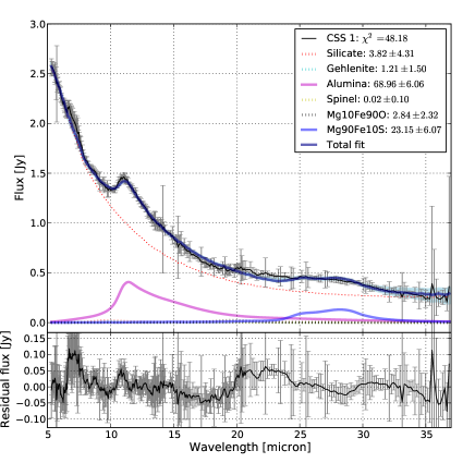
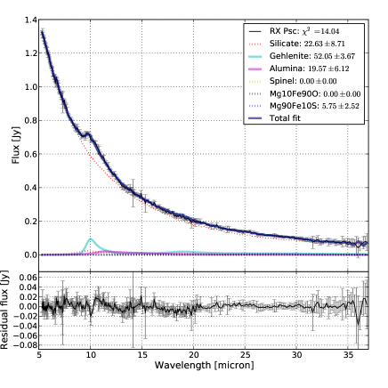
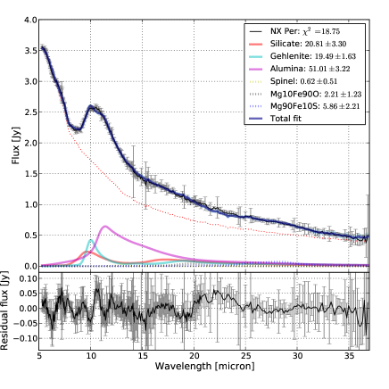
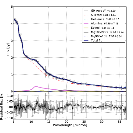
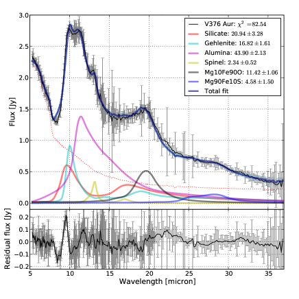
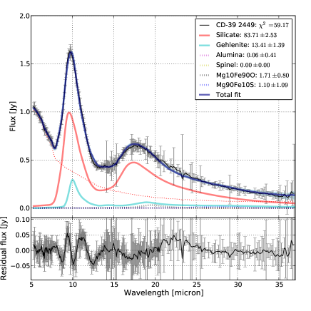
Figure 16: The results of the dust decomposition tool for all stars with dust features. Top panel: the black line shows the Spitzer spectrum, the red dotted line the fit the underlying estimate for the stellar continuum, as derived from the dust decomposition tool and the solid, dark blue line indicates the total fit to the spectrum. Solid lines shown in the legend indicate significant contributions to the spectrum, the dotted lines the non-significant contributions. Bottom panel: the residuals after subtracting the total fit.

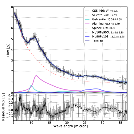
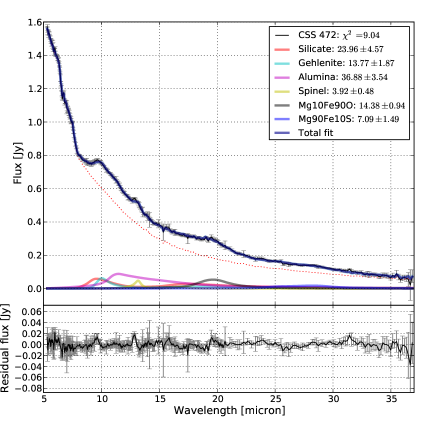
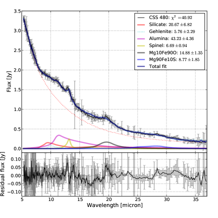
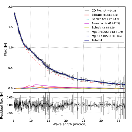
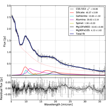
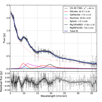
Figure 18: Continued

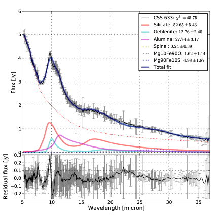
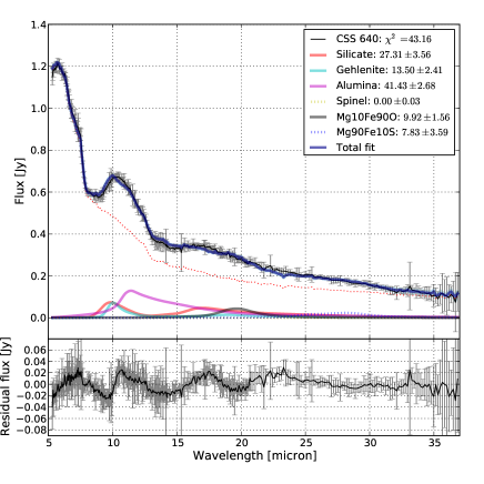
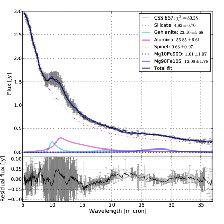
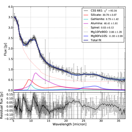
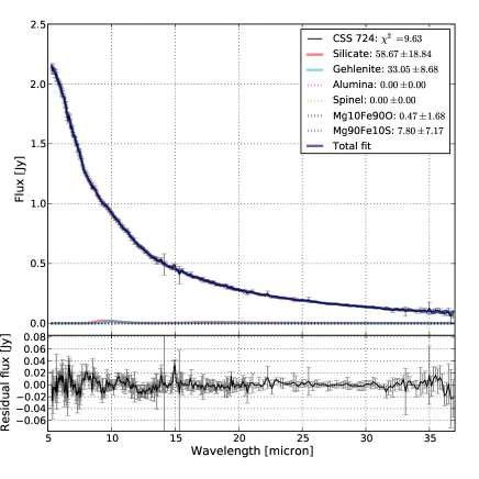
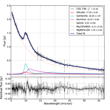
Figure 19: Continued

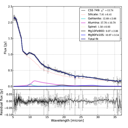
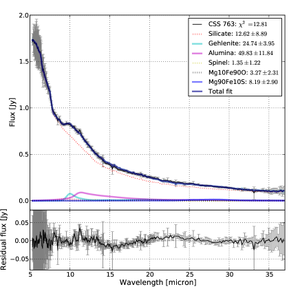
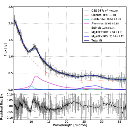
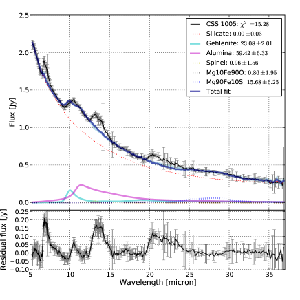
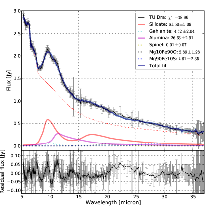
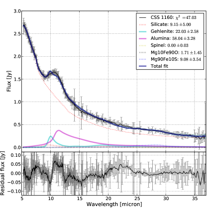
Figure 20: Continued

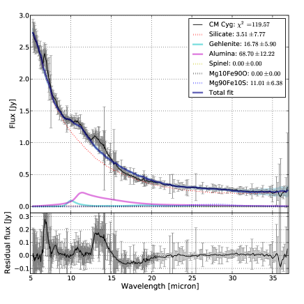
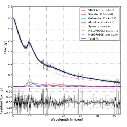
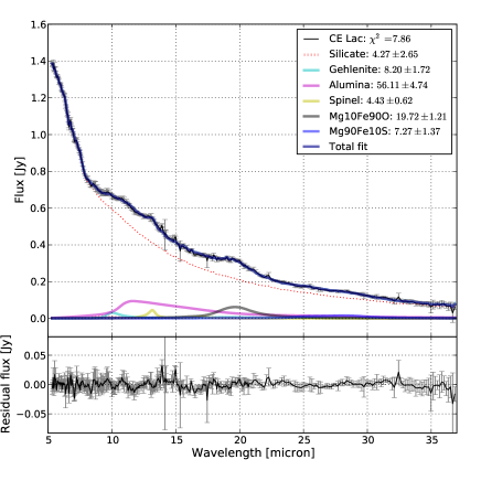
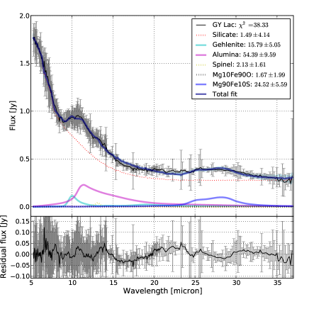
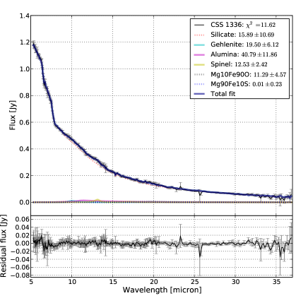
Figure 21: Continued