Joint analysis of X-ray and Sunyaev Zel’dovich observations of galaxy clusters using an analytic model of the intra-cluster medium

Abstract

We perform a joint analysis of X-ray and Sunyaev Zel’dovich (SZ) effect data using an analytic model that describes the gas properties of galaxy clusters. The joint analysis allows the measurement of the cluster gas mass fraction profile and Hubble constant independent of cosmological parameters. Weak cosmological priors are used to calculate the overdensity radius within which the gas mass fractions are reported. Such an analysis can provide direct constraints on the evolution of the cluster gas mass fraction with redshift. We validate the model and the joint analysis on high signal-to-noise data from the Chandra X-ray Observatory and the Sunyaev-Zel’dovich Array for two clusters, Abell 2631 and Abell 2204.

1. Introduction

Galaxy clusters trace the growth of structure in the universe. Their abundance and evolution is critically sensitive to underlying cosmological parameters such as $\Omega_{M}$, $\sigma_{8}$, and the dark energy equation of state parameter $w$. Recent work has focused on using galaxy clusters to constrain cosmology, including dark energy constraints from X-ray and joint X-ray/SZ measurements of the gas mass fraction (Allen et al., 2008; Ettori et al., 2009; LaRoque et al., 2006), cosmological parameter constraints from the growth of structure via X-ray (Mantz et al., 2008, 2010; Vikhlinin et al., 2009) and SZ cluster surveys (Vanderlinde et al., 2010; Marriage et al., 2011; Sehgal et al., 2010; Muchovej et al., 2011; Williamson et al., 2011; Benson et al., 2011).

In this paper, we present a method for the joint analysis of X-ray and SZ cluster observations using a self-consistent analytic model for the physical properties of the intra-cluster medium (Bulbul et al., 2010). The model provides analytic expressions for the radial density, temperature, and pressure profiles, and is therefore simultaneously applicable to both X-ray and SZ observables. The joint analysis allows measurement of the cluster gas mass fraction without the need to impose external priors on cosmological parameters such as the Hubble expansion rate $H(z)$. Such an analysis applied to a sample of clusters can directly probe the evolution of cluster gas mass fractions with redshift. We demonstrate the method using high signal-to-noise data from Chandra and Sunyaev-Zel’dovich Array (SZA) observations of two clusters, Abell 2631 and Abell 2204.

The method developed in this paper combines all available Chandra X-ray data (both imaging and spectroscopic) with SZ observations, using these to determine the angular diameter distance and cluster mass with minimal cosmological assumptions. We chose the Bulbul et al. (2010) model for this analysis since it describes the three thermodynamical cluster properties – density, temperature, and pressure – with a consistent set of parameters that are both readily interpreted. The temperature profile linking density and pressure is both easily calculated and observationally motivated. This work differs from Mroczkowski et al. (2009) who used SZ and X-ray imaging data only with a simplified, core-cut form of the Vikhlinin et al. (2006) model to describe the X-ray density and the Nagai et al. (2007) parameterization of the SZ pressure, and for which the inferred temperature profile did not reduce to a compact, accessible expression.

This paper is structured as follows: Section 2 describes the data reduction and analysis, Section 3 the modeling of X-ray and SZ data, and Section 4 the joint analysis of the X-ray and SZ data. We present and discuss our conclusions in Section 5.

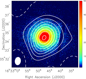
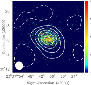
Figure 1.— SZ contours overlaid on X-ray false color images of Abell 2631 (left) and Abell 2204 (right ). The Chandra X-ray surface brightness data are from the energy range 0.7–7.0 keV. The color bars reflect the number of counts detected by Chandra in the 0.7-7 keV band, with a pixel size of 1.97 arcsec. The SZ data are from the SZA, and the contour levels are (+2,-2,-4,-6,-8,…) times the rms noise (see Table 1). The FWHM of the synthesized beams for these SZ observations are shown in the lower left corner of each image.

2. Data Reduction

We selected a non-cool core cluster (Abell 2631) and a cool-core cluster (Abell 2204) with high quality X-ray and SZ observations to demonstrate the method of analysis.

2.1. Chandra Imaging and Spectroscopy

The Chandra X-ray data are in the form of event files, which we use to generate both images and spectra. Additional blank-sky composite event files are used for background subtraction. The event files are reduced using CIAO 4.3.1 and CALDB 4.3, following the reduction procedure described in Bulbul et al. (2010). Details of each cluster observation can be found in Table 1.

The X-ray images in the 0.7-7 keV band are used to measure the X-ray surface brightness profile of the cluster. To subtract the background from the surface brightness, we rescale the blank-sky image to match the cluster surface brightness in a peripheral region that is free of cluster signal. The peripheral regions we chose are at a distance $\geq$ 500 arcsec from the cluster center for Abell 2631 (corresponding to 2.7 Mpc in the standard flat $\Lambda$CDM cosmology) and $\geq$ 550 arcsec (1.7 Mpc) for Abell 2204.

Spectra are extracted in annular regions centered at the peak of the X-ray emission. These regions cover an area out to the radius where the surface brightness profile reaches the background, which is near $r_{500}$ (the radius within which the average density is $500$ times the critical density at the cluster redshift) for these observations. From the blank-sky data, background spectra are also extracted and processed. We then rescale the blank-sky spectra to match the count rate of the cluster spectra in the 9.5-12 keV band. In this band, Chandra has no effective area for the detection of photons, and the detected counts originate from a particle background that is time variable. Hickox & Markevitch (2006) showed that while the flux within the 2–7 keV and 9.5–12 keV energy bands can vary with time, the ratio of the two bands remains constant. Subtracting the blank-sky data rescaled by the higher-energy band therefore accurately removes the background from the lower-energy band.

After rescaling the blank-sky spectra and removing the background from our cluster data, residuals may still be present in the soft 0.7–2 keV energy band. These soft X-ray residuals may be due to Galactic and extragalactic emission, and may vary as function of position (e.g., Snowden et al., 1997) and time (e.g., Takei et al., 2008). For each cluster observation, we use a peripheral region that is free of cluster emission—the same region used to rescale the background images—to determine whether soft residuals are present after the blank-sky background has been subtracted. We detect the presence of soft residuals in both clusters. The residual spectra are fit using a phenomenological model that includes a power law and a plasma emission model, and this model is rescaled by area and included in the spectral fit for each annulus (e.g., Snowden et al., 1998; Nevalainen et al., 2005; Maughan et al., 2008).

2.2. Interferometric Observations with the SZA

The two clusters were observed with the Sunyaev-Zel’dovich Array (SZA), an eight-element interferometer designed for the detection and imaging of the SZ effect. Each antenna in the array is 3.5 m in diameter and has a primary beam FWHM of 10.7^′ at the center frequency of the observing band (31 GHz). For these observations, six antennas were closely packed together to provide sensitivity to arcminute-scale SZ signals, and the remaining two antennas were placed further out to constrain the flux contributions from unresolved radio sources, as described in Muchovej et al. (2007). The unflagged on-source time for Abell 2631 was 16.1 hours and 19.6 hours for Abell 2204.The details of the observations are given in Table 1, and the radio sources detected in each field are listed in Table 2. In the analysis of the cluster SZ effect described below, the parameters of the SZ decrement and the radio sources are fit simultaneously.

The SZA data are reduced using a set of routines written in MATLAB that constitute a complete pipeline for flagging, calibrating, and reducing visibility data. The reduction pipeline, described in Muchovej et al. (2007), converts the data to physical units and corrects for instrumental phase and amplitude variations. Data are flagged for corruption due to bad weather, sources of radio interference, and other instrumental effects that could impact their quality. The pipeline outputs calibrated unflagged visibilties, i.e., components of the Fourier transform of the sky brightness multiplied by the primary beam response, along with their corresponding statistical weights and positions in the Fourier ($u-v$) plane.

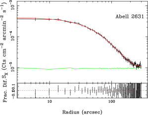
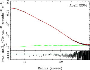
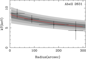
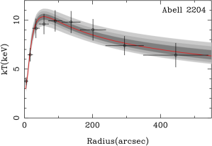
Figure 2.— X-ray surface brightness and temperature profiles for Abell 2631 (left column) and Abell 2204 (right column). Top panels: Surface brightness profiles where the black points are derived from the X-ray images, the red line shows the best fit model, and the green line is the background level determined from the blank sky observations. The residuals show the fractional difference between the model and the data. A $1\%$ systematic uncertainty has been added in quadrature to the datapoints. We plotted the surface brightness profiles beyond the fitted region to show the agreement between the cluster emission and background. Bottom panels: Temperature profiles where the red line shows the best fit model and the dark, medium, and light grey regions show the 68%, 95.4%, and 99.7% confidence levels obtained from the model fits. A $10\%$ systematic uncertainty has been added in quadrature to the temperature bins.

3. Modeling the X-ray and SZ data

The X-ray observable is spatially resolved spectroscopy, and temperature and metallicity of the intracluster plasma are measured using the X-ray spectroscopic data. The X-ray surface brightness is defined as

$$\mbox{$S_{\mbox{\tiny X}}$}=\frac{1}{4\pi(1+z)^{3}}\int n_{e}^{2}\mbox{$\Lambda_{ee}$}(T_{e},A)d\ell$$ (1)

where $\ell$ is the line of sight through the cluster, $n_{e}$ is the electron density, $T_{e}$ is the electron temperature, $A$ is the metallicity, and $\mbox{$\Lambda_{ee}$}(T_{e},A)$ is the X-ray cooling function (in units of counts cm³ s^-1) as a function of electron temperature and metallicity. The density, temperature, and metallicity can vary along the line of sight.

The observable from the SZ data is the amplitude of the spectral distortion of the Cosmic Microwave Background (CMB) in the direction of the cluster. This distortion is due to inverse Compton scattering of CMB photons off electrons in the intracluster medium (ICM), and results in a decrement in the CMB brightness temperature at frequencies $\lesssim~{}218$ GHz. The magnitude of the decrement is proportional to the electron pressure integrated along the line of sight (Sunyaev & Zel’dovich, 1972):

$$\Delta\mbox{$T_{\mbox{\tiny SZ}}$}=\mbox{$T_{\mbox{\tiny CMB}}$}\int\mbox{$\sigma_{\mbox{\tiny T}}$}f(x,T_{e})n_{e}\frac{kT_{e}}{m_{e}c^{2}}d\ell$$ (2)

where $T_{\mbox{\tiny CMB}}$ is the temperature of the CMB, $f(x,T_{e})$ contains the frequency dependence of the SZ temperature signature using the relativistic corrections provided by Itoh et al. (1998) and Nozawa et al. (2006), $\sigma_{\mbox{\tiny T}}$ is the Thomson cross section, $m_{e}$ is the electron mass, and $c$ is the speed of light.

Assuming spherical symmetry, the line of sight integration element $d\ell$ relates to the angular element (in radians) as $d\ell=\mbox{$D_{\mbox{\tiny A}}$}d\theta$, where $D_{\mbox{\tiny A}}$ is the angular diameter distance. From Equations 1 and 2, we find

$$S_{x}\propto\int D_{A}n_{e}^{2}\mbox{$\Lambda_{ee}$}(T_{e},A)d\theta$$ (3)

$$\Delta\mbox{$T_{\mbox{\tiny SZ}}$}\propto\int D_{A}n_{e}T_{e}d\theta.$$ (4)

The combination of X-ray imaging spectroscopy and SZ observations can be used to simultaneously measure the distribution of the electron density, the electron temperature, and the angular diameter distance (e.g., Hughes & Birkinshaw, 1998; Grego et al., 2000; Reese et al., 2002; Grainge et al., 2002; Saunders et al., 2003; Bonamente et al., 2006). For further discussion on the SZ effect and its use for cosmology, see reviews by Birkinshaw (1999) and Carlstrom et al. (2002).

We describe the density and temperature profiles of the hot plasma in galaxy clusters using the model proposed by Bulbul et al. (2010):

$$n_{e}(r)=n_{e0}\phi(r,r_{s},\beta)^{n}\tau_{cool}^{-1}$$ (5)

$$T(r)=T_{0}\phi(r,r_{s},\beta)\tau_{cool}$$ (6)

where

$$\phi(r,r_{s},\beta)=\frac{1}{(\beta-2)}\frac{(1+r/r_{s})^{\beta-2}-1}{r/r_{s}(1+r/r_{s})^{\beta-2}},$$ (7)

$$\tau_{cool}=\frac{\alpha+(r/r_{\rm cool})^{\gamma}}{1+(r/r_{\rm cool})^{\gamma}},$$ (8)

$n_{e0}$ is the normalization of the pressure profile, $n$ is the polytropic index, $r_{s}$ is the scale radius, $T_{0}$ is the normalization factor for the scaling of the temperature profile, $\gamma$ is the slope of the cooling function, and $\alpha$ is the cooling parameter which ranges from 0 to 1. One attractive feature of these models is that they provide a simple analytic form for the electron pressure:

$$P_{e}(r)=P_{e0}\phi(r,r_{s},\beta)^{n+1},$$ (9)

where $P_{e0}=n_{e0}kT_{0}$ is the pressure normalization. The free parameters of the model, which are used to jointly fit the X-ray and SZ data, are $n_{e0},T_{0},r_{s},r_{\rm cool},\alpha,\beta,\gamma,n$ and the distance $D_{A}$.

Parameter estimation is done using a Monte Carlo Markov chain (MCMC) method described in Bonamente et al. (2004). Correlation among model parameters is a feature of most analytic models, including the one used in this paper. Parameter correlations can result in low acceptance rates and thus slow convergence of the Markov chains (e.g., Gilks et al., 1996). In our implementation, steps of the MCMC are proposed along the set of directions which diagonalize the covariance of the posterior distribuition, determined via singular-value decomposition of an initial test chain, resulting in efficient exploration of the parameter space (see Appendix).

Figure 3.— SZ visibility profiles for Abell 2631 (top) and Abell 2204 (bottom) plotted as a function of $u-v$ radius ($\sqrt{u^{2}+v^{2}}$). The plots show the real components of the measured $Y(u,v)$ along with the best fit model.

3.1. X-ray Data Analysis

The annular bins in the temperature profile (Figure 2) were chosen by starting with an initial 10^′′ bin and then increasing each bin by 50% of the width of the previous bin to give roughly the same counts per bin. Following the analysis of the systematic uncertainties for the X-ray data described in Bulbul et al. (2010), we adopt a 1% systematic uncertainty on the count rate of each bin of the surface brightness profile and a 10% systematic uncertainty on the temperature of each spectral region as discussed in Section 4.5.1. Figure 2 shows the temperature and surface brightness profiles, along with the best-fit models, for the fit to the X-ray data only of Abell 2631 and Abell 2204. Since our model has the same parameters for both density and temperature, the surface brightness profile carries a larger weight in the fit. The model fits are acceptable for both clusters to within the plotted errors, which include the systematic uncertainties associated with the surface brightness and temperature discussed in Section 4.5. For Abell 2631, there is insufficient signal to constrain $n$ and $\beta$ simultaneously. In this case, we fix $\beta=2$, which is equivalent to assuming that the total mass follows a Navarro et al. (1997) profile at large radii (see Section 4.3).

3.2. SZ Data Analysis

After removal of compact radio sources in the cluster field, the visibilities $V_{\nu}(u,v)$ measured by the SZA can be related to the Fourier domain equivalent of the integrated Compton-$y$ parameter $Y(u,v)$ (see, e.g., Mroczkowski et al., 2009). This is defined as

$$Y(u,v)\equiv\frac{V_{\nu}(u,v)}{g(x)\,I_{0}},$$ (10)

where $g(x)$ corrects for the frequency dependence of the SZ flux, and $I_{0}=2(k_{B}\mbox{$T_{\mbox{\tiny CMB}}$})^{3}/(hc)^{2}$ is the primary CMB intensity normalization. Figure 3 shows $Y(u,v)$ along with the best-fit model, for the fit to the SZ data only of the two clusters.

4. Joint Analysis of X-ray and SZ Data

We first perform a consistency check of the determination of the pressure profiles from the X-ray and SZ data. We then focus on determinations of the angular diameter distance and the radial profile of the gas mass fraction using the consistent parameterization of density, temperature and pressure provided by the ICM model for the joint analysis of the X-ray and SZ observables.

4.1. Consistency of X-ray and SZ measurements of the electron pressure profiles

X-ray and SZ observations provide independent measurements of the radial distribution of the electron pressure. The X-ray observables are the electron temperature and surface brightness, the latter depends on the square of the electron density according to Equation 1; the SZ observable, on the other hand, is directly proportional to the electron pressure integrated along the line of sight (Equation 2).

The two observables can be affected by different sources of systematic uncertainties. For example, the presence of non-thermal X-ray emission (e.g., Million & Allen, 2009; Bonamente et al., 2005; Sarazin & Lieu, 1998) could result in the increase of the X-ray emission above the level of the thermal gas, and radio emission from cluster halos (e.g., Brunetti et al., 2007) may partially fill the SZ decrement. Another source of systematic uncertainty is the assumption of spherical symmetry in the analysis (e.g., Sulkanen, 1999), which would result in a different measurement of the pressure from X-ray and SZ observations. A discussion of sources of systematic uncertainty in the analysis of X-ray and SZ observations is presented in Section 4.5. A comparison of the pressure profiles from SZ and X-ray observations is therefore useful to determine the presence of sources of emission that can cause differences between the two measurements.

We perform a joint fit to the X-ray and SZ data using Equation 9, with the normalization of the SZ pressure model independent of the X-ray density and temperature normalizations. The common parameters in the models ($r_{s}$, $\beta$, and $n$) are linked between the two datasets, thus requiring the X-ray and SZ pressure profiles to have the same shape. In this analysis, we adopt the angular diameter distance appropriate for the cluster redshift in a $\Lambda$CDM model with $h=0.73$, $\Omega_{M}=0.27$ and $\Omega_{\Lambda}=0.73$.

The pressure inferred from the X-ray and SZ measurements are within 20% of one another for both clusters, consistent with the statistical and systematic effects (Tables 3 and 6); results for a larger sample of clusters can be found in Bonamente et al. (2011). Note that the measurement of the ratio of X-ray pressure to the SZ pressure depends on the choice of the Hubble parameter, since the pressure normalizations are degenerate with the value of $D_{A}$ assumed in the analysis.

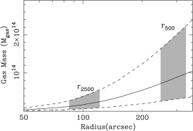
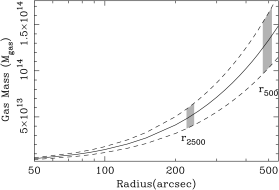
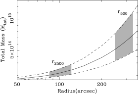
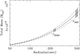
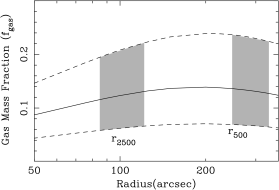
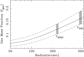
Figure 4.— Top Panels; left Abell 2631, right Abell 2204: Gas mass profiles determined from the joint analysis of Chandra/SZA observations for Abell 2631 and Abell 2204. Middle Panels: Total mass profiles. Bottom Panels: Gas mass fraction profiles. The dashed lines are the 68% confidence level at each radius. Grey areas show the measurements at radii $r_{2500}$ and $r_{500}$, obtained by marginalization over the cosmological parameters. Chandra calibration systematics are included in the measurements.

4.2. Direct measurement of the angular diameter distance

We also perform a joint X-ray and SZ analysis which enables us to place direct constraints on the angular diameter distance without using priors on the cosmological parameters (e.g., Hughes & Birkinshaw, 1998; Birkinshaw, 1999; Reese et al., 2002; Bonamente et al., 2006). For this analysis, we link the shape parameters and the pressure normalizations between the X-ray and SZ data, and allow $D_{A}$ to vary. For Abell 2631 and Abell 2204 we measure $D_{A}=798.9\pm^{308.1}_{267.4}\rm{Mpc}$ and $D_{A}=575.3\pm^{46.6}_{55.6}\rm{Mpc}$, both values are consistent with those calculated using a standard a $\Lambda$CDM cosmology at the 1–$\sigma$ level. The measurement of the $D_{A}$ for Abell 2204 is also in agreement with that of Bonamente et al. (2006). The measurement of the angular diameter distance for a given cluster is affected by a number of systematic effects (Bonamente et al., 2006), and the agreement of $D_{A}$ with the $\Lambda$CDM value is expected for a large sample but not necessarily for individual clusters, as it is for the two clusters in this paper.

4.3. Radial profiles of the gas mass fraction independent of cosmological parameters

By using direct measurement of $D_{A}$ as described in Section 4.2, we can also obtain radial profiles of the gas mass, total mass, and the gas mass fraction without the need to use priors on the cosmological parameters. The gas mass $M_{\mbox{\scriptsize gas}}$ is computed by integrating the gas density profile within the volume,

$$\mbox{$M_{\mbox{\scriptsize gas}}$}=4\pi\mu_{e}m_{p}\int n_{e}(r)r^{2}dr=4\pi\mu_{e}m_{p}\mbox{$D_{\mbox{\tiny A}}$}\!^{3}\int n_{e}(\theta)\theta^{2}d\theta,$$ (11)

where $\mu$ is the mean molecular weight (calculated assuming metal abundances of $0.3$ solar, Anders & Grevesse 1989), $m_{p}$ is the proton mass, and $dr=\mbox{$D_{\mbox{\tiny A}}$}d\theta$. The total mass $M_{\mbox{\scriptsize tot}}$ is computed assuming hydrostatic equilibrium between the gravitational mass and the thermal pressure of the gas:

$$\mbox{$M_{\mbox{\scriptsize tot}}$}(r)=\frac{4\pi\rho_{i}r_{s}^{3}}{(\beta-2)}\left(\frac{1}{\beta-1}+\frac{1/(1-\beta)-r/r_{s}}{(1+r/r_{s})^{\beta-1}}\right)\tau_{cool}(r),$$ (12)

where $\rho_{i}=(T_{0}k(n+1)(\beta-1))/(4\pi G\mu m_{p}r_{s}^{2})$.

Figure 4 shows the radial profiles of the gas mass, total mass, and gas mass fraction for Abell 2631 and Abell 2204. The uncertainties reflect the fact that $D_{A}$ is also measured directly from the data, and that no assumption about the value of the cosmological parameters $H_{0}$, $\Omega_{M}$ or $\Omega_{\Lambda}$ was made.

4.4. Measurement of the gas mass fraction at an overdensity radius

In cosmological applications (e.g., via the distribution of $f_{\mbox{\scriptsize gas}}$ with redshift, Allen et al., 2008) $f_{\mbox{\scriptsize gas}}$ is typically measured within an overdensity radius. The radius $r_{\Delta}$ is defined as the radius within which the average matter density of the cluster is $\Delta$ times the critical density of the universe at the cluster’s redshift:

$$r_{\Delta}^{3}\equiv\frac{\mbox{$M_{\mbox{\scriptsize tot}}$}(r_{\Delta})}{\frac{4\pi}{3}\Delta\rho_{c}(z)},$$ (13)

where $\rho_{c}(z)=(3H_{0}^{2}E^{2}(z))/(8\pi G)$ is the critical density of the universe, $H_{\mbox{\tiny 0}}$ is the Hubble constant, and $E^{2}(z)$= $\mbox{$\Omega_{\mbox{\scriptsize M}}$}(1+z)^{3}+\mbox{$\Omega_{\Lambda}$}+\mbox{$\Omega_{\mbox{\scriptsize k}}$}(1+z)^{2}$ in the $\Lambda$CDM model.

The joint X-ray and SZ analysis provides cosmology-independent constraints on $D_{A}$ and on the radial profile of $\mbox{$f_{\mbox{\scriptsize gas}}$}(r)$ (Sections 4.2 and 4.3). The radius $r_{\Delta}$ and therefore all quantities calculated out to this radius retain a cosmological dependence through the factor $\rho_{c}(z)$ appearing in Equation 13. In the following we describe a method to marginalize the measurement of $f_{\mbox{\scriptsize gas}}$($r_{\Delta}$) over the cosmological parameters, which results in a weak cosmology dependence of our joint measurements of $f_{\mbox{\scriptsize gas}}$($r_{\Delta}$).

In what follows, we adopt the standard flat Friedman-Robertson-Walker (FRW) cosmological model, parameterized by $H_{0}$ and $\Omega_{\mbox{\scriptsize M}}$, with $\mbox{$\Omega_{\Lambda}$}=1-\mbox{$\Omega_{\mbox{\scriptsize M}}$}$, which is known to provide a good fit to other cosmic distance data (Allen et al., 2008; Freedman et al., 2009; Percival et al., 2010). Within this model, a given $D_{A}$ value corresponds to a curve in the ($H_{0}$, $\Omega_{\mbox{\scriptsize M}}$) plane described by

$$H_{0}=\frac{c}{D_{A}(1+z)}\int_{0}^{z}\frac{d\zeta}{[\Omega_{M}((1+\zeta)^{3}-1)-1]^{1/2}},$$ (14)

where spatial flatness is assumed. For each step in the Markov chain of each cluster, we use the corresponding value of $D_{A}$ to generate a consistent pair of cosmological parameters by drawing a random value of $\Omega_{\mbox{\scriptsize M}}$ from a uniform distribution on [0,1], and calculating the associated value of $H_{0}$ from Equation 14. We then use these parameters when calculating $r_{\Delta}$ and the other fit parameters of the chain. This approach has the advantage of using minimal prior information on the cosmological parameters, with $\Omega_{\mbox{\scriptsize M}}$ free to range between 0 and 1, and $D_{A}$ measured directly from the data. This method properly accounts for the covariance between $r_{\Delta}$, $\mbox{$f_{\mbox{\scriptsize gas}}$}(r_{\Delta})$, $D_{A}$ and the other parameters of the fit. For the flat FRW model and the low redshifts in question, this procedure corresponds, to very good approximation, to the use of uniform priors on $H_{0}$ and $\Omega_{\mbox{\scriptsize M}}$. We note, however, that this correspondence does not necessarily hold for higher redshifts ($z\sim$1) or for other cosmological models. The measurements of masses and $f_{\mbox{\scriptsize gas}}$ at $r_{2500}$ and $r_{500}$ are indicated as grey areas in Figure 4 and are listed in Table 4.

For comparison, we also provide the measurements of masses and $f_{\mbox{\scriptsize gas}}$ using the X-ray data with a fixed $D_{A}$ calculated from the standard flat $\Lambda$CDM cosmology, and priors on $\Omega_{M}$ from the WMAP measurements of Komatsu et al. (2011). The results are reported in Table 5.

4.5. Sources of Systematic Uncertainty

The sources of systematic uncertainty on the gas mass fraction and the integrated X-ray and SZ pressure are listed in Table 6. The individual errors are added in quadrature to determine the total systematic uncertainty on $f_{gas}$ and the integrated pressure. Systematics from Chandra instrument calibration and the X-ray background are included in the fitting of the data, and the value of masses and $f_{gas}$ in Tables 4 and 5 account for these systematics. Since this joint analysis method can be applied to larger samples of clusters, we also indicate whether the impact of each source of systematic uncertainty is reduced with sample size.

4.5.1 Instrument Calibration

Chandra’s ACIS effective area has a spatially dependent non-uniformity at the level of $\pm 1\%$ and therefore we add a $\pm 1\%$ uncertainty to the surface brightness data. We also adopt a $\pm 10\%$ uncertainty on the temperature measurements to account for uncertainty in the low-energy calibration of the effective area (see, e.g., Bulbul et al., 2010). These uncertainty estimates for the Chandra calibration are folded into the mass measurements reported in Tables 3, 4 and 5.

Frequent observations of Mars are used to calibrate the SZA absolute flux scale; we employ the Rudy (1987) flux model which has an estimated absolute calibration uncertainty of $\pm 5\%$. The stability of the instrumental gain is $\pm 3\%$, as determined from repeated calibrator measurements in SZA survey fields (Muchovej et al., 2011). The absolute calibration and instrumental gain yield a global $\pm 6\%$ uncertainty on the SZA calibration. We rescaled the SZA data by the $\pm 6\%$ uncertainty on the SZA calibration and compared the measurements to the original analysis. We found a $\pm 6\%$ systematic uncertainty on the pressure and $\pm 10\%$ systematic uncertainty on the gas mass fraction at $r_{2500}$ and $r_{500}$. The uncertainty associated with instrument calibration does not average down with sample size.

4.5.2 Kinetic SZ Effect

Reese et al. (2002) reports that for a cluster with a temperature of 8.0 keV and with a typical velocity along the line of sight of 300 km/s (Watkins, 1997; Colberg et al., 2000) the kinetic SZ effect would be $\pm 4\%$ of the thermal SZ for 30 GHz observations. Accordingly we use a $\pm 4\%$ uncertainty due to the kinetic SZ effect on the gas mass fraction and the SZ pressure profiles for measurements at $r_{2500}$ and $r_{500}$. This source of uncertainty averages down by a factor of the square root of the size of the sample.

4.5.3 Radio Source Contamination

Undetected radio sources not accounted in the modeling could lead to a biased measurement of the SZ decrement. We use the Faint Images of the Radio Sky at Twenty-centimeters (FIRST) database as a reference for locating compact radio sources within 10^′ of the cluster center. Most radio sources that will affect the 30 GHz data (rms noise $\sim$ 0.25 mJy) will have counterparts in the FIRST survey (rms noise of 0.15 mJy at 1.4 GHz); inverted spectrum sources may not have counterparts at 1.4 GHz and will affect our measurement of the SZ decrement, but they comprise a small fraction of the source population (Muchovej et al., 2010, Fig. 3).

We determine the effect of undetected point sources by placing a radio source model at each FIRST source, fixing the position and marginalizing over the flux. In the pressure model (Equation 7), we fixed the parameters $r_{s}$, $n$, $\beta$, and $D_{A}$ and let $P_{eo}$ be free. We compare the pressure profiles with the original analysis (see Table 2) and find a $\leq 1\%$ difference in the pressure of each cluster. Therefore we conservatively apply a $1\%$ uncertainty on the pressure and $2\%$ uncertainty on the gas mass fraction at $r_{2500}$ and $r_{500}$.

4.5.4 Asphericity

Although we assume a spherical model in our analysis, most clusters do not appear to be circular in shape in X-ray or radio observations. LaRoque et al. (2006) reports a $10-20\%$ uncertainty in the measurement of the gas mass fraction due to asphericity; therefore we use $\pm 20\%$ as a conservative estimate for measurements at $r_{2500}$ and $r_{500}$. This uncertainty also averages down by a factor of the square root of the sample size, as shown in Sulkanen (1999), provided the selection of the sample is unbiased with respect to cluster shape.

4.5.5 Hydrostatic Equilibrium Assumption

The assumption of hydrostatic equilibrium at large radii results in an underestimate of the total mass. This is due to the presence of non-thermal pressure which can bias hydrostatic equilibrium measurements of the total mass (Evrard et al. 1990). According to Lau et al. (2009) the total mass of a relaxed cluster such as Abell 2204 will be biased by $-6\%$ at $r_{2500}$ and $-8\%$ at $r_{500}$, and for unrelaxed systems such as Abell 2631 by $-9\%$ at $r_{2500}$ and $-11\%$ at $r_{500}$. Therefore we adopt a systematic uncertainty of $-9\%$ and $-11\%$ in our error analysis for measurements at $r_{2500}$ and $r_{500}$.

4.5.6 X-ray Background

The X-ray background is determined from the ACIS blank sky composite event file. We normalize the blank sky background level for each observation using an emission-free region on the ACIS detector. We adjusted the background normalization factor by a factor of $\pm 2\sigma$ and propagated this through the analysis, and found that this produces a $\pm 2\%$ uncertainty on the background count rate. This uncertainty affects the surface brightness and temperature measurements resulting in a $\pm 2\%$ and $\pm 9\%$ uncertainty on the gas mass fraction measurements at $r_{2500}$ and $r_{500}$, and a $\pm 2\%$ uncertainty on the X-ray pressure profiles at both radii. This uncertainty averages down by a factor of the square root of the sample size.

4.5.7 Systematics associated with the use of the Bulbul et al. (2010) models

The Bulbul et al. (2010) model assumes a polytropic relationship between the ICM density and temperature at large radii. To estimate uncertainties associated with the polytropic assumption, we compare our X-ray masses for the two clusters in our sample with those calculated using the Vikhlinin et al. (2006) model, which provides an independent parameterization of the thermodynamic quantities. From this comparison, we find that the gas mass fraction measurements varies by $\leq 10\%$ at all radii between the Bulbul et al. (2010) and Vikhlinin et al. (2006) models. We estimate the uncertainty on the corresponding pressure profiles by comparing the integrated pressures between the two models, and the comparison results in an uncertainty of $\pm 3\%$ at $r_{2500}$ and $\pm 5\%$ at $r_{500}$. We consider these uncertainties as a rough estimate of the systematics associated with the Bulbul et al. (2010) model.

4.5.8 Helium Sedimentation

The effect of helium sedimentation may be an additional source of systematic uncertainty. In our measurements we assume that the hydrogen to helium ratio is uniform throughout the cluster. However, theoretical studies (Fabian & Pringle, 1977; Rephaeli, 1978) suggest helium sedimentation effects may affect cluster mass measurements. Peng & Nagai (2009) finds that the bias in gas mass fraction from the presence of helium sedimentation is less than 10% at $\sim r_{2500}$ and negligible at $r_{500}$. Accordingly, we estimate a systematic uncertainty of 10% at $r_{2500}$ and $\leq$5% at $r_{500}$ for the measurement of the gas mass fraction. Bulbul et al. (2011) applied the Peng & Nagai (2009) helium sedimentation simulation model to a sample of clusters and demonstrated the effects on the gas mass and total mass. The integrated pressure is proportional to the gas mass, and we use the values from Bulbul et al. (2011) to determine upper limits to the systematic uncertainty in the measurement of pressure of $-4\%$ at $r_{2500}$ and $-2\%$ at $r_{500}$.

5. Conclusions

We demonstrate the use of the Bulbul et al. (2010) cluster model for simultaneous fitting of X-ray data and Sunyaev-Zel’dovich effect data. The model employs a compact parameterization that relates the three primary thermodynamic quantities by the ideal gas law at all radii. We consider X-ray data from Chandra and 30-GHz SZ data from the SZA for both clusters, Abell 2631 and Abell 2204 and find that the model adequately captures the radial variation in both the X-ray surface brightness and SZ Compton-$y$ profiles. For all clusters, separate determinations of the electron pressure from the X-ray and SZ data yield profiles that are statistically consistent.

Joint analysis of the X-ray and SZ data provides a direct measure of $D_{A}$, the angular diameter distance to the cluster, that is independent of cosmology. For both clusters, this analysis yields a measure of $D_{A}$ that is consistent with the standard $\Lambda$CDM values at the 1-$\sigma$ level. Using the measured angular diameter distance as a constraint between $H_{0}$ and $\Omega_{\mbox{\scriptsize M}}$, we marginalize over the implicit cosmology dependence of the overdensity radius to obtain estimates of $f_{\mbox{\scriptsize gas}}$ at $r_{2500}$ and $r_{500}$ that are only weakly dependent on $\Omega_{\mbox{\scriptsize M}}$.

We discuss possible sources of systematic errors in the $f_{\mbox{\scriptsize gas}}$ determination, and find that most will be mitigated if $f_{\mbox{\scriptsize gas}}$ is averaged over a large sample of clusters. A sample spanning a large redshift range can be used to constrain the evolution of $f_{\mbox{\scriptsize gas}}$ with redshift, and for constraining cosmological models with clusters (e.g., Sasaki, 1996; Pen, 1997; Reese et al., 2002; Allen et al., 2004; LaRoque et al., 2006; Bonamente et al., 2006; Allen et al., 2008; Ettori et al., 2009).

Table 1Cluster Observations

Cluster	$z$	$n_{H}$	$RA$	$Dec$	Chandra Observations		SZA Observations
		$(10^{20}\rm cm^{-2})$	(J2000)	(J2000)	ObsID	Time	On-src Time	FWHM	P.A.	rms Noisea
						(ks)	(hrs)	(arcsec)	(deg)	(mJy)
A2631	0.27	3.55	23:37:40.1	+00:16:33	3248/11728	25.0	16.1	$152\times 117$	17.2	0.4
A2204	0.15	5.67	16:32:47.2	+05:34:32	7940	72.9	19.6	$157\times 115$	-7.7	0.4

Table 2Radio Sources in Cluster Fields

Cluster	Pointing Center		30 GHz Source
	$RA$	$Dec$	src	$\Delta\alpha^{a}$	$\Delta\delta^{a}$	Flux	FWHM	P.A.	rms Noiseb
	(J2000)	(J2000)		(arcsec)	(arcsec)	(mJy)	(arcsec)	(deg)	(mJy)
Abell 2631	23:37:38.8	+00:16:06.5	1	21.3	36.5	3.7	$26.5\times 16.6$	42.7	0.25
			2	205.0	-130.0	0.5
Abell 2204	16:32:46.88	+05:34:32.4	1	0.4	1.2	7.0	$21.1\times 18.4$	-82.1	0.22
			2	-417.8	-360.1	21.6
			3	195.0	-130.1	0.7

Table 3Pressure Normalization Values and Integrated $Y(r_{500})$ Values^a

Cluster	$P_{eo}(SZ)$	$P_{eo}(X)$	$P_{eo}(SZ)/P_{eo}(X)$
	($10^{-10}~{}\mathrm{ergs~{}cm^{-3}}$)
Abell 2631	$1.00\pm^{0.11}_{0.11}$	$1.21\pm^{0.15}_{0.14}$	$0.82\pm^{0.09}_{0.09}$
Abell 2204	$9.90\pm^{0.60}_{0.60}$	$9.71\pm^{0.47}_{0.47}$	$1.02\pm^{0.05}_{0.05}$
	$Y_{\rm sph,SZ}(r_{500})$	$Y_{\rm sph,X}(r_{500})$	$Y_{\rm sph,SZ}(r_{500})/Y_{\rm sph,X}(r_{500})$
	($10^{-11}$)
Abell 2631	$9.13\pm^{1.17}_{1.00}$	$11.13\pm^{1.52}_{1.34}$	$0.82\pm^{0.15}_{0.18}$
Abell 2204	$44.97\pm^{2.99}_{2.74}$	$43.93\pm^{3.08}_{2.59}$	$1.02\pm^{0.10}_{0.09}$

Table 4Results from Joint X-ray/SZ Analysis

	Model Parameters
Cluster	$n_{e0}$	$r_{s}$	$n$	$\beta$	$T_{\rm\tiny 0}^{a}$	$r_{\rm cool}$	$\alpha$	$\gamma^{b}$	$D_{\mbox{\tiny A}}$
	($10^{-2}$cm-3)	(arcsec)			(keV)	(arcsec)			(Mpc)
Abell 2631	$0.78\pm^{0.17}_{0.12}$	$261.1\pm^{74.6}_{50.2}$	$9.6\pm^{2.1}_{1.4}$	$2.0$	$7.6\pm^{1.7}_{1.6}$	-	-	-	$799\pm^{308}_{267}$
Abell 2204	$3.90\pm^{0.25}_{0.19}$	$22.7\pm^{1.8}_{1.9}$	$6.9\pm^{1.8}_{1.3}$	$1.37\pm^{0.10}_{0.08}$	$14.9\pm^{1.6}_{0.9}$	$20.0\pm^{0.7}_{0.7}$	$0.17\pm 0.01$	$2.0$	$575\pm^{47}_{56}$
	Cluster Massesc
	Masses Evaluated At $\Delta$= 2500				Masses Evaluated At $\Delta$=500
Cluster	$r_{\Delta}$	$M_{\mbox{\scriptsize gas}}$	$M_{\mbox{\scriptsize tot}}$	$f_{\mbox{\scriptsize gas}}$	$r_{\Delta}$	$M_{\mbox{\scriptsize gas}}$	$M_{\mbox{\scriptsize tot}}$	$f_{\mbox{\scriptsize gas}}$
	(”)	$(10^{13}M_{\odot})$	$(10^{14}M_{\odot})$		(”)	$(10^{13}M_{\odot})$	$(10^{14}M_{\odot})$
Abell 2631	$103.2\pm^{18.4}_{18.3}$	$1.71\pm^{2.40}_{1.16}$	$1.37\pm^{1.16}_{0.65}$	$0.124\pm^{0.081}_{0.060}$	$289.3\pm^{44.0}_{41.6}$	$8.35\pm^{10.77}_{5.33}$	$6.16\pm^{4.35}_{2.62}$	$0.131\pm^{0.103}_{0.065}$
Abell 2204	$231.3\pm^{9.0}_{8.3}$	$5.03\pm^{1.08}_{1.07}$	$4.09\pm^{0.39}_{0.34}$	$0.122\pm^{0.019}_{0.018}$	$492.6\pm^{23.3}_{20.7}$	$13.09\pm^{2.96}_{2.94}$	$7.95\pm^{1.20}_{0.92}$	$0.161\pm^{0.026}_{0.021}$

Table 5Results from X-ray Analysis

	Model Parameters
Cluster	$n_{e0}$	$r_{s}$	$n$	$\beta$	$T_{\rm\tiny 0}^{a}$	$r_{\rm cool}$	$\alpha$	$\gamma^{b}$	$D_{\mbox{\tiny A}}$b
	($10^{-2}$cm-3)	(arcsec)			(keV)	(arcsec)			(Mpc)
Abell 2631	$0.7r\pm^{0.03}_{0.03}$	$248.0\pm^{67.6}_{47.0}$	$9.27\pm^{1.91}_{1.34}$	$2.0$	$8.3\pm^{0.7}_{0.7}$	-	-	-	$840.0$
Abell 2204	$4.12\pm^{0.23}_{0.25}$	$22.5\pm^{1.7}_{1.5}$	$6.76\pm^{1.19}_{0.82}$	$1.38\pm^{0.06}_{0.06}$	$15.0\pm^{0.8}_{0.8}$	$20.0\pm^{0.7}_{0.6}$	$0.17\pm^{0.08}_{0.09}$	$2.0$	$526.0$
	Cluster Massesc
	Masses Evaluated At $\Delta$= 2500				Masses Evaluated At $\Delta$=500
Cluster	$r_{\Delta}$	$M_{\mbox{\scriptsize gas}}$	$M_{\mbox{\scriptsize tot}}$	$f_{\mbox{\scriptsize gas}}$	$r_{\Delta}$	$M_{\mbox{\scriptsize gas}}$	$M_{\mbox{\scriptsize tot}}$	$f_{\mbox{\scriptsize gas}}$
	(”)	$(10^{13}M_{\odot})$	$(10^{14}M_{\odot})$		(”)	$(10^{13}M_{\odot})$	$(10^{14}M_{\odot})$
Abell 2631	$113.9\pm^{6.6}_{7.0}$	$2.45\pm^{0.26}_{0.27}$	$1.98\pm^{0.37}_{0.35}$	$0.124\pm^{0.010}_{0.008}$	$309.9\pm^{20.7}_{18.3}$	$10.34\pm^{0.50}_{0.49}$	$8.00\pm^{1.72}_{1.33}$	$0.129\pm^{0.019}_{0.018}$
Abell 2204	$234.4\pm^{3.8}_{3.9}$	$4.12\pm^{0.09}_{0.09}$	$3.75\pm^{0.19}_{0.18}$	$0.110\pm^{0.003}_{0.003}$	$499.0\pm^{11.8}_{12.5}$	$10.64\pm^{0.27}_{0.29}$	$7.27\pm^{0.53}_{0.53}$	$0.146\pm^{0.007}_{0.007}$

Table 6Sources of Uncertainty

	$r_{2500}$			$r_{500}$
	Effect on $f_{\mbox{\scriptsize gas}}$	Effect on Pressure		Effect on $f_{\mbox{\scriptsize gas}}$	Effect on Pressure
Source	(%)	SZ (%)	X-ray (%)	(%)	SZ (%)	X-ray (%)
Kinetic SZ effect	$\pm 4$	$\pm 4$	…	$\pm 4$	$\pm 4$	…
Radio Point Sources	$\pm{2}$	$\pm{1}$	…	$\pm{2}$	$\pm{1}$	…
Asphericity	$\pm 20$	$\pm 10$	$\pm 10$	$\pm 20$	$\pm 10$	$\pm 10$
X-ray background	$\pm{5}$	…	$\pm{1}$	$\pm{9}$	…	$\pm{2}$
SZA calibration	$\pm{10}$	$\pm{6}$	…	$\pm{10}$	$\pm{6}$	…
Hydrostatic Equilibriuma	-9	…	…	-11	…	…
Model Assumptions	$\pm 10$	$\pm 3$	$\pm 3$	$\pm 10$	$\pm 5$	$\pm 5$
Helium Sedimentation	+10	…	-4	+5	…	-2
Total Systematic	$\pm{28}$	$\pm{13}$	$\pm{11}$	$\pm^{27}_{29}$	$\pm{14}$	$\pm{12}$
Chandra calibration uncertaintiesb
Surface Brightness	$\pm 10$
Temperature	$\pm 1$

Appendix: MCMC Reparameterization Using a Singular Value Decomposition Method

Correlation among model parameters is a common feature of analytic models such as the beta model (Cavaliere & Fusco-Femiano, 1976), the Vikhlinin et al. (2006) model, and the Bulbul et al. (2010) model used in this paper. The Monte Carlo Markov chain (MCMC) method for the analysis of X-ray and SZE data described in Bonamente et al. (2004) accounts for this correlation, and therefore correlation is not an issue when evaluating integrated quantities such as masses and $Y$ values, and their uncertainties. Strong parameter correlation, however, may cause the MCMC to be inefficient in its sampling of parameter space (see, e.g., Gilks et al., 1996, page 90), requiring long chains with low acceptance rate because of the poor mixing. A common solution is the use of a singular value decomposition (SVD, e.g., Press et al., 1992) to perform a linear transformation of the parameters to reduce the correlation among model parameters, and increase of the rate of acceptance in the Monte Carlo Markov chain. For the X-ray analysis of the Chandra data of Abell 2631 shown in Table 5, the four model parameters ($n_{e0}$, $r_{s}$, $n$ and $\beta$) are transformed into four SVD parameters ($svd_{0}$ through $svd_{3}$), and the usual Metropolis-Hastings MCMC is applied to the SVD parameters. The accepted parameters are then transformed back to the original Bulbul et al. (2010) model parameters, for which we calculate integrated quantities.

The effect of the reparameterization is shown in Figures 5 and 6. The strong correlation present between certain pairs of parameters, especially $r_{s}$ and $n$, is absent from the SVD parameters.

Figure 5.— Scatter plot for parameters of the Bulbul et al. (2010) model applied to the X-ray analysis of Abell 2631. Notice the strong correlation among some of the parameters, especially $n$ and $r_{s}$. For clarity, only every 100-th parameter in the chain is plotted.

Figure 6.— Scatter plot for the SVD parameters of the same chain as in Figure 5.

The values of the correlation coefficients for the original parameters and the SVD parameters are shown in Table LABEL:tab:covariance. With this reparameterization, we obtain an acceptance rate of approximately 30%, which is a factor of few higher than the typical acceptance rate obtained using the original parameters.

Table 7Correlation Coefficients for the X-ray Analysis of Abell 2631

Parameter	$n_{eo}$	$r_{s}$	$n$	$T_{xo}$
$n_{eo}$	$\cdots$	-0.85	-0.82	0.31
$r_{s}$		$\cdots$	1.00	-0.37
$n$			$\cdots$	-0.35
$T_{xo}$				$\cdots$
Parameter	$svd_{0}$	$svd_{1}$	$svd_{1}$	$svd_{3}$
$svd_{0}$	$\cdots$	-0.01	-0.14	0.21
$svd_{1}$		$\cdots$	0.02	-0.04
$svd_{2}$			$\cdots$	-0.15
$svd_{3}$				$\cdots$

References

- Allen et al. (2008) Allen, S. W., Rapetti, D. A., Schmidt, R. W., Ebeling, H., Morris, R. G., & Fabian, A. C. 2008, MNRAS, 383, 879
- Allen et al. (2004) Allen, S. W., Schmidt, R. W., Ebeling, H., Fabian, A. C., & van Speybroeck, L. 2004, MNRAS, 353, 457
- Anders & Grevesse (1989) Anders, E., & Grevesse, N. 1989, Geochim. Cosmochim. Acta, 53, 197
- Benson et al. (2011) Benson, B. A. et al. 2011, ArXiv e-prints
- Birkinshaw (1999) Birkinshaw, M. 1999, Physics Reports, 310, 97
- Bonamente et al. (2004) Bonamente, M., Joy, M. K., Carlstrom, J. E., Reese, E. D., & LaRoque, S. J. 2004, ApJ, 614, 194
- Bonamente et al. (2006) Bonamente, M., Joy, M. K., LaRoque, S. J., Carlstrom, J. E., Reese, E. D., & Dawson, K. S. 2006, ApJ, 647, 25
- Bonamente et al. (2005) Bonamente, M., Lieu, R., Mittaz, J. P. D., Kaastra, J. S., & Nevalainen, J. 2005, ApJ, 629, 192
- Brunetti et al. (2007) Brunetti, G., Venturi, T., Dallacasa, D., Cassano, R., Dolag, K., Giacintucci, S., & Setti, G. 2007, ApJ, 670, L5
- Bulbul et al. (2010) Bulbul, G. E., Hasler, N., Bonamente, M., & Joy, M. 2010, ApJ, 720, 1038
- Bulbul et al. (2011) Bulbul, G. E., Hasler, N., Bonamente, M., Joy, M., Marrone, D., Miller, A., & Mroczkowski, T. 2011, ArXiv e-prints
- Carlstrom et al. (2002) Carlstrom, J. E., Holder, G. P., & Reese, E. D. 2002, ARA&A, 40, 643
- Cavaliere & Fusco-Femiano (1976) Cavaliere, A., & Fusco-Femiano, R. 1976, A&A, 49, 137
- Colberg et al. (2000) Colberg, J. M., White, S. D. M., MacFarland, T. J., Jenkins, A., Pearce, F. R., Frenk, C. S., Thomas, P. A., & Couchman, H. M. P. 2000, MNRAS, 313, 229
- Ettori et al. (2009) Ettori, S., Morandi, A., Tozzi, P., Balestra, I., Borgani, S., Rosati, P., Lovisari, L., & Terenziani, F. 2009, A&A, 501, 61
- Fabian & Pringle (1977) Fabian, A. C., & Pringle, J. E. 1977, MNRAS, 181, 5P
- Freedman et al. (2009) Freedman, W. L. et al. 2009, ApJ, 704, 1036
- Gilks et al. (1996) Gilks, W., Richardson, S., & Spiegelhalter, D. 1996, Markov Chain Monte Carlo in Practice (Chapman and Hall)
- Grainge et al. (2002) Grainge, K., Grainger, W. F., Jones, M. E., Kneissl, R., Pooley, G. G., & Saunders, R. 2002, MNRAS, 329, 890
- Grego et al. (2000) Grego, L., Carlstrom, J. E., Joy, M. K., Reese, E. D., Holder, G. P., Patel, S., Cooray, A. R., & Holzapfel, W. L. 2000, ApJ, 539, 39
- Hickox & Markevitch (2006) Hickox, R. C., & Markevitch, M. 2006, ApJ, 645, 95
- Hughes & Birkinshaw (1998) Hughes, J. P., & Birkinshaw, M. 1998, ApJ, 501, 1
- Itoh et al. (1998) Itoh, N., Kohyama, Y., & Nozawa, S. 1998, ApJ, 502, 7
- Komatsu et al. (2011) Komatsu, E. et al. 2011, ApJS, 192, 18
- LaRoque et al. (2006) LaRoque, S. J., Bonamente, M., Carlstrom, J. E., Joy, M. K., Nagai, D., Reese, E. D., & Dawson, K. S. 2006, ApJ, 652, 917
- Lau et al. (2009) Lau, E. T., Kravtsov, A. V., & Nagai, D. 2009, ApJ, 705, 1129
- Mantz et al. (2008) Mantz, A., Allen, S. W., Ebeling, H., & Rapetti, D. 2008, MNRAS, 387, 1179
- Mantz et al. (2010) Mantz, A., Allen, S. W., Rapetti, D., & Ebeling, H. 2010, MNRAS, 406, 1759
- Marriage et al. (2011) Marriage, T. A. et al. 2011, ApJ, 731, 100
- Maughan et al. (2008) Maughan, B. J., Jones, C., Forman, W., & Van Speybroeck, L. 2008, ApJS, 174, 117
- Million & Allen (2009) Million, E. T., & Allen, S. W. 2009, MNRAS, 399, 1307
- Mroczkowski et al. (2009) Mroczkowski, T. et al. 2009, ApJ, 694, 1034
- Muchovej et al. (2010) Muchovej, S. et al. 2010, ApJ, 716, 521
- Muchovej et al. (2011) —. 2011, ApJ, 732, 28
- Muchovej et al. (2007) —. 2007, ApJ, 663, 708
- Nagai et al. (2007) Nagai, D., Vikhlinin, A., & Kravtsov, A. V. 2007, ApJ, 655, 98
- Navarro et al. (1997) Navarro, J. F., Frenk, C. S., & White, S. D. M. 1997, ApJ, 490, 493
- Nevalainen et al. (2005) Nevalainen, J., Markevitch, M., & Lumb, D. 2005, ApJ, 629, 172
- Nozawa et al. (2006) Nozawa, S., Itoh, N., Suda, Y., & Ohhata, Y. 2006, Nuovo Cimento B Serie, 121, 487
- Pen (1997) Pen, U. 1997, New Astronomy, 2, 309
- Peng & Nagai (2009) Peng, F., & Nagai, D. 2009, ApJ, 693, 839
- Percival et al. (2010) Percival, W. J. et al. 2010, MNRAS, 401, 2148
- Press et al. (1992) Press, W. H., Teukolsky, S. A., Vetterling, W. T., & Flannery, B. P. 1992, Numerical Recipes in C. The Art of Scientific Computing (Cambridge: Cambridge University Press, 2nd ed.)
- Reese et al. (2002) Reese, E. D., Carlstrom, J. E., Joy, M., Mohr, J. J., Grego, L., & Holzapfel, W. L. 2002, ApJ, 581, 53
- Rephaeli (1978) Rephaeli, Y. 1978, ApJ, 225, 335
- Rudy (1987) Rudy, D. J. 1987, PhD thesis, California Inst. of Tech., Pasadena.
- Sarazin & Lieu (1998) Sarazin, C. L., & Lieu, R. 1998, ApJ, 494, L177
- Sasaki (1996) Sasaki, S. 1996, PASJ, 48, L119
- Saunders et al. (2003) Saunders, R. et al. 2003, MNRAS, 341, 937
- Sehgal et al. (2010) Sehgal, N. et al. 2010, ArXiv e-prints
- Snowden et al. (1998) Snowden, S. L., Egger, R., Finkbeiner, D. P., Freyberg, M. J., & Plucinsky, P. P. 1998, ApJ, 493, 715
- Snowden et al. (1997) Snowden, S. L. et al. 1997, ApJ, 485, 125
- Sulkanen (1999) Sulkanen, M. E. 1999, ApJ, 522, 59
- Sunyaev & Zel’dovich (1972) Sunyaev, R. A., & Zel’dovich, Y. B. 1972, Comments Astrophys. Space Phys., 4, 173
- Takei et al. (2008) Takei, Y. et al. 2008, ApJ, 680, 1049
- Vanderlinde et al. (2010) Vanderlinde, K. et al. 2010, ApJ, 722, 1180
- Vikhlinin et al. (2006) Vikhlinin, A., Kravtsov, A., Forman, W., Jones, C., Markevitch, M., Murray, S. S., & Van Speybroeck, L. 2006, ApJ, 640, 691
- Vikhlinin et al. (2009) Vikhlinin, A. et al. 2009, ApJ, 692, 1060
- Watkins (1997) Watkins, R. 1997, MNRAS, 292, L59
- Williamson et al. (2011) Williamson, R. et al. 2011, ApJ, submitted