Sum-Rate Maximization in Two-Way AF MIMO Relaying: Polynomial Time Solutions to a Class of DC Programming Problems

Abstract

Sum-rate maximization in two-way amplify-and-forward (AF) multiple-input multiple-output (MIMO) relaying belongs to the class of difference-of-convex functions (DC) programming problems. DC programming problems occur as well in other signal processing applications and are typically solved using different modifications of the branch-and-bound method. This method, however, does not have any polynomial time complexity guarantees. In this paper, we show that a class of DC programming problems, to which the sum-rate maximization in two-way MIMO relaying belongs, can be solved very efficiently in polynomial time, and develop two algorithms. The objective function of the problem is represented as a product of quadratic ratios and parameterized so that its convex part (versus the concave part) contains only one (or two) optimization variables. One of the algorithms is called POlynomial-Time DC (POTDC) and is based on semi-definite programming (SDP) relaxation, linearization, and an iterative search over a single parameter. The other algorithm is called RAte-maximization via Generalized EigenvectorS (RAGES) and is based on the generalized eigenvectors method and an iterative search over two (or one, in its approximate version) optimization variables. We also derive an upper-bound for the optimal values of the corresponding optimization problem and show by simulations that this upper-bound can be achieved by both algorithms. The proposed methods for maximizing the sum-rate in the two-way AF MIMO relaying system are shown to be superior to other state-of-the-art algorithms.

I Introduction

Two-way relaying has recently attracted a significant research interest due to its ability to overcome the drawback of conventional one-way relaying, that is, the factor of 1/2 loss in the rate [1], [2]. Moreover, two-way relaying can be viewed as a certain form of network coding [3] which allows to reduce the number of time slots used for the transmission in one-way relaying by relaxing the requirement of ‘orthogonal/non-interfering’ transmissions between the terminals and the relay [4]. Specifically, simultaneous transmissions by the terminals to the relay on the same frequencies are allowed in the first time slot, while a combined signal is broadcasted by the relay in the second time slot. In contract to the one-way relaying case, the rate-optimal strategy for two-way relaying is in general unknown [5]. However, some efficient strategies have been developed. Depending on the ability of the relay to regenerate/decode the signals from the terminals, several two-way transmission protocols have been introduced and studied. The regenerative relay adopts the decode-and-forward protocol and performs the decoding process at the relay [6], while the non-regenerative relay typically adopts a form of amplify-and-forward (AF) protocol and does not perform decoding at the relay, but amplifies and possibly beamforms or precodes the signals to retransmit them back to the terminals [5], [7], [8]. The advantages of the latter are a smaller delay in the transmission and lower hardware complexity of the relay.

In this paper, we consider the AF two-way relaying system with two terminals equipped with a single antenna and one relay with multiple antennas. The task is to find the relay transmit strategy that maximizes the sum rate of both terminals. This is a basic model which can be extended in many ways. The significant advantage of considering this basic model is that the corresponding capacity region is discussed in the existing literature in [4]. It enables us to concentrate on the mathematical issues of the corresponding optimization problem which are of significant and ubiquitous interest.

We show that the optimization problem of finding the relay amplification matrix for the considered AF two-way relaying system is equivalent to finding the maximum of the product of quadratic ratios under a quadratic power constraint on the available power at the relay. Such a problem belongs to the class of the so-called difference-of-convex functions (DC) programming problems. It is worth stressing that DC programming problems are very common in signal processing and, in particular, signal processing for communications. For example, the robust adaptive beamforming for the general-rank (distributed source) signal model with a positive semi-definite constraint can be shown to belong to the class of DC programming problems [9], [10]. Specifically, the constraint in the corresponding optimization problem is the difference of two weighted norm functions. The power control for wireless cellular systems is also a DC programming problem when the the rate is used as a utility function [11]. Similarly, the dynamic spectrum management for digital subscriber lines [12] as well as the problems of finding the weighted sum-rate point, the proportional-fairness operating point, and the max-min optimal point (egalitarian solution) for the two-user multiple input single output (MISO) interference channel [13] are all DC programming problems. The typical approach for solving such problems is the use of various modifications of the branch-and-bound method [13]-[19] that is an efficient global optimization method. The branch-and-bound method is known to work well especially for the case of monotonic functions, i.e., the case which is typically encountered in signal processing and, in particular, signal processing for communications. However, it does not have any worst-case polynomial complexity guarantees, which significantly limits or essentially prohibits its applicability in practical communication systems. Thus, methods with guaranteed polynomial-time complexity that can solve different types of DC programming problems are of a fundamental importance.

In the last decade, a significant progress has occurred in the application of optimization theory in signal processing and communications. Some of those results are relevant for the considered problem of maximizing constrained product of quadratic ratios [20]-[23]. The worst-case-based robust adaptive beamforming problem is known to belong to the class of second-order cone (SOC) programming problems [20] largely due to the fact that the output signal-plus-interference-to-noise ratio (SINR) of adaptive beamforming is unchanged when the beamforming vector undergoes an arbitrary phase rotation. This allows to simplify the single worst-case distortionless response constraint of the optimization problem into the form of a SOC constraint. The situation is significantly more complicated in the case of multiple constraints of the same type as the constraint in [20] when a single rotation of the beamforming vector is not sufficient to satisfy all constraints simultaneously. This situation is successfully addressed in [21] by considering the semi-definite programming (SDP) relaxation technique. The SDP relaxation technique has been then further developed and studied in, for example, [22], [23] and other works. Interestingly, the work [23] considers the fractional quadratically constrained quadratic programming (QCQP) problem that is closest to the one addressed in this paper with the significant difference though that the objective in [23] contains only a single quadratic ratio that simplifies the problem dramatically.

In this paper, we develop polynomial time algorithms for finding the globally optimal solution of a class of non-convex DC programming problems, e.g., the maximization of a product of quadratic ratios under a quadratic constraint. This problem precisely corresponds to the sum-rate maximization in two-way AF MIMO relaying. Our algorithms use such parameterizations of the objective function that its convex part (versus the concave part) contains only one (or two) optimization variables. One of the proposed algorithms is named POlynomial-Time DC (POTDC) and is based on semi-definite programming (SDP) relaxation, linearization, and an iterative search over a single parameter. The POTDC algorithm is rigorous and finds the global maximum of the considered problem. Indeed, the solution given by this algorithm coincides with the newly developed upper-bound for the optimal value of the problem. The other algorithm is called RAte-maximization via Generalized EigenvectorS (RAGES) and is based on the generalized eigenvectors method and an iterative search over two (or one, in its approximate version) optimization variables. The RAGES algorithm is somewhat heuristic in its approximate version, but may enjoy a lower complexity.

The rest of the paper is organized as follows. The two-way AF MIMO relaying system model is given in Section II while the sum-rate optimization problem for the corresponding system is formulated in Section III. The POTDC algorithm for solving the corresponding sum-rate maximization is developed in Section IV and an upper-bound for the optimal value of the maximization problem is found in Section V. In Section VI, the RAGES algorithm is developed and investigated. Simulation results are reported in Section VII followed by the conclusions. This paper is reproducible research [26] and the software needed to generate the simulation results will be provided to the IEEE Xplore together with the paper upon its acceptance.

II System Model

We consider a two-way relaying system with two single-antenna terminals and an amplify-and-forward (AF) relay equipped with $M_{R}$ antennas. Fig. 1 shows the system we study in the paper. In the first transmission phase, both terminals transmit to the relay. Assuming frequency-flat quasi-static block fading, the received signal at the relay can be expressed as

$${\bf r}={\bf h}_{1}^{(f)}\cdot x_{1}+{\bf h}_{2}^{(f)}\cdot x_{2}+{\bf n}_{R}$$ (1)

where ${\bf h}_{i}^{(f)}=[h_{i,1},\ldots,h_{i,M_{R}}]^{T}\in\mathbb{C}^{M_{R}}$ represents the (forward) channel vector between terminal $i$ and the relay, $x_{i}$ is the transmitted symbol from terminal $i$, ${\bf n}_{R}\in\mathbb{C}^{M_{R}}$ denotes the additive noise component at the relay, and $(\cdot)^{T}$ stands for the transpose of a vector or a matrix. Let $P_{T,i}=\mathbb{E}\{|x_{i}|^{2}\}$ be the average transmit power of terminal $i$, ${\bf R}_{N,R}=\mathbb{E}\{{\bf n}_{R}\cdot{\bf n}_{R}^{H}\}$ be the noise covariance matrix at the relay, $\mathbb{E}\{\cdot\}$ denoting the mathematical expectation, and $(\cdot)^{H}$ standing for the Hermitian transpose of a vector or a matrix. For the special case of white noise we have ${\bf R}_{N,R}=P_{N,R}\cdot{\bf I}_{M_{R}}$ where $P_{N,R}={\rm tr}({\bf R}_{N,R})/M_{R}$ and ${\bf I}_{M_{R}}$ is the identity matrix of size $M_{R}\times M_{R}$.

The relay amplifies the received signal by multiplying it with a relay amplification matrix ${\bf G}\in\mathbb{C}^{M_{R}\times M_{R}}$, i.e., it transmits the signal ${\bf\bar{r}}={\bf G}\cdot{\bf r}$. The transmit power used by the relay can be expressed as

$$\mathbb{E}\{\|{\bf{\bar{r}}}\|_{2}^{2}\} =\mathbb{E}\left\{{\rm tr}\left\{{\bf G}\cdot{\bf r}\cdot{\bf r}^{H}\cdot{\bf G}^{H}\right\}\right\}$$

$$={\rm tr}\left\{{\bf G}\cdot{\bf R}_{R}\cdot{\bf G}^{H}\right\}={\rm tr}\left\{{\bf G}^{H}\cdot{\bf G}\cdot{\bf R}_{R}\right\}$$ (2)

where $\|\cdot\|_{2}$ denotes the Euclidian norm of a vector and ${\bf R}_{R}=\mathbb{E}\{{\bf r}\cdot{\bf r}^{H}\}$ is the covariance matrix of ${\bf r}$ which is given by

$${\bf R}_{R}={\bf h}_{1}^{(f)}\cdot\left({\bf h}_{1}^{(f)}\right)^{H}\cdot P_{T,1}+{\bf h}_{2}^{(f)}\cdot\left({\bf h}_{2}^{(f)}\right)^{H}\cdot P_{T,2}+{\bf R}_{N,R}.$$ (3)

Next, we use the equality $\rm tr(\mathbf{A}^{\it H}\cdot\mathbf{B})={\rm vec}(\mathbf{A})^{H}\cdot{\rm vec}(\mathbf{B})$, which holds for any arbitrary square matrices $\mathbf{A}$ and $\mathbf{B}$, and where ${\rm vec}(\cdot)$ stands for the vectorization operation that transforms a matrix into a long vector stacking the columns of the matrix one after another. Then, the total transmit power of the relay (2) can be equivalently expressed as

$$\mathbb{E}\{\|{\bf{\bar{r}}}\|_{2}^{2}\} ={\rm vec}(\mathbf{G})^{\it H}\cdot{\rm vec}(\bf G\cdot{\bf R}_{R}).$$ (4)

Finally, using the equality ${\rm vec}(\mathbf{A}\cdot\mathbf{B})=(\mathbf{B}^{T}\otimes\mathbf{I}_{L})\cdot{\rm vec}(\mathbf{A})$, which is valid for any arbitrary square matrices $\mathbf{A}_{L\times L}$ and $\mathbf{B}_{L\times L}$, and where $\otimes$ denotes the Kronecker product, (4) can be equivalently rewritten as the following quadratic form

$$\mathbb{E}\{\|{\bf{\bar{r}}}\|_{2}^{2}\} ={\bf g}^{H}\cdot\underbrace{\left({\bf R}_{R}^{T}\otimes{\bf I}_{M_{R}}\right)}_{\bf Q}\cdot{\bf g}={\bf g}^{H}\cdot{\bf Q}\cdot{\bf g}$$ (5)

where ${\bf g}={\rm vec}\{{\bf G}\}$.

In the second phase, the terminals receive the relay’s transmission via the (backward) channels $({\bf h}_{1}^{(b)})^{T}$ and $({\bf h}_{2}^{(b)})^{T}$ (in the special case when reciprocity holds we have ${\bf h}_{i}^{(b)}={\bf h}_{i}^{(f)}$ for $i=1,2$). Consequently, the received signals $y_{i}$, $i=1,2$ at both terminals can be expressed, respectively, as

$$y_{1} =h_{1,1}^{(e)}\cdot x_{1}+h_{1,2}^{(e)}\cdot x_{2}+\tilde{n}_{1}$$ (6)

$$y_{2} =h_{2,2}^{(e)}\cdot x_{2}+h_{2,1}^{(e)}\cdot x_{1}+\tilde{n}_{2}$$ (7)

where $h_{i,j}^{(e)}=\left({\bf h}_{i}^{(b)}\right)^{T}\cdot{\bf G}\cdot{\bf h}_{j}^{(f)}$ is the effective channel between terminal $i$ and terminal $j$ for $i,j=1,2$ and $\tilde{n}_{i}=\left({\bf h}_{i}^{(b)}\right)^{T}\cdot{\bf G}\cdot{\bf n}_{R}+n_{i}$ represents the effective noise contribution at terminal $i$ which comprises the terminal’s own noise as well as the forwarded relay noise. The first term in the received signal of each terminal represents the self-interference, which can be subtracted by the terminal since its own transmitted signal is known. The required channel knowledge for this step can be easily obtained, for example, via the Least Squares (LS) compound channel estimator described in [27].

After the cancellation of the self-interference, the two-way relaying system is decoupled into two parallel single-user SISO systems. Consequently, the rate $r_{i}$ of terminal $i$ can be expressed as

$$r_{i}=\frac{1}{2}{\rm ld}\left(1+\frac{P_{R,i}}{\tilde{P}_{N,i}}\right)=\frac{1}{2}{\rm ld}\left(\frac{\tilde{P}_{R,i}}{\tilde{P}_{N,i}}\right)$$ (8)

where ${\rm ld}(\cdot)$ denotes the logarithm of base two, $P_{R,i}$ and $\tilde{P}_{N,i}$ are the powers of the desired signal and the effective noise term at terminal $i$, respectively, and $\tilde{P}_{R,i}=P_{R,i}+\tilde{P}_{N,i}$. Specifically, $P_{R,1}=\mathbb{E}\left\{\left|h_{1,2}^{(e)}\cdot x_{2}\right|^{2}\right\}$, $P_{R,2}=\mathbb{E}\left\{\left|h_{2,1}^{(e)}\cdot x_{1}\right|^{2}\right\}$, and $\tilde{P}_{N,i}=\mathbb{E}\left\{|\tilde{n}_{i}|^{2}\right\}$ for $i=1,2$. Note that the factor $1/2$ results from the two time slots needed for the bidirectional transmission. The powers of the desired signal and the effective noise term at terminal $i$ can be equivalently expressed as

$$P_{R,1} =\mathbb{E}\left\{\left|h_{1,2}^{(e)}\cdot x_{2}\right|^{2}\right\}=P_{T,2}\left|\left({\mathbf{h}}_{1}^{(b)}\right)^{T}\cdot\mathbf{G}\cdot\mathbf{h}_{2}^{(f)}\right|^{2}$$ (9)

$$P_{R,2} =\mathbb{E}\left\{\left|h_{2,1}^{(e)}\cdot x_{1}\right|^{2}\right\}=P_{T,1}\left|\left({\mathbf{h}}_{2}^{(b)}\right)^{T}\cdot\mathbf{G}\cdot\mathbf{h}_{1}^{(f)}\right|^{2}$$ (10)

$$\tilde{P}_{N,i} =\mathbb{E}\left\{\left|\left({\bf h}_{i}^{(b)}\right)^{T}\cdot\mathbf{G}\cdot\mathbf{n}_{R}+n_{i}\right|^{2}\right\}$$ (11)

$$=\left({\bf h}_{i}^{(b)}\right)^{T}\cdot\mathbf{G}\cdot\mathbf{R}_{N,R}\cdot\mathbf{G}^{H}\left({\bf h}_{i}^{(b)}\right)^{*}+P_{N,i}$$ (12)

where the expectation is taken with respect to the transmit signals and also the additional noise terms. Moreover, these powers can be further expressed as quadratic forms in $\bf g$. For this goal, first note that by using the following equality

$${\rm vec}(\mathbf{A}\cdot\mathbf{B}\cdot\mathbf{C})=(\mathbf{C}^{T}\otimes\mathbf{A})\cdot{\rm vec}(\mathbf{B})$$ (13)

which is valid for any arbitrary matrices $\mathbf{A}$, $\mathbf{B}$ and $\mathbf{C}$ of compatible dimensions, the term $\left({\mathbf{h}}_{i}^{(b)}\right)^{T}\cdot\mathbf{G}\cdot\mathbf{h}_{j}^{(f)}$ can be modified as follows

$$\left({\mathbf{h}}_{i}^{(b)}\right)^{T}\cdot\mathbf{G}\cdot\mathbf{h}_{j}^{(f)} ={\rm vec}\left(\left({\mathbf{h}}_{i}^{(b)}\right)^{T}\cdot\mathbf{G}\cdot\mathbf{h}_{j}^{(f)}\right)$$ (14)

$$=\left(\left({\mathbf{h}}_{j}^{(f)}\right)^{T}\otimes\left({\mathbf{h}}_{i}^{(b)}\right)^{T}\right)\cdot{\rm vec}(\mathbf{G}).$$ (15)

Using (15), the power of the desired signal at the first terminal can be expressed as

$$P_{R,1} =\mathbf{g}^{H}\cdot\left(\left({\mathbf{h}}_{2}^{(f)}\right)^{T}\otimes\left({\mathbf{h}}_{1}^{(b)}\right)^{T}\right)^{H}\cdot\left(\left({\mathbf{h}}_{2}^{(f)}\right)^{T}\otimes\left({\mathbf{h}}_{1}^{(b)}\right)^{T}\right)\cdot\mathbf{g}\cdot P_{T,2}.$$ (16)

Finally, applying the equality $(\mathbf{A}\otimes\mathbf{B})\cdot(\mathbf{C}\otimes\mathbf{D})=(\mathbf{A}\cdot\mathbf{C})\otimes(\mathbf{B}\cdot\mathbf{D})$ to (16) which is valid for any arbitrary matrices $\mathbf{A}$, $\mathbf{B}$, $\mathbf{C}$ and $\mathbf{D}$ of agreed dimensions, $P_{R,1}$ can be expressed as the following quadratic form

$$P_{R,1} ={\bf g}^{H}\cdot\left[\left({\bf h}_{2}^{(f)}\cdot\left({\bf h}_{2}^{(f)}\right)^{H}\right)\otimes\left({\bf h}_{1}^{(b)}\cdot\left({\bf h}_{1}^{(b)}\right)^{H}\right)\right]^{T}\mathbf{g}\cdot P_{T,2}.$$ (17)

Similarly, $P_{R,2}$ can be obtained.

By defining the matrices ${\bf K}_{2,1}$, ${\bf K}_{1,2}$ as follows

$${\bf K}_{2,1} =\left[\left({\bf h}_{2}^{(f)}\cdot\left({\bf h}_{2}^{(f)}\right)^{H}\right)\otimes\left({\bf h}_{1}^{(b)}\cdot\left({\bf h}_{1}^{(b)}\right)^{H}\right)\right]^{T}$$ (18)

$${\bf K}_{1,2} =\left[\left({\bf h}_{1}^{(f)}\cdot\left({\bf h}_{1}^{(f)}\right)^{H}\right)\otimes\left({\bf h}_{2}^{(b)}\cdot\left({\bf h}_{2}^{(b)}\right)^{H}\right)\right]^{T}$$ (19)

the powers of the desired signal can be expressed as

$$P_{R,1} ={\bf g}^{H}\cdot{\bf K}_{2,1}\cdot{\bf g}\cdot P_{T,2}$$ (20)

$$P_{R,2} ={\bf g}^{H}\cdot{\bf K}_{1,2}\cdot{\bf g}\cdot P_{T,1}.$$ (21)

As the last step, the effective noise $\tilde{P}_{N,i}$ can be converted into a quadratic form through the following train of equalities

$$\tilde{P}_{N,i} =\mathbb{E}\left\{\left|\left({\bf h}_{i}^{(b)}\right)^{T}\cdot\mathbf{G}\cdot\mathbf{n}_{R}+n_{i}\right|^{2}\right\}$$

$$=\left({\bf h}_{i}^{(b)}\right)^{T}\cdot\mathbf{G}\cdot\mathbf{R}_{N,R}\cdot\mathbf{G}^{H}\left({\bf h}_{i}^{(b)}\right)^{*}+P_{N,i}$$

$$={\rm tr}\left(\mathbf{G}^{H}\cdot\left({\bf h}_{i}^{(b)}\right)^{*}\cdot\left({\bf h}_{i}^{(b)}\right)^{T}\cdot\mathbf{G}\cdot\mathbf{R}_{N,R}\right)+P_{N,i}$$ (22)

$$={\rm vec}(\mathbf{G})^{H}\cdot{\rm vec}\left(\left({\bf h}_{i}^{(b)}\right)^{*}\cdot\left({\bf h}_{i}^{(b)}\right)^{T}\cdot\mathbf{G}\cdot\mathbf{R}_{N,R}\right)+P_{N,i}$$ (23)

$$={\rm vec}(\mathbf{G})^{H}\cdot\left(\mathbf{R}_{N,R}\otimes\left({\bf h}_{i}^{(b)}\right)\left({\bf h}_{i}^{(b)}\right)^{H}\right)^{T}\cdot{\rm vec}(\mathbf{G})+P_{N,i}$$ (24)

$$=\mathbf{g}^{H}\cdot\mathbf{J}_{i}\cdot\mathbf{g}+P_{N,i}$$ (25)

where (23) is obtained from (22) by applying the the equality ${\rm tr}(\mathbf{A}^{H}\cdot\mathbf{B})={\rm vec}(\mathbf{A})^{H}\cdot{\rm vec}(\mathbf{B})$, which is valid for any arbitrary square matrices matrices $\mathbf{A}_{L\times L}$ and $\mathbf{B}_{L\times L}$, equation (24) is obtained from (23) by applying the equality (13), and the matrix ${\bf J}_{i}$ is defined as

$${\bf J}_{i} =\left[{\bf R}_{N,R}\otimes\left({\bf h}_{i}^{(b)}\cdot\left({\bf h}_{i}^{(b)}\right)^{H}\right)\right]^{T}.$$ (26)

III Problem statement

Our goal is to find the relay amplification matrix ${\bf G}$ which maximizes the sum-rate $r_{1}+r_{2}$ subject to a power constraint at the relay. For convenience we express the objective function and its solution in terms of ${\bf g}={\rm vec}\{{\bf G}\}$. Then the power constrained sum-rate maximization problem can be expressed as

$${\bf g}_{\rm opt}=\mathop{\arg\max}_{\bf g}\Big{(}r_{1}+r_{2}\Big{)}\;\mbox{subject to}\;{\bf g}^{H}\cdot{\bf Q}\cdot{\bf g}\leq P_{T,R}$$ (27)

where $P_{T,R}$ is the allowed transmit power at the relay. Using the definitions from the previous section, this optimization problem can be rewritten as

$${\bf g}_{\rm opt} =\mathop{\arg\max}_{{\bf g}|{\bf g}^{H}\cdot{\bf Q}\cdot{\bf g}\leq P_{T,R}}\frac{1}{2}{\rm ld}\left[\left(1+\frac{P_{R,1}}{\tilde{P}_{N,1}}\right)\cdot\left(1+\frac{P_{R,2}}{\tilde{P}_{N,2}}\right)\right]$$

$$=\mathop{\arg\max}_{{\bf g}|{\bf g}^{H}\cdot{\bf Q}\cdot{\bf g}\leq P_{T,R}}\left(1+\frac{P_{R,1}}{\tilde{P}_{N,1}}\right)\cdot\left(1+\frac{P_{R,2}}{\tilde{P}_{N,2}}\right)$$ (28)

$$=\mathop{\arg\max}_{{\bf g}|{\bf g}^{H}\cdot{\bf Q}\cdot{\bf g}\leq P_{T,R}}\frac{\tilde{P}_{R,1}}{\tilde{P}_{N,1}}\cdot\frac{\tilde{P}_{R,2}}{\tilde{P}_{N,2}}$$ (29)

where we have used the fact that $0.5\cdot{\rm ld}(x)$ is a monotonic function in $x\in\mathbb{R}^{+}$ and $\tilde{P}_{R,i},i=1,2$ is defined after (8).

It is worth noting that the inequality constraint in this optimization problem has to be active at the optimal point. This can be easily shown by contradiction. Assume ${\bf g}_{\rm opt}$ satisfies ${\bf g}_{\rm opt}^{H}\cdot{\bf Q}\cdot{\bf g}_{\rm opt}<P_{T,R}$. Then we can find a constant $c>1$ such that ${\bar{\bf g}}_{\rm opt}=c\cdot{\bf g}_{\rm opt}$ satisfies ${\bar{\bf g}}_{\rm opt}^{H}\cdot{\bf Q}\cdot{\bar{\bf g}}_{\rm opt}=P_{T,R}$. However, inserting ${\bar{\bf g}}_{\rm opt}$ in the objective function of (28), we obtain

$$\left(1+\frac{c^{2}\cdot{\bf g}_{\rm opt}^{H}{\bf K}_{2,1}{\bf g}_{\rm opt}P_{T,2}}{c^{2}\cdot{\bf g}_{\rm opt}^{H}{\bf J}_{1}{\bf g}_{\rm opt}+P_{N,1}}\right)\cdot\left(1+\frac{c^{2}\cdot{\bf g}_{\rm opt}^{H}{\bf K}_{1,2}{\bf g}_{\rm opt}P_{T,1}}{c^{2}\cdot{\bf g}_{\rm opt}^{H}{\bf J}_{2}{\bf g}_{\rm opt}+P_{N,2}}\right)$$

$$=\left(1+\frac{{\bf g}_{\rm opt}^{H}{\bf K}_{2,1}{\bf g}_{\rm opt}P_{T,2}}{{\bf g}_{\rm opt}^{H}{\bf J}_{1}{\bf g}_{\rm opt}+\frac{P_{N,1}}{c^{2}}}\right)\cdot\left(1+\frac{{\bf g}_{\rm opt}^{H}{\bf K}_{1,2}{\bf g}_{\rm opt}P_{T,1}}{{\bf g}_{\rm opt}^{H}{\bf J}_{2}{\bf g}_{\rm opt}+\frac{P_{N,2}}{c^{2}}}\right)$$ (30)

which is monotonically increasing in $c$. Since we have $c>1$, the vector ${\bar{\bf g}}_{\rm opt}$ provides a larger value of the objective functions than ${\bf g}_{\rm opt}$ which contradicts the assumption that ${\bf g}_{\rm opt}$ was optimal.

As a result, we have shown that the optimal vector ${\bf g}_{\rm opt}$ must satisfy the total power constraint of the problem with equality, i.e., ${\bf g}_{\rm opt}^{H}\cdot{\bf Q}\cdot{\bf g}_{\rm opt}=P_{T,R}$. Using this fact, the inequality constraint in the problem (29) can be replaced by the constraint ${\bf g}^{H}\cdot{\bf Q}\cdot{\bf g}=P_{T,R}$. This enables us to substitute the constant term $P_{N,i}$, which appears in the effective noise power at terminal $i$ (25), with the quadratic term of ${\bf g}_{\rm opt}^{H}\cdot{\bf Q}\cdot{\bf g}_{\rm opt}\cdot(P_{N,i}/P_{T,R})$. This leads to an equivalent homogeneous expression for the ratio of ${\tilde{P}_{R,1}}/{\tilde{P}_{N,1}},i=1,2$. Thus, by using such substitution, $\tilde{P}_{N,i}$, $i=1,2$ from (25) can be equivalently written as

$$\tilde{P}_{N,i}={\bf g}^{H}\cdot{\bf B}_{i}\cdot{\bf g},\quad i=1,2$$ (31)

where ${\bf B}_{i}$ is given by

$${\bf B}_{i}={\bf J}_{i}+\frac{P_{N,i}}{P_{T,R}}\cdot{\bf Q}.$$ (32)

Inserting (20), (21), and (32) into (29), the optimization problem becomes

$${\bf g}_{\rm opt} =\mathop{\arg\max}_{{\bf g}|{\bf g}^{H}\cdot{\bf Q}\cdot{\bf g}=P_{T,R}}\frac{{\bf g}^{H}\cdot{\bf A}_{1}\cdot{\bf g}}{{\bf g}^{H}\cdot{\bf B}_{1}\cdot{\bf g}}\cdot\frac{{\bf g}^{H}\cdot{\bf A}_{2}\cdot{\bf g}}{{\bf g}^{H}\cdot{\bf B}_{2}\cdot{\bf g}}$$ (33)

where we have defined the new matrices ${\bf A}_{1}={\bf K}_{2,1}\cdot P_{T,2}+{\bf B}_{1}$ and ${\bf A}_{2}={\bf K}_{1,2}\cdot P_{T,1}+{\bf B}_{2}$.

As a final simplifying step we observe that the objective function of (33) is homogeneous in ${\bf g}$, meaning that an arbitrary rescaling of ${\bf g}$ has no effect on the value of the objective functions. Consequently, the equality constraint can be dropped completely as any solution to the unconstrained problem can be rescaled to meet the equality constraint without any loss in terms of the objective functions. Therefore, the final form of our problem statement is given by

$${\bf g}_{\rm opt} =\mathop{\arg\max}_{\bf g}\frac{{\bf g}^{H}\cdot{\bf A}_{1}\cdot{\bf g}}{{\bf g}^{H}\cdot{\bf B}_{1}\cdot{\bf g}}\cdot\frac{{\bf g}^{H}\cdot{\bf A}_{2}\cdot{\bf g}}{{\bf g}^{H}\cdot{\bf B}_{2}\cdot{\bf g}}.$$ (34)

Note that from their definitions it is obvious that ${\bf A}_{i}$, $i=1,2$ and ${\bf B}_{i}$, $i=1,2$ are positive definite matrices. Therefore, the optimization problem (34) can be interpreted as the product of two Rayleigh quotients. Moreover, it can be expressed as a DC programming problem. Indeed, as we will show later in details, by expressing the problem (34) as a rank constrained problem and then dropping the rank constraint and also taking the logarithm of the objective function, the objective function of the resulting problem can be written as the summation of two concave functions with positive signs and two concave functions with negative signs. Thus, the objective of the equivalent problem is, in fact, the difference of convex functions which is in general non-convex, and the available algorithms in the literature for solving such DC programming problems are based on the so-called branch-and-bound method that does not have any polynomial time computational complexity guarantees [13]-[19]. However, as we show next, the problem (34) can be parameterized in such a way that there exist simple polynomial time solutions.

IV Polynomial-Time Solution for the Sum-Rate Maximization Problem in Two-Way AF MIMO Relaying

Since the problem (34) is homogenous, without loss of generality, we can fix the quadratic term ${\bf g}^{H}\cdot{\bf B}_{1}\cdot{\bf g}$ to be equal to one at the optimal point. By doing so and also by defining the additional variables $\tau$ and $\beta$, the problem (34) can be equivalently recast as

$$\max\limits_{{\bf g},\tau,\beta}\!\!\! \!\!\!{\bf g}^{H}\cdot{\bf A}_{1}\cdot{\bf g}\cdot\frac{\tau}{\beta}$$ (35)

$$\!\!\!{\bf g}^{H}\cdot{\bf B}_{1}\cdot{\bf g}=1$$

$$\!\!\!{\bf g}^{H}\cdot{\bf A}_{2}\cdot{\bf g}=\tau$$

$$\!\!\!{\bf g}^{H}\cdot{\bf B}_{2}\cdot{\bf g}=\beta$$

Using the fact that the quadratic function ${\bf g}^{H}\cdot{\bf B}_{1}\cdot{\bf g}$ is set to one, one can easily check that the problem (35) is feasible if and only if $\tau\in[\lambda_{\min}(\mathbf{B}_{1}^{-1}\mathbf{A}_{2}),\lambda_{\max}(\mathbf{B}_{1}^{-1}\mathbf{A}_{2})]$ and $\beta\in[\lambda_{\min}(\mathbf{B}_{1}^{-1}\mathbf{B}_{2}),\lambda_{\max}(\mathbf{B}_{1}^{-1}\mathbf{B}_{2})]$ where $\lambda_{\min}(\cdot)$ and $\lambda_{\max}(\cdot)$ denote the smallest and the largest eigenvalues operator, respectively. By introducing the matrix ${\bf X}\triangleq{\bf g}\cdot{\bf g}^{H}$ and observing that for any arbitrary matrix ${\bf Y}$, the equation ${\bf g}^{H}\cdot{\bf Y}\cdot{\bf g}={\rm tr}({\bf Y}\cdot{\bf g}\cdot{\bf g}^{H})$ holds, the optimization problem (35) can be equivalently expressed as

$$\max\limits_{\bf X,\tau,\beta}\!\!\! \!\!\!{\rm tr}({\bf A}_{1}\cdot{\bf X})\cdot\frac{\tau}{\beta}$$ (36)

$$\!\!\!{\rm tr}({\bf B}_{1}\cdot{\bf X})=1$$

$$\!\!\!{\rm tr}({\bf A}_{2}\cdot{\bf X})=\tau$$

$$\!\!\!{\rm tr}({\bf B}_{2}\cdot{\bf X})=\beta$$

$$\!\!\!{\rm rank}({\bf X})=1,\ \ \ {\bf X}\succeq{\bf 0}.$$

In what follows, we explain the possibility of dropping the rank-one constraint in the problem (36) and then extracting the exact solution for the original problem (36) based on the solution of the rank relaxed problem. To this end, let ${\bf X}_{\tau,\beta}$ denote the optimal solution of the optimization problem (36) with respect to $\bf X$ for fixed values of $\tau$ and $\beta$ and without considering the rank-one constraint. It is known that the strong duality for a QCQP problem with three or less constraints is satisfied [29]. Based on this fact, the strong duality holds for the problem (35), which for fixed variables $\tau$ and $\beta$ is equivalent to QCQP with three constraints. Since the problem (36) is equivalent to the problem (35), the strong duality also holds for (36) for fixed $\tau$ and $\beta$. As a result, a rank-one solution of the problem (36) can always be constructed based on ${\bf X}_{\tau,\beta}$ for fixed $\tau$ and $\beta$. Thus, for fixed $\tau$ and $\beta$, the optimal value of the problem (36) with respect to $\bf X$ is independent of the rank-one constant. It enables us to drop the rank-one constraint in the problem (36), solve the relaxed problem, and then construct an optimal rank-one solution once the optimal ${\bf X}_{\rm opt}$, $\tau_{\rm opt}$, and $\beta_{\rm opt}$ are obtained. Dropping the rank-one constraint results in the following optimization problem

$$\max\limits_{\mathbf{X},\tau,\beta}\!\!\! \!\!\!{\rm tr}({\bf A}_{1}\cdot{\bf X})\cdot\frac{\tau}{\beta}$$ (37)

$$\!\!\!{\rm tr}({\bf B}_{1}\cdot{\bf X})=1$$

$$\!\!\!{\rm tr}({\bf A}_{2}\cdot{\bf X})=\tau$$

$$\!\!\!{\rm tr}({\bf B}_{2}\cdot{\bf X})=\beta$$

$$\!\!\!{\bf X}\succeq{\bf 0}.$$

Due to the fact that the matrix $\mathbf{A}_{1}$ is positive definite and $\bf X$ is positive semi-definite, the function ${\rm tr}({\bf A}_{1}\cdot{\bf X})$ is always positive. The latter happens since the matrix $\mathbf{X}$ cannot be equal to a zero matrix due to the constraint ${\rm tr}({\bf B}_{1}\cdot{\bf X})=1$. Moreover, since the values $\lambda_{\min}(\mathbf{B}_{1}^{-1}\mathbf{A}_{2})$ and $\lambda_{\min}(\mathbf{B}_{1}^{-1}\mathbf{B}_{2})$ are necessarily positive, the variables $\tau$ and $\beta$ are also positive. The task of maximizing the objective function in the problem (37) is equivalent to maximizing the logarithm of this objective function because $\log(x)$ is a strictly increasing function and the objective function in (37) is positive. Therefore, the optimization problem (37) can be equivalently rewritten as

$$\max\limits_{\bf X,\tau,\beta}\!\!\! \!\!\!\log({\rm tr}({\bf A}_{1}\cdot{\bf X}))+\log(\tau)-\log(\beta)$$ (38)

$$\!\!\!{\rm tr}({\bf B}_{1}\cdot{\bf X})=1$$

$$\!\!\!{\rm tr}({\bf A}_{2}\cdot{\bf X})=\tau$$

$$\!\!\!{\rm tr}({\bf B}_{2}\cdot{\bf X})=\beta$$

$$\!\!\!{\bf X}\succeq{\bf 0}$$

Note that dropping the rank-one constraint enabled us to write our optimization problem as a DC programming problem, where the fact that $\log({\rm tr}({\bf A}_{1}\cdot{\bf X}))$ in the objective of (38) is a concave function is also considered. Although the problem (38) boils down to the known family of DC programming problems, still there exists no solution for such DC programming problems with guaranteed polynomial time complexity. However, the problem (38) has a very particular structure, such as, all the constraints are convex and the terms $\log({\rm tr}({\bf A}_{1}\cdot{\bf X}))$ and $\log(\tau)$ in the objective are concave. Thus, the only term that makes the problem overall non-convex is the term $-\log(\beta)$ in the objective. If $-\log(\beta)$ is piece-wise linearized over a finite number of intervals, then the objective function becomes concave on these intervals and the whole problem (38) becomes convex. The resulting convex problems over different linearization intervals for $-\log(\beta)$ can be solved efficiently in polynomial time, and then, the suboptimal solution of the problem (38) can be found. The fact that such a solution is suboptimal follows from the linearization, which has a finite accuracy. The smaller the intervals are, the more accurate becomes the solution of (38). This solution is also not the most efficient in terms of complexity. Thus, we develop another method (the POTDC algorithm) which makes it possible to solve the problem (38) in a more efficient way.

To fulfil this goal, we introduce a new additional variable $t$, which makes it possible to express the problem (38) equivalently as

$$\max\limits_{\bf X,\tau,\beta}\!\!\! \!\!\!\log({\rm tr}({\bf A}_{1}\cdot{\bf X}))+\log(\tau)-t$$ (39)

$$\!\!\!{\rm tr}({\bf B}_{1}\cdot{\bf X})=1$$

$$\!\!\!{\rm tr}({\bf A}_{2}\cdot{\bf X})=\tau$$

$$\!\!\!{\rm tr}({\bf B}_{2}\cdot{\bf X})=\beta$$

$$\!\!\!\log(\beta)\leq t$$

$$\!\!\!{\bf X}\succeq{\bf 0}.$$

The objective function of the optimization problem (39) is concave and all the constraints except the constraint $\log(\beta)\leq t$ are convex. Thus, we can develop an iterative method that is different to the aforementioned piece-wise linearization-based method, and is based on linearizing the non-convex term $\log(\beta)$ in the constraint $\log(\beta)\leq t$ around a suitably selected point in each iteration. More specifically, the linearizing point in each iteration is selected such that the iterative algorithm gets closer to optimal point in every iteration. Roughly speaking, the main idea of this iterative method is similar to the gradient based methods. In the first iteration, we start with an arbitrary point selected in the interval $[\lambda_{\min}(\mathbf{B}_{1}^{-1}\mathbf{B}_{2}),\lambda_{\max}(\mathbf{B}_{1}^{-1}\mathbf{B}_{2})]$ and denoted as $\beta_{c}$. Then the non-convex function $\log(\beta)$ can be replaced by its linear approximation around this point $\beta_{c}$, that is,

$$\log(\beta)\approx\log(\beta_{c})+\frac{1}{\beta_{c}}(\beta-\beta_{c})$$ (40)

which results in the following convex optimization problem

$$\max\limits_{\bf X,\tau,\beta}\!\!\! \!\!\!\log({\rm tr}({\bf A}_{1}\cdot{\bf X}))+\log(\tau)-t$$ (41)

$$\!\!\!{\rm tr}({\bf B}_{1}\cdot{\bf X})=1$$

$$\!\!\!{\rm tr}({\bf A}_{2}\cdot{\bf X})=\tau\$$

$$\!\!\!{\rm tr}({\bf B}_{2}\cdot{\bf X})=\beta$$

$$\!\!\!\log(\beta_{c})+\frac{1}{\beta_{c}}(\beta-\beta_{c})\leq t$$

$$\!\!\!{\bf X}\succeq{\bf 0}.$$

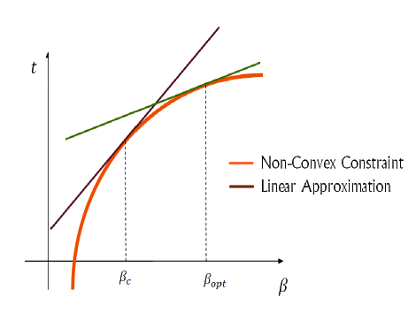
Figure 2: Linear approximation of $\log(\beta)$ around $\beta_{c}$.

The problem (41) can be efficiently solved by means of the interior-point based numerical methods. Once the optimal solution of this problem in the first iteration, denoted as $\mathbf{X}_{\rm opt}^{(1)}$, $\tau_{\rm opt}^{(1)}$ and $\beta_{\rm opt}^{(1)}$, is found, the algorithm proceeds to the second iteration by replacing the function $\log(\beta)$ by its linear approximation around $\beta_{\rm opt}^{(1)}$ found from the previous (first) iteration. Fig. 2 shows how $\log(\beta)$ is replaced by its linear approximation around $\beta_{c}$ where $\beta_{\rm opt}$ is the optimal value of $\beta$ obtained through solving (41) using such a linear approximation. In the second iteration, the resulting optimization problem has the same structure as the problem (41) in which $\beta_{c}$ has to be set to $\beta_{\rm opt}^{(1)}$ obtained from the first iteration. This process continues and every iteration is obtained by replacing $\log(\beta)$ at the iteration $k$ by its linearization of type (40) around $\beta_{\rm opt}^{(k-1)}$ found from the iteration $k-1$. The POTDC algorithm for solving the problem (39) is summarized in Algorithm 1.

Algorithm 1 The POTDC algorithm for solving the optimization problem (39)

  Initialize: Select an arbitrary $\beta_{c}$ from theinterval $[\lambda_{\min}({\bf B}_{1}^{-1}{\bf B}_{2}),\lambda_{\max}({\bf B}_{1}^{-1}{\bf B}_{2})]$, set the counter $k$ to be equal to $1$ and choose an accuracy parameter $\epsilon$.

  while The difference between the values of the objective function in two consecutive iterations is larger than $\epsilon$. do

     Use the linearization of type (40) and solve the following optimization problem

$$\max\limits_{\bf X,\tau,\beta}\!\!\! \!\!\!\log({\rm tr}({\bf A}_{1}\cdot{\bf X}))+\log(\tau)-t$$ (42)

$$\!\!\!{\rm tr}({\bf B}_{1}\cdot{\bf X})=1$$

$$\!\!\!{\rm tr}({\bf A}_{2}\cdot{\bf X})=\tau\$$

$$\!\!\!{\rm tr}({\bf B}_{2}\cdot{\bf X})=\beta$$

$$\!\!\!\log(\beta_{c})+\frac{1}{\beta_{c}}(\beta-\beta_{c})\leq t$$

$$\!\!\!{\bf X}\succeq{\bf 0}.$$

to obtain ${\bf X}_{\rm opt}^{(k)}$, $\tau_{\rm opt}^{(k)}$, and $\beta_{\rm opt}^{(k)}$.

     $k=k+1$

     Set ${\bf X}_{\rm opt}:={\bf X}_{\rm opt}^{(k)}$, and $\beta_{c}:=\beta_{\rm opt}^{(k)}$.

  end while

  Output: ${\bf X}_{\rm opt}$.

The following two lemmas regarding the proposed POTDC algorithm are of interest. First, the termination condition in the POTDC algorithm is guaranteed to be satisfied due to the following lemma which states that by choosing $\beta_{c}$ in the above proposed manner, the optimal values of the objective function of (41) for ${\bf X}_{\rm opt}^{(k)}$, $\tau_{\rm opt}^{(k)}$, and $\beta_{\rm opt}^{(k)}$ are non-decreasing.

Lemma 1: The optimal values of the objective function of the optimization problem (41) obtained over the iterations of the POTDC algorithm are non-decreasing.

Proof:

Considering the linearized problem (41) in the iteration $k+1$, it is easy to verify that ${\bf X}_{\rm opt}^{(k)}$, $\tau_{\rm opt}^{(k)}$, and $\beta_{\rm opt}^{(k)}$ give a feasible point for this problem. Therefore, it can be concluded that the optimal value at the iteration $k+1$ must be greater than or equal to the optimal value in the iteration $k$ which completes the proof. ∎

Second, it is guaranteed that the solution obtained using the POTDC algorithm is optimal due to the following lemma.

Lemma 2: The solution obtained using the POTDC algorithm satisfies the Karush -Kuhn -Tucker (KKT) conditions.

Proof:

This lemma follows straightforwardly from a similar proposition in [31]. ∎

As soon as the solution of the relaxed problem (39) is found, the solution of the original problem (35), which is equivalent to the solution of the sum-rate maximization problem (34), can be found using one of the existing methods for extracting a rank one solution. Among the existing methods are the ones based on solving the dual problem [28], which exploits the fact that the original problem (35) with only two constraints is strictly feasible and has zero duality gap; the algebraic technique of [30]; and the rank reduction-based technique of [29] which is also applicable for the problems with three constrains. Although the solution of (39) is guaranteed to be optimal, it is still left to show that this solution is also globally optimal.

V An Upper-Bound for the Optimal Value

Through extensive simulations we have observed that regardless of the initial value chosen for $\beta_{c}$ in the first iteration of the POTDC algorithm, the proposed iterative method always converges to the global optimum of the problem (39). However, since the original problem is not convex, this can not be easily verified analytically. A comparison between the optimal value obtained by using the proposed iterative method and also the global optimal value can be, however, done by developing a tight upper-bound for the optimal value of the problem and comparing the solution to such an upper-bound. Thus, in this section, we find such an upper-bound for the optimal value of the optimization problem (35). For this goal, we first consider the following lemma which gives an upper-bound for the optimal value of the variable $\beta$ in the problem (38). This lemma will further be used for obtaining the desired upper-bound for our problem.

Lemma 3: The optimal value of the variable $\beta$ in (39), denoted as $\beta_{\rm opt}$ is upper-bounded by $e^{(q^{\star}-p^{\star})}$, where $p^{\star}$ is the value of the objective function in the problem (39) corresponding to any arbitrary feasible point and $q^{\star}$ is the solution of the following convex optimization problem

$$q^{\star}=\mathop{\max}\limits_{\bf X,\tau,\beta}\!\!\! \!\!\!\log({\rm tr}({\bf A}_{1}\cdot{\bf X}))+\log(\tau)$$ (43)

$$\!\!\!{\rm tr}({\bf B}_{1}\cdot{\bf X})=1$$

$$\!\!\!{\rm tr}({\bf A}_{2}\cdot{\bf X})=\tau$$

$$\!\!\!{\bf X}\succeq{\bf 0}.$$

Proof:

First note that since $p^{\star}$ is the value of the objective function in the problem (39) corresponding to an arbitrary feasible point, it must be less than or equal to the optimal value of problem (39). By fixing the variable $\beta$ to $\beta_{\rm opt}$ in the optimization problem (39), the optimal value of the objective function does not change. Moreover, in the aforementioned case when $\beta$ has been fixed to $\beta_{\rm opt}$, dropping the constraint ${\rm tr}({\bf B}_{2}\cdot{\bf X})=\beta_{\rm opt}$ in that problem leads to the following optimization problem

$$\max\limits_{\bf X,\tau,\beta}\!\!\! \!\!\!\log({\rm tr}({\bf A}_{1}\cdot{\bf X}))+\log(\tau)-\log(\beta_{\rm opt})$$ (44)

$$\!\!\!{\rm tr}({\bf B}_{1}\cdot{\bf X})=1$$

$$\!\!\!{\rm tr}({\bf A}_{2}\cdot{\bf X})=\tau$$

$$\!\!\!{\bf X}\succeq{\bf 0}.$$

Noticing that the feasible set of the optimization problem (39) is a subset of the feasible set of the newly introduced optimization problem (44), it is straightforward to conclude that the optimal value of the problem (44) is bigger than or equal to the optimal value of the problem (39) and as a result it is greater than or equal to $p^{\star}$. Using (43), the optimal value of the optimization problem (44) can be expressed as $q^{\star}-\log(\beta_{\rm opt})$ which is bigger than or equal to $p^{\star}$ and, therefore, $\beta_{\rm opt}\leq e^{(q^{\star}-p^{\star})}$ which completes the proof. ∎

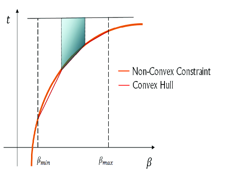
Figure 3: Feasible region of the constraint $\log(\beta)\leq t$ and the convex hull in each sub-division.

Note that as mentioned earlier, $p^{\star}$ is the objective value of the problem (39) that corresponds to an arbitrary feasible point. In order to obtain the tightest possible upper-bound for $\beta_{\rm opt}$, we choose $p^{\star}$ to be the largest possible value that we already know. A suitable choice for $p^{\star}$ is then the one which is obtained using the POTDC algorithm. In other words, we choose $p^{\star}$ as the corresponding objective value of the problem (39) at the optimal point which is resulted from the POTDC algorithm. Thus, we have obtained an upper-bound for $\beta_{\rm opt}$ which makes it further possible to develop an upper-bound for the optimal value of the optimization problem (39). To this end, we consider the only non-convex constraint of this problem, i.e., $\log(\beta)\leq t$. Fig. 3 illustrates a subset of the feasible region corresponding to the non-convex constraint $\log(\beta)\leq t$ where $\beta_{\min}$ equals $\lambda_{\min}(\mathbf{B}_{1}^{-1}\mathbf{B}_{2})$, i.e., the smallest value of $\beta$ for which the problem (39) is feasible, and $\beta_{\rm max}$ is the upper-bound for the optimal value $\beta_{\rm opt}$ given by Lemma 3. For obtaining an upper-bound for the optimal value of the problem (39), we divide the interval $[\beta_{\rm min},\beta_{\rm max}]$ into $N$ sections as it is shown in Fig. 3. Then, each section is considered separately. In each such section, the corresponding non-convex feasible set is replaced by its convex-hull and each corresponding optimization problem is solved separately as well. The maximum optimal value of such $N$ convex optimization problems is then the upper-bound. Indeed, solving the resulting $N$ convex optimization problems and choosing the maximum optimum value among them is equivalent to replacing the constraint $\log(\beta)\leq t$ with the feasible set which is described by the region above the thin line in Fig. 3. The upper-bound becomes more and more accurate when the number of the intervals, i.e., $N$ increases.

VI Semi-Algebraic Solution via Generalized Eigenvectors (RAGES)

In this section we present RAGES as an alternative solution to the sum-rate maximization problem (34) which is based on generalized eigenvectors. It requires a different parameterization than the one used in the POTDC algorithm and in some cases it is more efficient.

VI-A Basic Approach: Generalized Eigenvectors

To derive the link between (34) and generalized eigenvectors we start with the necessary condition for optimality that the gradient of (34) vanishes. Therefore, if we find all vectors ${\bf g}$ for which the gradient of the objective functions is zero, the global optimum must be one of them. By using the product rule and the chain rule of differentiation, the condition of zero gradient can be expressed as [25]

$$\frac{\tilde{P}_{R,2}}{\tilde{P}_{N,1}\cdot\tilde{P}_{N,2}}\cdot{\bf A}_{1}\cdot{\bf g}+\frac{\tilde{P}_{R,1}}{\tilde{P}_{N,1}\cdot\tilde{P}_{N,2}}\cdot{\bf A}_{2}\cdot{\bf g}$$

$$=\frac{\tilde{P}_{R,1}\cdot\tilde{P}_{R,2}}{\tilde{P}_{N,1}^{2}\cdot\tilde{P}_{N,2}}\cdot{\bf B}_{1}\cdot{\bf g}+\frac{\tilde{P}_{R,1}\cdot\tilde{P}_{R,2}}{\tilde{P}_{N,1}\cdot\tilde{P}_{N,2}^{2}}\cdot{\bf B}_{2}\cdot{\bf g}.$$ (45)

Rearranging (45) we obtain

$$\left({\bf A}_{1}+\rho_{\rm sig}\cdot{\bf A}_{2}\right)\cdot{\bf g}=\frac{\tilde{P}_{R,1}}{\tilde{P}_{N,1}}\cdot\left({\bf B}_{1}+\rho_{\rm noi}\cdot{\bf B}_{2}\right)\cdot{\bf g}$$ (46)

where $\rho_{\rm sig}$ and $\rho_{\rm noi}$ are defined via

$$\rho_{\rm sig}=\frac{\tilde{P}_{R,1}}{\tilde{P}_{R,2}}\quad\mbox{and}\quad\rho_{\rm noi}=\frac{\tilde{P}_{N,1}}{\tilde{P}_{N,2}}.$$ (47)

It follows from (46) that the optimal ${\bf g}$ must be a generalized eigenvector of the pair of matrices $\left({\bf A}_{1}+\rho_{\rm sig}\cdot{\bf A}_{2}\right)$ and $\left({\bf B}_{1}+\rho_{\rm noi}\cdot{\bf B}_{2}\right)$. Moreover, the corresponding generalized eigenvalue is given by ${\tilde{P}_{R,1}}/{\tilde{P}_{N,1}}$ which is logarithmically proportional to the rate of the terminal one $r_{1}$. Unfortunately, the matrices $\left({\bf A}_{1}+\rho_{\rm sig}\cdot{\bf A}_{2}\right)$ and $\left({\bf B}_{1}+\rho_{\rm noi}\cdot{\bf B}_{2}\right)$ contain the parameters $\rho_{\rm sig}$ and $\rho_{\rm noi}$ which also depend on ${\bf g}$ and are hence not known in advance. Therefore, we still need to optimize over these two parameters. However, compared to the original problem of finding a complex-valued $M_{R}\times M_{R}$ matrix, optimizing over the two real-valued scalar parameters is already significantly simpler. The following subsections show how to simplify this 2-D search even further.

VI-B Bounds on the parameters $\rho_{\rm sig}$ and $\rho_{\rm noi}$

Since both parameters $\rho_{\rm sig}$ and $\rho_{\rm noi}$ have a physical interpretation, the lower and upper-bounds for them can be easily found. Such bounds are useful since they limit the search space that has to be tested. For instance, $\rho_{\rm noi}$ can be expanded into

$$\rho_{\rm noi}=\frac{\tilde{P}_{N,1}}{\tilde{P}_{N,2}}=\frac{{\bf g}^{H}\cdot{\bf J}_{1}\cdot{\bf g}+P_{N,1}}{{\bf g}^{H}\cdot{\bf J}_{2}\cdot{\bf g}+P_{N,2}}.$$ (48)

The quadratic forms can be bounded by using the fact that for any Hermitian matrix ${\bf R}$ we have

$$\lambda_{\min}({\bf R})\cdot\|{\bf g}\|_{2}^{2}\leq{\bf g}^{H}\cdot{\bf R}\cdot{\bf g}\leq\lambda_{\max}({\bf R})\cdot\|{\bf g}\|_{2}^{2}$$ (49)

where $\lambda_{\min}({\bf R})$ and $\lambda_{\max}({\bf R})$ are the smallest and the largest eigenvalues of ${\bf R}$, respectively. It follows from (26) that

$$\lambda_{\min}({\bf J}_{1})=0\quad{\rm and}\quad\lambda_{\max}({\bf J}_{1})=\lambda_{\max}({\bf R}_{N,R})\cdot(\alpha_{i}^{(b)})^{2}$$ (50)

where $\alpha_{i}^{(b)}$ is a short hand notation for $\|{\bf h}_{i}^{(b)}\|_{2}$. Furthermore, in general the following inequity holds

$$\lambda_{\max}({\bf R}_{N,R})\leq P_{N,R}\cdot M_{R}$$ (51)

which for the case of white noise at the relay boils down to the following tighter condition $\lambda_{\max}({\bf R}_{N,R})=P_{N,R}$.

The relations (50) and (51) can be used to bound (48). Specifically, an upper-bound for $\rho_{\rm noi}$ can be found by upper-bounding the enumerator and lower-bounding the denominator, while the lower-bound can be found by lower-bounding the enumerator and upper-bounding the denominator. This yields

$$\rho_{\rm noi} \leq\frac{P_{N,R}}{P_{N,2}}\cdot M_{R}\cdot(\alpha_{1}^{(b)})^{2}\cdot\gamma^{2}+\frac{P_{N,1}}{P_{N,2}}$$ (52)

$$\rho_{\rm noi} \geq\left(\frac{P_{N,R}}{P_{N,1}}\cdot M_{R}\cdot(\alpha_{2}^{(b)})^{2}\cdot\gamma^{2}+\frac{P_{N,2}}{P_{N,1}}\right)^{-1}$$ (53)

where $\gamma^{2}=\|{\bf g}\|_{2}^{2}$ and $M_{R}$ can be dropped if the noise at the relay is white. However, an upper-bound for $\gamma^{2}$ is till needed. Due to the relay power constraint we have ${\bf g}^{H}\cdot{\bf Q}\cdot{\bf g}=P_{T,R}$. Using the latter condition, the following bound can be derived $\gamma^{2}\leq P_{T,R}/\lambda_{\min}({\bf Q})$. However, it is easy to check that this bound is very loose since for white noise at the relay we have $\lambda_{\min}({\bf Q})=P_{N,R}$ and for arbitrary relay noise covariance matrices no lower-bound exists (the infimum over $\lambda_{\min}$ is zero). This bound is so loose because it is extremely pessimistic: it measures the norm of ${\bf g}$ in the case when only noise is amplified and no power is put on the eigenvalues related to the signals of interest. However, such a case is practically irrelevant since it corresponds to a sum-rate equal to zero. Therefore, we propose to replace $\gamma^{2}$ in (52) and (53) by

$$\gamma^{2}:=\frac{(\alpha_{1}^{(f)})^{2}\cdot(\alpha_{2}^{(f)})^{2}\cdot P_{T,1}\cdot P_{T,2}}{(\alpha_{1}^{(f)})^{2}\cdot P_{T,1}+(\alpha_{2}^{(f)})^{2}\cdot P_{T,2}}.$$ (54)

In a similar manner, $\rho_{\rm sig}$ can be bounded. In this case, the enumerator and the denominator have the additional terms $P_{T,2}\cdot{\bf g}^{H}\cdot{\bf K}_{2,1}\cdot{\bf g}$ and $P_{T,1}\cdot{\bf g}^{H}\cdot{\bf K}_{1,2}\cdot{\bf g}$, respectively. A pessimistic (loose) bound is obtained by bounding these two terms independently, i.e., $0\leq{\bf g}^{H}\cdot{\bf K}_{2,1}\cdot{\bf g}\leq\gamma^{2}\cdot(\alpha_{2}^{(f)})^{2}\cdot(\alpha_{1}^{(b)})^{2}$ and $0\leq{\bf g}^{H}\cdot{\bf K}_{1,2}\cdot{\bf g}\leq\gamma^{2}\cdot(\alpha_{1}^{(f)})^{2}\cdot(\alpha_{2}^{(b)})^{2}$. This yields

$$\rho_{\rm sig} \leq\frac{P_{T,2}}{P_{N,2}}\cdot(\alpha_{2}^{(f)})^{2}\cdot(\alpha_{1}^{(b)})^{2}\cdot\gamma^{2}+\frac{P_{N,R}}{P_{N,2}}\cdot M_{R}\cdot(\alpha_{1}^{(b)})^{2}\cdot\gamma^{2}+\frac{P_{N,1}}{P_{N,2}}$$ (55)

$$\rho_{\rm sig} \geq\left(\frac{P_{T,1}}{P_{N,1}}\cdot(\alpha_{1}^{(f)})^{2}\cdot(\alpha_{2}^{(b)})^{2}\cdot\gamma^{2}+\frac{P_{N,R}}{P_{N,1}}\cdot M_{R}\cdot(\alpha_{2}^{(b)})^{2}\cdot\gamma^{2}+\frac{P_{N,2}}{P_{N,1}}\right)^{-1}.$$ (56)

Again, these bounds are pessimistic since they assume that there exists an optimal relay strategy for which $P_{R,1}=P_{T,2}\cdot(\alpha_{2}^{(f)})^{2}\cdot(\alpha_{1}^{(b)})^{2}\cdot\gamma^{2}$ but $P_{R,2}=0$, i.e., the rate of the second terminal is equal to zero. However, it is typically sum-rate optimal to have significantly more balanced rates between the two users. In fact, for the “symmetric” scenario when $P_{T,1}=P_{T,2}$, ${\bf h}_{i}^{(f)}={\bf h}_{i}^{(b)}$, $i=1,2$, and $\alpha_{1}^{(f)}=\alpha_{2}^{(f)}$, we always have $P_{R,1}=P_{R,2}$ at the optimal point. Therefore, these bounds can be further tightened if a priori knowledge about the scenario is available.

VI-C Efficient 2-D and 1-D Search

Once the search space for $\rho_{\rm sig}$ and $\rho_{\rm noi}$ has been fixed, we can find the maximum via optimization over these two parameters using a 2-D search. In general, a 2-D exhaustive search can be computationally demanding, i.e., the complexity will be higher than that of the POTDC algorithm. However, as we show in the sequel, for the problem at hand, this search can be implemented efficiently. These efficient implementations are, however, heuristic since they rely on properties of the objective functions that are apparent by visual inspection. As we will see in simulations, the resulting RAGES algorithm performs as well as the rigorous POTDC algorithm in practice.

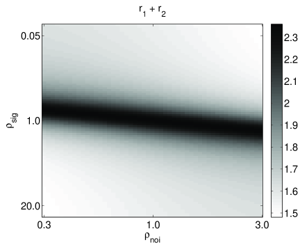
Figure 4: Sum-rate $r_{1}+r_{2}$ versus $\rho_{\rm sig}$ and $\rho_{\rm noi}$ for $M_{R}=6$, $P_{T,1}=P_{T,2}=P_{T,R}=1$, $P_{N,1}=P_{N,2}=P_{N,R}=0.1$.

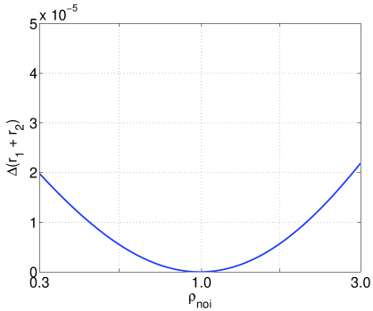
Figure 5: Relative change in sum-rate $r_{1}+r_{2}$ versus $\rho_{\rm noi}$: optimizing over $\rho_{\rm sig}$ for every choice of $\rho_{\rm noi}$. The same data set as in Fig. 4 is used.

Fig. 4 demonstrates a typical example of the sum-rate $r_{1}+r_{2}$ as a function of $\rho_{\rm sig}$ and $\rho_{\rm noi}$. For this example we have chosen $M_{R}=6$, $P_{T,1}=P_{T,2}=P_{T,R}=1$, $P_{N,1}=P_{N,2}=P_{N,R}=0.1$ and we have drawn the channel vectors from an uncorrelated Rayleigh fading distribution assuming reciprocity. By visual inspection, this sample objective function shows two interesting properties. First, it is a quasi-convex function with respect to the parameters $\rho_{\rm noi}$ and $\rho_{\rm sig}$ which allows for efficient (quasi-convex) optimization tools for finding its maximum. Albeit this property is only demonstrated for one example here, it has been always present in our numerical evaluations even when largely varying all system parameters. Secondly, for every value of $\rho_{\rm sig}$ the corresponding maximization over $\rho_{\rm noi}$ yields one maximal value which depends on $\rho_{\rm noi}$ only very weakly. This is illustrated by Fig. 5 which displays the relative change of the objective function $r_{1}+r_{2}$ for different choices of $\rho_{\rm noi}$, each time optimizing it over $\rho_{\rm sig}$. The displayed values represent the relative decrease of the objective functions compared to the global optimum, i.e., for the worst choice of $\rho_{\rm noi}$, the achieved sum-rate is about $2\cdot 10^{-5}=0.002$ % lower than for the best choice of $\rho_{\rm noi}$. Consequently, the 2-D search over $\rho_{\rm sig}$ and $\rho_{\rm noi}$ can be replaced essentially without any loss by a 1-D search over $\rho_{\rm sig}$ only for one fixed value of $\rho_{\rm noi}$ (e.g., the geometric mean of the upper and the lower-bound).

In addition, instead of performing the search directly over the original objective function $r_{1}+r_{2}$, we can find an even simpler objective functions by using the physical meaning of our two search parameters. To this end, let us introduce a new parameter $\hat{\rho}_{\rm sig}$ as a function of $\bf g$ as follows

$$\hat{\rho}_{\rm sig}({\bf g})=\frac{{\bf g}^{H}\cdot{\bf A}_{1}\cdot{\bf g}}{{\bf g}^{H}\cdot{\bf A}_{2}\cdot{\bf g}}.$$ (57)

Here ${\bf g}$ is the relay weight vector at the current search point ($\rho_{\rm sig},\rho_{\rm noi}$). Then we know that in the optimal point ${\bf g}_{\rm opt}$, we have $\hat{\rho}_{\rm sig}({\bf g}_{\rm opt})={\rho}_{\rm sig}$. This can be used to construct a new objective function

$$A_{\rm sig}(\rho_{\rm sig},\rho_{\rm noi})=\hat{\rho}_{\rm sig}({\bf g}_{\rm opt})-{\rho}_{\rm sig}$$ (58)

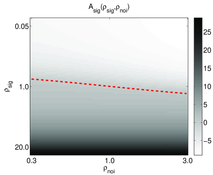
Figure 6: Objective function $A_{{\rm sig}}(\rho_{\rm sig},\rho_{\rm noi})$. The same data set as in Fig. 4 is used. The red dashed line indicates the points where $A_{{\rm sig}}(\rho_{\rm sig},\rho_{\rm noi})=0$.

Using the same data set as before, we display the corresponding shape of $A_{\rm sig}(\rho_{\rm sig},\rho_{\rm noi})$ in Fig. 6. The red dashed line indicates the set of points where $A_{\rm sig}(\rho_{\rm sig},\rho_{\rm noi})=0$. It can be observed that for every value of $\rho_{\rm noi}$, $A_{\rm sig}(\rho_{\rm sig},\rho_{\rm noi})$ is a monotonic function in $\rho_{\rm sig}$. Therefore, the bisection method can be used to find a zero crossing in $\rho_{\rm sig}$ which coincides with the sum-rate-optimal $\rho_{\rm sig}$ for a given $\rho_{\rm noi}$.

VI-D Summary

In summary, it can be concluded that the RAGES approach simplifies the optimization over a complex-valued $M_{R}\times M_{R}$ matrix into the optimization over two real-valued parameters which both have a physical interpretation. Even more, the 2-D search can be simplified into a 1-D search by fixing one of the parameters. The loss incurred to this step is typically small. In the example provided above, it is only 0.002 %, but even varying the system parameters largely and using many random trials we never found a relative difference higher than a few percents.

Moreover, the 1-D search can be efficiently implemented by exploiting the quasi-convexity of $r_{1}+r_{2}$ or the monotonicity of $A_{\rm sig}$ (e.g., using the bisection method). Again, these properties are only demonstrated by examples but we have observed in all our simulations that the resulting algorithm yields a sum-rate very close to the optimum found by the exact solution and its upper-bound described before. This comparison is further illustrated in next section via numerical simulations.

Comparing the POTDC and RAGES approaches, it is noticeable that the POTDC approach is absolutely rigorous, while the RAGES approach is at some points heuristic. The complexity of solving the proposed sum-rate maximization problem for two-way AF MIMO relaying using the POTDC algorithm is the same as the complexity of solving the semi-definite programming problem (39) and iterating over a single parameter $\beta$. The typical number of iterations is 4-7. Alternatively, the complexity of solving the same problem using the RAGES approach is equivalent to the complexity of finding the dominant generalized eigenvector, which has to be performed for each combination of the parameters $\rho_{\rm sig}$ and $\rho_{\rm noi}$. Since, as has been shown, the search over one parameter only is sufficient, the complexity of the RAGES approach is typically lower than that of the POTDC algorithm, especially for the 1-D RAGES.

VII Simulation Results

In this section, we evaluate the performance of the new proposed methods via numerical simulations. Consider a communication system consisting of two single-antenna terminals and an AF MIMO relay with $M_{R}$ antenna elements. The communication between the terminals is bidirectional, i.e., it is performed based on the two-way relaying scheme. It is assumed that perfect channel knowledge is available at the terminals and at the relay, while the terminals use only effective channels (scalars), but the relay needs full channel vectors. The relay estimates the corresponding channel coefficients between the relay antenna elements and the terminals based on the pilots which are transmitted from the terminals. Then based on these channel vectors, the relay computes the relay amplification matrix $\mathbf{G}$ and then uses it for forwarding the pilot signals to the terminals. After receiving the forwarded pilot signals from the relay via the effective channels, the terminals can estimate the effective channels using a suitable pilot-based channel estimation scheme, e.g., the LS.

The noise powers of the relays and the terminals $P_{N,R}$, $P_{N,1}$ and $P_{N,2}$ are assumed to be equal to $\sigma^{2}$. Uncorrelated Rayleigh fading channels are considered and it is assumed that reciprocity holds, i.e., ${\bf h}_{i}^{(f)}={\bf h}_{i}^{(b)}$ for $i=1,2$. The relay is assumed to be located on a line of unit length which connects the terminals to each other and the variances of the channel coefficients between terminal $i,i=1,2$ and the relay antenna elements are all assumed to be proportional to $1/d_{i}^{\nu}$, where $d_{i}\in(0,1)$ is the normalized distance between the relay and the terminal $i$ and $\nu$ is the path-loss exponent which is assumed to be equal to $3$ throughout the simulations. For obtaining each simulated point, $100$ independent simulation runs are used unless otherwise is specified.

In order to design the relay amplification matrix $\mathbf{G}$, five different methods are considered including the proposed POTDC, 2-D RAGES and 1-D RAGES algorithms, the algebraic norm-maximizing (ANOMAX) transmit strategy of [32] and the discrete Fourier transform (DFT) method that chooses the relay precoding matrix as a scaled DFT matrix. Note that the ANOMAX strategy provides a closed-form solution for the problem. Also note that for the DFT method no channel knowledge is needed. Thus, the DFT method serves as a benchmark for evaluating the gain achieved by using channel knowledge. The upper-bound is also shown in all simulations. For obtaining the upper-bound, the interval $[\beta_{\min},\beta_{\max}]$ is divided in $30$ segments. In addition, the proposed techniques are compared to the SNR-balancing technique of [33] for the relevant to the later technique scenario when multiple single-antenna relay nodes are used.

VII-A Example 1: Symmetric Channel Conditions

In our first example, we consider the case when the channels between the relay antenna elements and both terminals have the same channel quality. More specifically, it is assumed that the relay is located in the middle of the connecting line between the terminals and the transmit power of the terminals $P_{T,1}$ and $P_{T,2}$ and the total transmit power of the MIMO relay $P_{T,R}$ are all assumed to be equal to $1$.

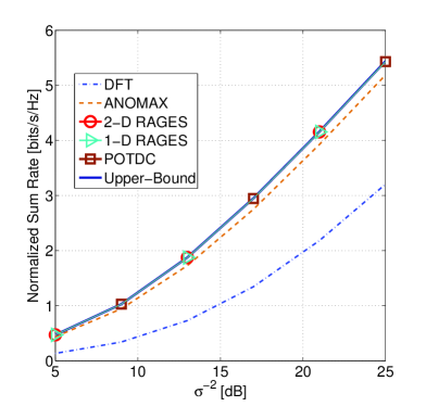
Figure 7: Sum-rate versus $\sigma^{-2}$ for $M_{R}=3$ antennas. The case of symmetric channel conditions.

Fig. 7 shows the sum-rate achieved by different aforementioned methods versus $\sigma^{-2}$ for the case of $M_{R}=3$. It can be seen in this figure that the performance of the proposed methods coincides with the upper-bound. Thus, the methods perform optimally in terms of providing the maximum sum-rate. The ANOMAX technique performs close to the optimal, while the DFT method gives a significantly lower sum-rate.

VII-B Example 2: Asymmetric Channel Conditions

In the second example, we consider the case when the channels between the relay antenna elements and the second terminal have better channel quality than the channels between the relay antenna elements and the first terminal and, and evaluate the effect of the relay location on the achievable sum-rate. Particularly, we consider the case when the distance between the relay and the second terminal, $d_{2}$, is less than or equal to the distance between the relay and the first terminal, $d_{1}$. The total transmit power of the terminals, i.e., $P_{T,1}$ and $P_{T,2}$ and the total transmit power of the MIMO relay $P_{T,R}$ all are assumed to be equal to $1$ and the noise power in the relays and the terminals all are assumed to be equal to $1$.

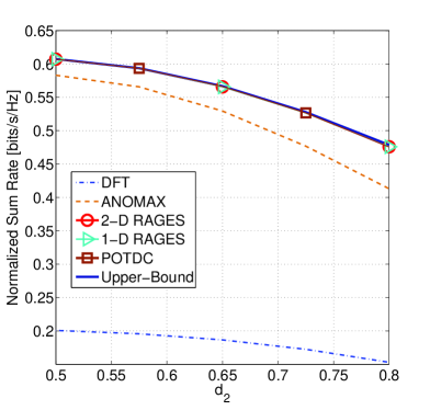
Figure 8: Sum-rate versus the distance between the relay and the second terminal $d_{2}$ for $M_{R}=3$ antennas. The case of asymmetric channel conditions.

Fig. 8 shows the sum-rate achieved in this scenario by different aforementioned methods versus the distance between the relay and the second terminal denoted as $d_{2}$, for the case of $M_{R}=3$. It can be seen in this figure that the proposed methods perform optimally, while the performance (sum-rate) of ANOMAX is slightly worse.

As mentioned earlier, it is guaranteed that the POTDC algorithm converges to at least a local maximum of the sum-rate maximization problem. However, our extensive simulation results confirm that the POTDC algorithm converges to the global maximum of the problem in all simulation runs. Indeed, the performance of the POTDC algorithm coincides with the upper-bound. Moreover, the 2-D RAGES and 1-D RAGES are, in fact, globally optimal, too. The ANOMAX and DFT methods, however, do not achieve the maximum sum-rate. The loss in sum-rate related to the DFT method is quite significant while the loss in sum-rate related to the ANOMAX method grows from small in the case of symmetric channel conditions to significant in the case of asymmetric channel conditions. Although ANOMAX enjoys a closed-form solution and it is even applicable in the case when terminals have multiple antennas, it is not a good substitute for the proposed methods for the sum-rate maximization goal, because of this significant gap in performance in the asymmetric case.

VII-C Example 3: Effect of The Number of Relay Antenna Elements

In this example, we consider the effect of the number of relay antenna elements $M_{R}$ on the achievable sum-rate for the aforementioned methods. The powers assigned to the first and the second terminals as well as to the relay are all equal to 1. The relay is assumed to be located at the distance of $1/4$ from the second user. Moreover, the noise powers at the terminals and at the relay antenna elements are all assumed to be equal to $1$. For obtaining each simulated point in this simulation example, $200$ independent simulation runs are used.

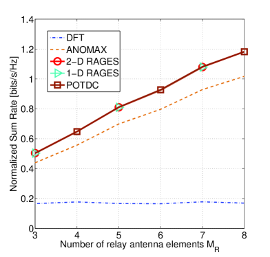
Figure 9: Sum-rate versus the number of the relay antenna elements $M_{R}$. The case of asymmetric channel conditions.

Fig. 9 depicts the sum-rates achieved by different methods versus the number of relay antenna elements $M_{R}$. As it is expected, by increasing $M_{R}$ (thus, increasing the number of degrees of freedom), the sum-rate increases. For the DFT method, the sum rate does not increase with an increase in the number of the relay antennas because of the lack of channel knowledge for this method. The proposed methods achieve higher sum-rate compared to ANOMAX.

VII-D Example 4: Performance Comparison for the Scenario of Two-Way Relaying via Multiple Single-Antenna Relays

In our last example, we compare the proposed methods with the SNR balancing-based approach of [33]. The method of [33] is developed for a two-way relaying system which consists of two single-antenna terminals and multiple single-antenna relay nodes. Subject to the constraint on the total transmit power of the relay nodes and the terminals, the method of [33] designs a beamforming vector for the relay nodes and the transmit powers of the terminals to maximize the minimum received SNR at the terminals. In order to make a fair comparison, we consider a diagonal structure for the relay amplification matrix $\mathbf{G}$ that corresponds to the special case of [33] when multiple single-antenna nodes are used for relaying. It is worth mentioning that for imposing such a diagonal structure for the relay amplification matrix $\mathbf{G}$ in POTDC and RAGES, the vector $\mathbf{g}_{M_{R}^{2}\times 1}={\rm vec}(\mathbf{G})$ is replaced with $\mathbf{g}_{M_{R}\times 1}={\rm diag}(\mathbf{G})$ and the matrices $\mathbf{A}_{i}$ and $\mathbf{B}_{i},i=1,2$ are replaced with new square matrices $\mathbf{\tilde{A}}_{i}$ and $\mathbf{\tilde{B}}_{i},i=1,2$ of size $M_{R}\times M_{R}$ such that $\mathbf{\tilde{A}}_{i}\ (m,n)=\mathbf{A}_{i}\ ((m-1)\cdot M_{R}+m,(n-1)\cdot M_{R}+n)$ and $\mathbf{\tilde{B}}_{i}\ (m,n)=\mathbf{B}_{i}\ ((m-1)\cdot M_{R}+m,(n-1)\cdot M_{R}+n),\ \ m,n=1,\cdots,M_{R}$. Moreover, we assume fixed transmit powers at the terminals and choose them to be equal to $1$. The total transmit power at the relay also equals $1$ and the relay is assumed to lie in the middle of the terminals. Fig. 10 shows the corresponding performance of the different methods. From this figure it can be observed that the proposed methods demonstrate a significantly better performance compared to the method of [33] as it may be expected.

VIII Conclusions and Discussions

We have shown that the sum-rate maximization problem in two-way AF MIMO relaying belongs to the class of DC programming problems. Although the typical approach for solving the DC programming problems is the branch-and-bound method, it does not have any polynomial time guarantees for its worst-case complexity. Therefore, we have developed in this paper two algorithms for finding the global maximum of the aforementioned problem with polynomial time worst-case complexity. The POTDC algorithm is based on a specific parameterization of the objective function, that is, the product of quadratic ratios, and then application of semi-definite programming (SDP) relaxation, linearization and iterative search over a single parameter. Its design is rigorous and is based on the recent advances in convex optimization. To the best of our knowledge, this is the first polynomial time algorithm for solving a class of DC programming problems rigorously. The RAGES algorithm is based on a different parameterization of the objective function and the generalized eigenvectors method, but may enjoy a lower computational complexity that makes it a valid alternative especially if 1-D search is used. The upper-bound for the solution of the problem is developed and it is demonstrated by simulations that both proposed method achieve the upper-bound and are, thus, globally optimal.

The proposed POTDC algorithm represents a general optimization technique applicable for solving a wide class of DC programming problems. Essentially, the optimization problems consisting of the maximization/minimization of a product of quadratic ratios can be handled using the proposed POTDC approach. Moreover, the POTDC algorithm can be used for solving the optimization problems containing in any of the constraints a difference of two quadratic forms. Some relatively straightforward modifications may, however, be required. For example, if the problem is to optimize a product of more than two quadratic ratios under a single quadratic (power) constraint, the number of constraints in the corresponding DC programming problem will be more than three. Thus, the result used in this paper that even after relaxing the rank-one constraint in the step of SDP relaxation, it is possible to find algebraically an exact rank-one solution based on the solution of the relaxed problem, does not hold any longer. Then, randomization procedures will have to be adopted to recover a rank-one solution from the solution of the relaxed problem. In this case, such solutions obviously may not be exact, but all the results related to the SDP relaxation will apply.

Other signal processing problems that can be addressed using the proposed POTDC approach are the general-rank robust adaptive beamformer with a positive semi-definite constraint [10], the dynamic spectrum management for digital subscriber lines [12], the problems of finding the weighted sum-rate point, the proportional-fairness operating point and the max-min optimal point for MISO interference channel [13], the problem of robust beamforming design for AF relay networks with multiple relay nodes and so on. The extensions of the POTDC approach to some of the aforementioned problem is an issue of future research.

\psfrag{AA}[cc][cc]{\Large{UT${}_{1}$}}\psfrag{BB}[cc][cc]{\Large{UT${}_{2}$}}\psfrag{C}[cc][cc]{\Large{RS}}\psfrag{hh}{\small$1$}\psfrag{kk}{\small$M_{R}$}\includegraphics[width=170.71652pt,height=99.58464pt,trim=34.1433pt 34.1433pt 34.1433pt 14.22636pt]{Fig1.eps}

Figure 1: Two-way relaying system model.

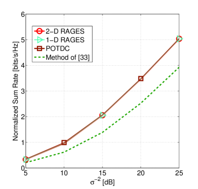
Figure 10: Sum-rate versus $\sigma^{-2}$ for $M_{R}=3$ antennas. The case of symmetric channel conditions.

References

- [1] B. Rankov and A. Wittneben, “Spectral efficient protocols for half-duplex fading relay channels,” IEEE Joulnal on Selected Areas in Communications, vol. 25, pp.379–389, Feb. 2007.
- [2] T. J. Oechterding, I. Bjelakovic, C. Schnurr, and H. Boche, “Broadcast capacity region of two-phase bidirectional relaying,” IEEE Trans. Information Theory, vol. 54, pp. 454–458, jan. 2008.
- [3] R. Ahlswede, N. Cai, S.-Y. R. Li, and R. W. Yeung, “Network information flow,” IEEE Trans. Information Thory, vol. 46, no. 4, pp. 1204–1216, Jul. 2000.
- [4] R. Zhang, Y.-C. Liang, C. C. Chai, and S. Cui, “Optimal beamforming for two-way multi-antenna relay channel with analogue network coding,” IEEE Journal on Selected Areas of Communications, vol. 27, no. 5, pp. 699–712, June 2009.
- [5] Y. Rong, X. Tang, and Y. Hua, “A unified framework for optimization linear non-regenerative multicarrier MIMO relay communication systems,” IEEE Trans. Signal Processing, vol. 57, pp. 4837–4852, Dec. 2009.
- [6] I. Hammerstrom, M. Kuhn, C. Esli, J. Zhao, A. Wittneben, and G. Bauch, “MIMO two-way relaying with transmit CSI at the relay,” in Proc. IEEE Signal Processing Advances in Wireless Communications, Helsinki, Finland, June 2007.
- [7] J. Joung and A. H. Sayed, “Multiuser two-way amplify-and-forward relay processing and power control methods for beamforming systems,” IEEE Trans. Signal Processing, vol. 58, pp. 1833–1846, Mar. 2010.
- [8] A. U T. Amah and A. Klein, “Pair-aware transceive beamforming for non-regenerative multi-user two-way relaying,” in Proc. IEEE Int. Conf. Acoustic, Speech, and Signal Processing, Dallas, TX, Mar. 2010.
- [9] H. H. Chen and A. B. Gershman, “Robust adaptive beamforming for general-rank signal models with positive semi-definite constraints,” in Proc. IEEE Int. Conf. Acoustic, Speech, and Signal Processing, Las Vegas, USA, Apr. 2008, pp. 2341–2344.
- [10] A. Khabbazibasmenj and S. A. Vorobyov “A computationally efficient robust adaptive beamforming for general-rank signal model with positive semi-definite constraint,” in Proc. Inter. Workshop Comp. Advances in Multi-Sensor Adaptive Processing, San Juan, Puerto Rico, Dec. 2011, accepted.
- [11] T. K. Phan, S. A. Vorobyov, C. Tellambura, and T. Le-Ngoc, “Power control for wireless cellular systems via D.C. programming,” in Proc. 14th IEEE Workshop Statistical Signal Processing, Madison, WI, USA, Aug. 2007, pp. 507–511.
- [12] Y. Xu, S. Panigrahi, and T. Le-Ngoc, “A concave minimization approach to dynamic spectrum management for digital subscriber lines,” in Proc. IEEE Inter, Conf. Communications Istambul, Turkey, Jun. 2006, pp. 84–89.
- [13] E. A. Jorswieck and E. G. Larsson, “Monotonic optimization framework for the two-user MISO interference channel,” IEEE Trans. Communications, vol. 58, pp. 2159–2168, July 2010.
- [14] P. C. Weeraddana, M. Codreanu, M. Latva-aho, and A. Ephremides, “Weighted sum-rate maximization for a set of intertering links via branch-and-bound,” IEEE Trans. Signal Processing, vol. 59, pp. 3977–3996, Aug. 2011.
- [15] R. Horst, P. M. Pardalos, and N. V. Thoai, Introduction to Global Optimization. Dordrecht, Netherlands: Kluwer Academic Publishers, 1995.
- [16] R. Horst and H. Tuy, Global Optimization: Deterministic Approaches. Springer, 1996.
- [17] H. Tuy, Convex Analysis and Global Optimization. Kluwer Academic Publishers, 1998.
- [18] A. Rubinov, H. Tuy, and H. Mays, “An algorithm for monotonic global optimization problems,” Optimization, vol. 49, pp. 205–221, 2001.
- [19] H. Tuy, F. Al-Khayyal, and P. T. Thach, Essays and Surveys in Global Pptimization. Springer US, 2005, ch. Monotonic, pp. 39–78.
- [20] S. A. Vorobyov, A. B. Gershman, and Z.-Q. Luo, “Robust adaptive beamforming using worst-case performance optimization: A solution to the signal mismatch problem,” IEEE Trans. Signal Processing, vol. 51, pp. 313–324, Feb. 2003.
- [21] N. D. Sidiropoulos, T. N. Davidson, and Z.-Q. Luo “Transmit beamforming for physical-layer multicasting,” IEEE Trans. Signal Processing, vol. 54, pp. 2239–2251, June 2006.
- [22] A. Beck and Y. Eldar, “Doubly constrained robust Capon beamformer with ellipsoidal uncertainty set,” IEEE Trans. Signal Processing, vol. 55, pp. 753–758, Jan. 2007.
- [23] A. De Maio, Y. Huang, D. P. Palomar, S. Zhang, and A. Farina, “Fractional QCQP with application in ML steering direction estimation for radar detection,” IEEE Trans. Signal Processing, vol. 59, pp. 172–185, Jan. 2011.
- [24] A. Khabbazibasmenj, S. A. Vorobyov, F. Roemer, and M. Haardt, “Sum-rate maximization in two-way MIMO relaying via polynomial time DC programming,” IEEE Int. Conf. Acoustic, Speech, and Signal Processing, Kyoto, Japan, Mar. 2012, submitted.
- [25] F. Roemer and M. Haardt, “Sum-rate maximization in two-way relaying systems with MIMO amplify and forward relays via generalized eigenvectors,” in Proc. 18-th European Sig. Proc. Conf., Aalborg, Denmark, Aug. 2010.
- [26] P. Vandewalle, J. Kovacevic, and M. Vetterli, “Reproducible research in signal processing,” IEEE Signal Process. Mag., vol. 26, no. 3, pp. 37–47, May 2009.
- [27] F. Roemer and M. Haardt, “Tensor-based channel estimation (TENCE) and iterative refinements for two-way relaying with multiple antennas and spatial reuse,” IEEE Trans. Signal Processing, vol. 58, no. 11, pp. 5720–5735, Nov. 2010.
- [28] A. Beck and Y. C. Eldar, “Strong duality in nonconvex quadratic optimization with two quadratic constraints,” SIAM J. Optimization, vol. 17, no. 3, pp. 844–860, Mar. 2006.
- [29] Y. Huang and D. P. Palomar, “Rank-constrained separable semidefinite programming with applications to optimal beamforming,” IEEE Trans. Signal Processing, vol. 58, pp. 664–678, Feb. 2010.
- [30] A. Khabbazibasmenj and S. A. Vorobyov and A. Hassanien, “Robust adaptive beamforming via estimating steering vector based on semidefinite relaxation,” in Proc. 44th Annual Asilomar Conf. Signals, Systems, and Computers, Pacific Grove, CA, USA, Nov. 2010, pp. 1102–1106.
- [31] A. Beck, A. Ben-Tal and L. Tetruashvili, “A sequential parametric convex approximation method with applications to nonconvex truss topology design problems,” Journal of Global Optimization, 47, no.1, pp. 29–51, 2010.
- [32] F. Roemer and M. Haardt, “Algebraic norm-maximizing (ANOMAX) transmit strategy for two-way relaying with MIMO amplify and forward relays,” IEEE Sig. Proc. Letters, vol. 16, no. 10, Oct. 2009.
- [33] S. Shahbazpanahi and M. Dong, “A semi-closed form solution to the SNR balancing problem of two-way relay network beamforming,” in Proc. IEEE Int. Conf. Acoustics, Speech, Signal Processing (ICASSP), Apr. 2010, pp. 2514-2517.
- [34] A. Goldsmith, Wireless Communications. Cambridge University Press, 2005.