Entanglement detection and quantum metrology by Raman photon diffraction imaging

Abstract

We show that far field diffraction image of spontaneously scattered Raman photons can be used for detection of spin entanglement and for metrology of fields gradients in cold atomic ensembles. For many-body states with small or maximum uncertainty in spin-excitation number, entanglement is simply witnessed by the presence of a sharp diffraction peak or dip. Gradient vector of external fields is measured by the displacement of a diffraction peak due to inhomogeneous spin precessions, which suggests a new possibility for precision measurement beyond the standard quantum limit without entanglement. Monitoring temporal decay of the diffraction peak can also realize non-demolition probe of temperature and collisional interactions in trapped cold atomic gases. The approach can be readily generalized to cold molecules, trapped ions, and solid state spin ensembles.

I Introduction

Cold atomic ensembles offer an ideal platform for the study of quantum many-body physics and for the implementation of quantum information processing Bloch_RMP . With entanglement speculated as a key phenomenon in these occasions, efficient approach to detect entanglement is crucial for understanding its profound roles Guhne_entanglementdetection . Spin of cold atoms is also widely used for precision measurement of external fields. A topic of current interest is quantum metrology which utilizes quantum properties and particularly entanglement in the probe system to reach measurement sensitivity beyond the standard quantum limit (SQL) Lloyd_metrology .

To address these outstanding demands in the exploration of quantum physics and quantum technology using cold atomic ensembles, the key is efficient access to the right piece of information in the spin subspace. An ideal interface between spin and photon is offered by the process of spontaneous Stokes scattering EIT ; DLCZ ; quantum_memory0 ; quantum_memory1 ; quantum_memory2 ; quantum_memory3 ; quantum_memory4 ; Pan_quantummemory ; dephaseinOL1 ; dephaseinOL2 : with a laser driving an ensemble of atoms in $\Lambda$-configuration, a collective spin-excitation can be spontaneously converted into a Stokes photon with phase and wavevector preserved. One may thus anticipate that photon diffraction pattern can provide information on collective spin properties. Earlier studies on the diffraction of collectively emitted photons have focused on the super-radiance phenomenon (i.e. induced directional coherent radiation) in very dense atomic ensembles Eberly_superradiance ; Haroche_superradiance ; Carmichael_superradiance , or in ensembles prepared with a single excitation Wstate ; Scully_singlephotonsuperradiance1 ; Scully_singlephotonsuperradiance2 ; Eberly_singlephotonsuperradiance ; Wstate2 .

In this paper, we show that the far field diffraction image of spontaneously emitted Raman photons can be used for detection of spin entanglement and for precision measurement of gradient vector of external fields in cold atomic ensembles. We find the strength of a sharp diffraction peak or dip measures spin pair-correlation sum and detects entanglement through pair-correlation sum rules we derive from optimal spin squeezing inequalities Sorensen_spinsqueezing ; Korbicz_spinsqueezing ; Toth_squeezing ; Duan2011 . For many-body states with small or maximum uncertainty in spin-excitation number, entanglement is simply witnessed by the presence of the peak or dip. Inhomogeneous spin precessions in a field gradient lead to displacement of the diffraction peak (dip), which can serve as a principle for vector metrology of fields gradients and for calibration of inhomogeneity in optical lattices. The gradiometer sensitivity can reach $1/N$ by using a spin-coherent-state of $N$ unentangled atoms as the probe, which suggests a new possibility for going beyond the SQL of $1/\sqrt{N}$ without entanglement fockstates1 ; fockstates2 ; HL1 ; HL2 . Motional dynamics leads to temporal decay of the diffraction peak which can be used for non-demolition probe of temperature and collisional interactions in trapped atomic gases.

Two remarkable features make this approach particularly suitable for ensembles with large number of atoms. First, regardless of the ensemble size, spin dephasing noise as a major error source only results in decay of the peak (dip) strength in a timescale equal to the dephasing time of a single spin. Second, the number of useful photons from a single copy of many-body state can be as large as its spin-excitation number for cold atomic ensembles which are typically dilute (i.e. interatomic distance comparable to or larger than optical wavelength). This approach complements existing optical methods for probing many-body quantum states Altman ; Eckert ; Bruun ; Vega ; Corcovilos ; Miyake ; Weitenberg , and is readily applicable in other systems including molecular ensembles, trapped ions and solid state spin ensembles.

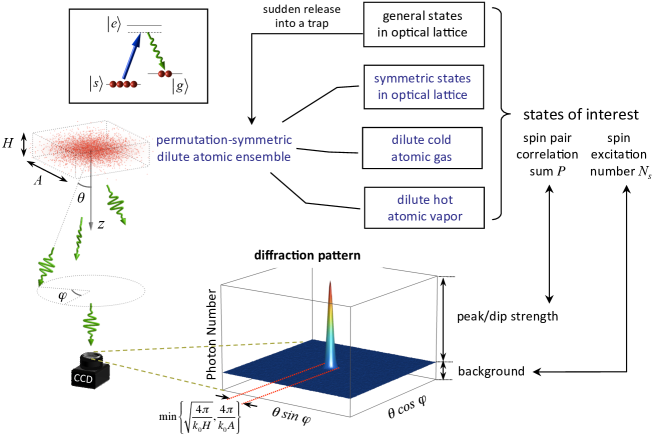
Figure 1: Far field diffraction image of Stokes photons from permutation-symmetric dilute ensembles. The pair-correlation sum $P$ in the many-atom state of interest manifests as a sharp diffraction peak (for $P>0$) or dip (for $P<0$) along the forward direction, with strength $\propto|P|$ and width inversely proportional to the ensemble size.

The rest of the paper is organized as follows. In section II, we analyze the the far field diffraction pattern of Raman photons and show how to extract the pair-correlation sum of atomic spins. In section III, we derive pair-correlation sum rules for detecting entanglement. In section IV, we analyze the time evolution of the diffraction pattern from dilute ensembles. In section V, we discuss the use of the diffraction pattern for precision measurement of field gradient and for non-demolition probe of atomic motion and temperature. Section VI is a brief summary to the paper. More supplementary details on the derivations are grouped in the Appendices.

II Diffraction Pattern of Stokes Photons

Consider an optically thin cold atomic ensemble with a $\Lambda$ level configuration where two atomic ground states $|g\rangle$ and $|s\rangle$ can be optically coupled to a common excited state $|e\rangle$ (Fig. 1 inset). The ensemble is driven by a laser with Rabi frequency $\Omega_{L}$, detuning $\Delta$ and wavevector $\mathbf{k}_{0}=k_{0}\hat{\mathbf{z}}$. We assume atomic motion can be taken as frozen in the duration of photon emission. With the laser coupling the $|s\rangle$ to $|e\rangle$ transition, an atom can go from state $|s\rangle$ to $|g\rangle$ by emitting a Stokes photon into the vacuum. When $\Delta$ is much larger than $\Omega_{L}$ and the excited state homogeneous line width $\Gamma_{0}$, $|e\rangle$ can be adiabatically eliminated, leading to the effective light-atom coupling in the electric-dipole and rotating wave approximation:

$$\hat{H} = \sum_{\mathbf{k}}\hbar\omega_{k}\hat{a}_{\mathbf{k}}^{\dagger}\hat{a}_{\mathbf{k}}+\sum_{j}E_{z}\hat{\sigma}_{j}^{z}$$ (1)

$$+\sum_{\mathbf{k}}g_{\mathbf{k}}\sum_{j}\mathrm{e}^{-i(\mathbf{k}-\mathbf{k}_{0})\cdot\mathbf{r}_{j}}\hat{\sigma}_{j}^{-}\hat{a}_{\mathbf{k}}^{\dagger}+\textrm{h.c.}.$$

Here $g_{\mathbf{k}}=\frac{\Omega_{L}}{2\Delta}\sqrt{\frac{2\pi\omega_{k}}{V}}\hat{\mathbf{e}}_{\mathbf{k}}\cdot\boldsymbol{\mu}$, $\hat{\mathbf{e}}_{\mathbf{k}}$ and $\boldsymbol{\mu}$ being respectively the unit polarization vector and the single atom dipole. $\hat{\sigma}_{j}^{-}\equiv|g\rangle_{j}\langle s|$ and $\hat{\sigma}_{j}^{z}\equiv|s\rangle_{j}\langle s|-|g\rangle_{j}\langle g|$. We assume anti-Stokes scattering is either forbidden by the polarization selection rule or suppressed by the much larger detuning when $E_{z}\gg\hbar\Delta$.

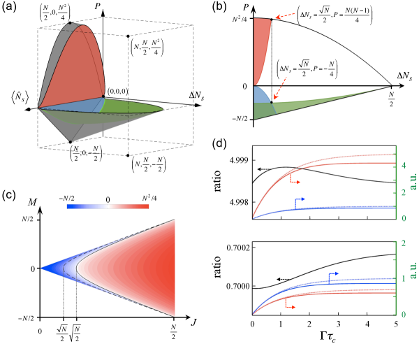
Figure 2: (a) Phase diagram in the parameter space $(\langle\hat{N}_{s}\rangle,\Delta N_{s},P)$. States in the surrounded region are all entangled ones. (b) A slice of (a) taken for $\langle\hat{N}_{s}\rangle=N/2$. The red, blue and green regions are entangled states violating inequalities (4a), (4b) and (4c) respectively. The grey surfaces in (a) and the black curves in (b) are boundaries between physical and unphysical regions. Positive and negative sections of $P$ axis use different linear scale. (c) Strength of the diffraction peak (red) or dip (blue) for eigenstates of total spin $\hat{J}^{2}$ and $\hat{J}_{z}$. Inequalities (4a) and (4b) are violated in the peak and dip regions respectively. States violating inequality (4c) form a subset of the dip region, to the left of the dashed curve. (d) Upper (lower): peak (dip) to background ratio as a function of the collection interval $\tau_{c}$ for a half-spin-excitation state with $P=2.5N$ ($P=-0.35N$), shown as the black curve. The calculation is for $N=4000$ atoms of a 2D Gaussian distribution with FWHM $A=100~{}\mu$m. Peak or dip (background) strength is evaluated at $\theta=0$ ($\theta=\frac{2\pi}{k_{0}A}$), shown by the blue (red) solid curve. Dashed curves are calculations with the multiple-light scattering and dipole-dipole interaction neglected.

Emission of a Stokes photon into mode $\mathbf{k}=(k,\theta,\varphi)$ is accompanied by the annihilation of a spin excitation by $\hat{J}^{-}(\Delta\mathbf{k})\equiv\sum_{j=1}^{N}\mathrm{e}^{-i\Delta\mathbf{k}\cdot\mathbf{r}_{j}}\hat{\sigma}_{j}^{-}$, $\Delta\mathbf{k}=\mathbf{k}-\mathbf{k}_{0}$. The angular distribution of the photon emission rate is given by $I(\theta,\varphi,t)=I_{s}(\theta)I_{c}(\theta,\varphi,t)$. $I_{s}$ is the single atom dipole emission pattern, a slow varying function of $\theta$. $I_{c}(\theta,\varphi,t)\equiv\textrm{Tr}[\hat{J}^{+}(\Delta\mathbf{k})\hat{J}^{-}(\Delta\mathbf{k})\rho(t)]$ is the collective factor where $\rho(t)$ is the atomic density matrix. At the initial time of photon emission,

$$I_{c}(\theta,\varphi,0) = \langle\hat{N}_{s}\rangle+\sum_{j\neq j^{\prime}}\mathrm{e}^{-i\Delta\mathbf{k}\cdot(\mathbf{r}_{j}-\mathbf{r}_{j^{\prime}})}\langle\hat{\sigma}_{j^{\prime}}^{+}\hat{\sigma}_{j}^{-}\rangle$$

$$= \langle\hat{N}_{s}\rangle-\frac{P}{N-1}+P\frac{|\langle\sum_{j}e^{-i\Delta\mathbf{k}\cdot\mathbf{r}_{j}}\rangle|^{2}}{N^{2}-N},$$

where $\hat{N}_{s}\equiv\sum_{j}(\hat{\sigma}_{j}^{z}+1)/2$ is the spin-excitation number operator. Here and hereafter $\langle\cdots\rangle$ denotes the expectation value over $\rho(0)$, the initial many-body state of interest. $P\equiv\langle\sum_{j\neq j^{\prime}}\hat{\sigma}_{j^{\prime}}^{+}\hat{\sigma}_{j}^{-}\rangle$ is the sum of spin pair-correlations. The last equal sign in Eq. (II) holds when $\rho(0)$ is invariant under permutation of atoms, which is the typical situation for atom gases. $|\langle\sum_{j}e^{-i\Delta\mathbf{k}\cdot\mathbf{r}_{j}}\rangle|^{2}$ is a sharp feature which equals $N^{2}$ along the forward direction ($\theta=0$), and drops to zero for $\theta\geq\theta_{b}\equiv\min\{\sqrt{\frac{\pi}{k_{0}H}},\frac{2\pi}{k_{0}A}\}$ where $A$ and $H$ are respectively the transverse and longitudinal size of the ensemble (Fig. 1). Thus, positive (negative) pair-correlation sum manifests as a sharp diffraction peak (dip), and its magnitude can be read out from the ratio of the peak (dip) to the background:

$$\frac{I(\theta=0)-I(\theta_{b})}{I(\theta_{b})}=\frac{P}{\langle\hat{N}_{s}\rangle-P/N}.$$ (3)

For general states in optical lattices without the permutation symmetry, $P$ can be measured after sudden release of atoms into a spin-independent trap Bloch_RMP . The density matrix averaged over many ensemble copies will become permutation-symmetric after atoms lose memory of their initial positions, while $P$ is preserved by the atomic motions. Moreover, we find that pair-correlation sum of a dilute hot atomic vapor can be measured in the same way if Stokes photon emission is controlled to be much slower than atomic motions (see last part of Appendix A).

III Entanglement Detection

The pair-correlation sum measured from the peak (dip) to background ratio (Eq. (3)) can detect entanglement via spin squeezing inequalities Toth_squeezing ; Duan2011 ; Sorensen_spinsqueezing ; Korbicz_spinsqueezing . The longitudinal component of total spin is equivalent to the spin-excitation number: $\hat{N}_{s}\equiv\hat{J}_{z}+N/2$, and the second moment of transverse components is equivalent to the pair-correlation sum: $\langle\hat{J}_{x}^{2}\rangle+\langle\hat{J}_{y}^{2}\rangle=P+N/2$. Many spin squeezing inequalities derived for first and second moments of total spin can thus be formulated as pair-correlation sum rules. For example, the optimal spin squeezing inequalities discovered in Ref. Toth_squeezing become:

$$P \leq (N-1)\Delta N_{s}^{2},$$ (4a)

$$P \geq -\Delta N_{s}^{2},$$ (4b)

$$(N-1)P \geq \langle\hat{N}_{s}^{2}\rangle-N\langle\hat{N}_{s}\rangle.$$ (4c)

Where $\Delta N_{s}\equiv(\langle\hat{N}_{s}^{2}\rangle-\langle\hat{N}_{s}\rangle^{2})^{1/2}$. Violation of any one of the inequalities (4a-4c) implies entanglement. With the spin-excitation number $\hat{N}_{s}$ conserved in most physical processes of interest, its expectation value are usually known a priori.

$\Delta N_{s}$ can also be measured from the peak (dip) to background ratio in the diffraction image taken after a global rotation of the ensemble. With a $\pi/2$ about an in-plane axis transforming $\hat{J}^{x}\to\hat{J}^{z}$ or $\hat{J}^{y}\to\hat{J}^{z}$, $\langle\hat{J}_{y}^{2}\rangle+\langle\hat{J}_{z}^{2}\rangle-N/2$ or $\langle\hat{J}_{x}^{2}\rangle+\langle\hat{J}_{z}^{2}\rangle-N/2$ can be obtained from the peak (dip) to background ratio in the diffraction image, from which we can solve for $\Delta N_{s}$.

Entanglement detection based on the above pair-correlation sum rules is described by the phase diagrams shown in Fig. 2 (a-c). Qualitative criteria become possible for entanglement witness in two limits. With vanishing $\Delta N_{s}$ seeing either a diffraction peak or dip verifies entanglement, while with maximum $\Delta N_{s}$ seeing a dip verifies entanglement (Fig. 2 (a-b)). On the other hand, a peak (dip) strength exceeding some threshold value always implies entanglement. Taking half-spin-excitation states for example, observing a dip to background ratio $|r|\geq\frac{1}{2}$ or a peak to background ratio $r\geq\frac{N(N-1)}{N+1}$ verifies entanglement for any possible $\Delta N_{s}$. $P$ and $\Delta N_{s}$ can also quantify the entanglement depth in the vicinity of Dicke states Duan2011 .

Furthermore, the diffraction image can be used to measure delocalized entanglement as defined in Ref. Delocalized_entanglement for atoms in optical lattices. A measure of the bipartite delocalized entanglement at specified distance $\mathbf{x}$ is given by the entanglement of formation for delocalized bipartite reduced density operator

$$\rho_{AB}(\mathbf{x})\equiv\frac{1}{C_{\mathbf{x}}}\sum_{\mathbf{j}}\rho_{\mathbf{j},\mathbf{j}+\mathbf{x}}.$$ (5)

Here $C_{\mathbf{x}}$ is the normalization coefficient which corresponds to the number of pairs $\{\mathbf{j},\mathbf{j}+\mathbf{x}\}$. $\rho_{\mathbf{j},\mathbf{j}+\mathbf{x}}$ denotes the two-qubit reduced density matrix deduced from the initial ensemble state $\rho(0)$, where only the sites $\mathbf{j}$ and $\mathbf{j}+\mathbf{x}$ of the lattice are kept while all others are traced out.

As shown in Ref. Delocalized_entanglement , the lower bound of entanglement of formation for $\rho_{AB}(\mathbf{x})$ can be evaluated from the fidelity $f_{\phi}(\mathbf{x})\equiv\langle\phi|\rho_{AB}(\mathbf{x})|\phi\rangle$, with $\phi$ being one of the four Bell states $\Phi_{\pm}$ and $\Psi_{\pm}$. The fidelity is found to be

$$f_{\Phi_{\pm}}(\mathbf{x})=\frac{1-\textrm{Tr}[\sum_{\mathbf{j}}\hat{\sigma}_{\mathbf{j}}^{z}\hat{\sigma}_{\mathbf{j}+\mathbf{x}}^{z}\rho(0)]}{4}\pm\frac{P_{\mathbf{x}}+P_{-\mathbf{x}}}{2},$$ (6)

where the correlation $P_{\mathbf{x}}\equiv\textrm{Tr}[\sum_{\mathbf{j}}\hat{\sigma}_{\mathbf{j}}^{+}\hat{\sigma}_{\mathbf{j}+\mathbf{x}}^{-}\rho(0)]$. $f_{\Psi_{\pm}}(\mathbf{x})$ can be obtained from $f_{\Phi_{\pm}}(\mathbf{x})$ by applying a global unitary transformation.

Eq. (II) can be rewritten as $I_{c}(\theta,\varphi,0)=\langle\hat{N}_{s}\rangle+\sum_{\mathbf{x}}\mathrm{e}^{-i\Delta\mathbf{k}\cdot\mathbf{x}}C_{\mathbf{x}}P_{\mathbf{x}}$. The correlation $P_{\mathbf{x}}$ for arbitrary $\mathbf{x}$ can therefore be obtained through a Fourier transform of the diffraction image. Note that $P_{\mathbf{x}}+P_{-\mathbf{x}}=\textrm{Tr}[\sum_{\mathbf{j}}(\hat{\sigma}_{\mathbf{j}}^{x}\hat{\sigma}_{\mathbf{j}+\mathbf{x}}^{x}+\hat{\sigma}_{\mathbf{j}}^{y}\hat{\sigma}_{\mathbf{j}+\mathbf{x}}^{y})\rho(0)]$. Thus, $\textrm{Tr}[\sum_{\mathbf{j}}\hat{\sigma}_{\mathbf{j}}^{z}\hat{\sigma}_{\mathbf{j}+\mathbf{x}}^{z}\rho(0)]$ can also be obtained by applying a global rotation to all spins to transform $\hat{\sigma}^{x}\to\hat{\sigma}^{z}$ or $\hat{\sigma}^{y}\to\hat{\sigma}^{z}$.

IV Perturbative Solution of the Atomic Evolution

Hereafter, we focus on dilute ensembles where interatomic distance is comparable to or larger than optical wavelength. Remarkably, under this condition, one can collect all Stokes photons, not only those initial ones, for measuring the pair-correlation sum and detect entanglement in $\rho(0)$.

The diffraction pattern at an arbitrary time is determined by the instantaneous atomic density matrix $\rho(t)$ which differs from $\rho(0)$. As well established in the literature of superradiance Carmichael_superradiance , the evolution of $\rho(t)$ is described by the Lindblad master equation in the Born-Markov approximation,

$$\dot{\rho}(t) = \mathcal{L}_{0}\rho(t)+\mathcal{L}_{1}\rho(t),$$ (7)

$$\mathcal{L}_{0}\rho \equiv \frac{\Gamma}{2}\sum_{j}(2\hat{\sigma}_{j}^{-}\rho\hat{\sigma}_{j}^{+}-\hat{\sigma}_{j}^{+}\hat{\sigma}_{j}^{-}\rho-\rho\hat{\sigma}_{j}^{+}\hat{\sigma}_{j}^{-})$$

$$\mathcal{L}_{1}\rho \equiv \sum_{j\neq j^{\prime}}\frac{\Gamma_{jj^{\prime}}}{2}\left(2\hat{\sigma}_{j}^{-}\rho\hat{\sigma}_{j^{\prime}}^{+}-\hat{\sigma}_{j^{\prime}}^{+}\hat{\sigma}_{j}^{-}\rho-\rho\hat{\sigma}_{j^{\prime}}^{+}\hat{\sigma}_{j}^{-}\right)$$

$$+i\sum_{j\neq j^{\prime}}\frac{G_{jj^{\prime}}}{2}[\hat{\sigma}_{j^{\prime}}^{+}\hat{\sigma}_{j}^{-},\rho],$$

where $\Gamma_{jj^{\prime}}=\Gamma\frac{\sin(k_{0}|\mathbf{r}_{j}-\mathbf{r}_{j^{\prime}}|)}{k_{0}|\mathbf{r}_{j}-\mathbf{r}_{j^{\prime}}|}$ and $G_{jj^{\prime}}=\Gamma\frac{\cos(k_{0}|\mathbf{r}_{j}-\mathbf{r}_{j^{\prime}}|)}{k_{0}|\mathbf{r}_{j}-\mathbf{r}_{j^{\prime}}|}$ describe respectively the multiple light scattering and dipole-dipole interaction Wstate ; Carmichael_superradiance . In the study of super-radiance phenomena in very dense atomic ensembles, these effects must be accounted non-perturbatively Eberly_superradiance . $\Gamma_{jj^{\prime}}$ and $G_{jj^{\prime}}$ drop fast with distance. In dilute atomic ensembles where the atom-atom distance is comparable or larger than the photon wavelength, the atomic evolution can be solved perturbatively. Using the Laplace transform $w(z)=\int_{0}^{\infty}dt\mathrm{e}^{-zt}\rho(t)$, we have

$$w(z)=\frac{1}{z-\mathcal{L}_{0}-\mathcal{L}_{1}}\rho(0).$$

For $k_{0}|\mathbf{r}_{j}-\mathbf{r}_{j^{\prime}}|\geq 2\pi$, $\mathcal{L}_{1}$ is small compared to $\mathcal{L}_{0}$, and we make a perturbative expansion $\frac{1}{z-\mathcal{L}_{0}-\mathcal{L}_{1}}=\frac{1}{z-\mathcal{L}_{0}}+\frac{1}{z-\mathcal{L}_{0}}\mathcal{L}_{1}\frac{1}{z-\mathcal{L}_{0}}+\cdots$. By inverse Laplace transform we can get the solution of the atomic density matrix $\rho^{(n)}$ keeping up to the $n$-th order effects of $\mathcal{L}_{1}$.

For the zeroth order solution $\rho^{(0)}(t)=\mathrm{e}^{\mathcal{L}_{0}t}\rho(0)$, we find $\textrm{Tr}[\hat{J}^{+}(\Delta\mathbf{k})\hat{J}^{-}(\Delta\mathbf{k})\rho^{(0)}(t)]=e^{-\Gamma t}\textrm{Tr}[\hat{J}^{+}(\Delta\mathbf{k})\hat{J}^{-}(\Delta\mathbf{k})\rho(0)]$, i.e. the initial diffraction pattern is preserved for all time. Comparisons with exact solution of master equation for a chain of $12$ atoms show that the perturbation expansion converges fast for $k_{0}|\mathbf{r}_{j}-\mathbf{r}_{j^{\prime}}|\geq 2\pi$, and the effects of the multiple light scattering and dipole-dipole interaction are well accounted by keeping only the first order effects of the $\mathcal{L}_{1}$ term:

$$\rho^{(1)}(t)=\rho^{(0)}(t)+\int_{0}^{t}d\tau\mathrm{e}^{\mathcal{L}_{0}\tau}\Big{[}\mathcal{L}_{1}\rho^{(0)}(t-\tau)\Big{]}.$$

The $\mathcal{L}_{1}$ term leads to slow varying modulation of the diffraction pattern, which barely changes the ratio of the sharp peak (dip) to its neighboring background. Details on this modulation and the convergence check for the perturbative solutions can be found in Appendix A.

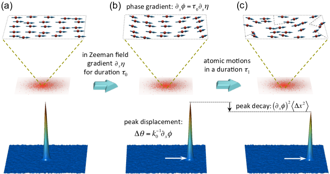
Figure 3: Diffraction images (lower parts) from atomic ensemble in different spin configurations (upper). (a) Spin-coherent-state with in-plane polarization. (b) Evolution in a Zeeman field gradient imprints a phase gradient of spins, resulting in a displacement of the diffraction peak which can be a principle of gradiometer. (c) Atomic motions diminish the spin polarization, resulting in decay of the displaced peak. This can be a principle for non-demolition measurement of atomic temperature and collisional interactions.

Based on this perturbative solution, we analyze the diffraction pattern of Stokes photons as a function of the collection time $\tau_{c}$. We find the weak processes of $\mathcal{L}_{1}$ only result in slow varying modulation of the diffraction pattern, barely changing the ratio of the sharp peak or dip to its neighboring background. Namely,

$$r(\tau_{c})\equiv\frac{n(\theta=0,\tau_{c})-n(\theta_{b},\tau_{c})}{n(\theta_{b},\tau_{c})}\cong\frac{P}{\langle\hat{N}_{s}\rangle-P/N}$$ (8)

where $n(\theta,\varphi,\tau_{c})\equiv\delta\Omega\int_{0}^{\tau_{c}}dtI(\theta,\varphi,t)$ is the number of photons emitted into an infinitesimal solid angle in the collection interval $0\leq t\leq\tau_{c}$. For a dilute ensemble Eq. (8) holds for arbitrarily large $\tau_{c}$ (cf. Fig. 2 (d)). Thus the pair-correlation sum can be faithfully read out from the diffraction pattern of all photons, not limited to those initial ones.

We estimate the range of applicability of our treatment. The dilute condition is satisfied by typical cold atom gases of a density $10^{10}-10^{12}$ cm^-3 or by atoms in optical lattice. The duration of Stokes photon emission is of a timescale $\Gamma^{-1}=(\frac{\Omega_{L}}{2\Delta})^{-2}\Gamma_{0}^{-1}$. The excited state decay rate $\Gamma_{0}\gtrsim 30~{}\mu$s^-1 for typical alkali atoms. quantum_memory0 ; quantum_memory1 ; quantum_memory2 ; quantum_memory3 ; quantum_memory4 ; Pan_quantummemory ; dephaseinOL1 ; dephaseinOL2 Taking $(\frac{\Omega_{L}}{2\Delta})^{-2}\sim 40$, all Stokes photons are emitted in a timescale $\Gamma^{-1}\lesssim~{}\mu$s. For cold atom gases with a temperature of $1-100~{}\mu$K, the average velocity is $0.01-0.1$ m/s. Atoms can only travel $10-100$ nm in the duration of $\Gamma^{-1}$ which is indeed negligible as compared to the light wavelength.

V Field Gradiometer and non-demolition probe of atomic motions and temperature

Under free evolution, the pair-correlation changes as $\textrm{Tr}[\hat{\sigma}_{i^{\prime}}^{+}\hat{\sigma}_{i}^{-}\rho(\tau)]=e^{i(\eta_{i}\tau-\eta_{i^{\prime}}\tau)-2\gamma\tau}\textrm{Tr}[\hat{\sigma}_{i^{\prime}}^{+}\hat{\sigma}_{i}^{-}\rho(0)]$, where $\eta_{i}$ is the Zeeman frequency and $\gamma$ the homogeneous dephasing rate of an individual spin. The pair-correlation sum thus decays only at the single spin dephasing rate. Therefore entanglement in $\rho(0)$ can be reliably detected from the dephased state $\rho(\tau)$ as long as $\tau\ll\gamma^{-1}$, even when the fidelity is exponentially small with $N$ Duan2011 .

Spatial inhomogeneity of external fields leads to position dependent Zeeman frequency $\eta(\mathbf{r})$ and hence inhomogeneous precessions of spins. If the size of the ensemble is small compared to the variation length scale of the field, the dominating term is the gradient: $\eta(\mathbf{r})\cong\mathbf{r}\cdot\mathbf{\nabla}\eta$. For an ensemble initially in a permutation-symmetric state, after an interval $\tau_{0}$ with frozen motion in the Zeeman field gradient, the diffraction pattern becomes $I_{c}=\langle\hat{N}_{s}\rangle-\frac{P}{N-1}+\frac{P}{N^{2}-N}|\langle\sum_{j}e^{-i(\Delta\mathbf{k}-\tau_{0}\mathbf{\nabla}\eta)\cdot\mathbf{r}_{j}}\rangle|^{2}$. We focus on situations where $\partial_{z}\eta$ is either zero or not picked up by atomic ensembles of a quasi-2D geometry in $x-y$ plane. The in-plane gradient simply results in a displacement of the sharp diffraction peak or dip, preserving its strength and shape (Fig. 3). This has several significant consequences. First, by evolution in an external field of known gradient, entanglement can be detected by measuring the peak or dip along a chosen direction with finite $\theta$, such that detectors do not pick up laser photons. Second, the displacement measures the vector value of the gradient. It can thus be used as a principle of vector gradiometer of magnetic field, static electric field via dc Stark effect, and light field via ac Stark effect dephaseinOL1 .

An ideal probe state is the spin-coherent-state of $N$ unentangled atoms with in-plane polarization, which can be realized by optical pumping followed by a spin rotation to the in-plane direction. The gradient is then probed simultaneously by the $\sim N^{2}$ classical pair-correlations, and its vector value is encoded as the displacement of a diffraction peak with strength $\sim N^{2}$.

Now we analyze the sensitivity of our diffraction based Zeeman field gradiometer. Consider the atoms of a 1D geometry illustrated in Fig. 4 (a) with a Gaussian spatial distribution of full-width-half-maximum (FWHM) $A$. Atoms are initialized in the spin-coherent-state and evolved in the Zeeman field gradient for an interval of $\tau_{0}$. The diffraction pattern is then: $\frac{N^{2}}{4}f(\theta)+\frac{N}{4}$, where $f(\theta)\equiv\mathrm{e}^{-\frac{(k_{0}A)^{2}}{4}(\theta-\theta_{0})^{2}}$ is a sharp peak centered in a tilted direction: $\theta_{0}=k_{0}^{-1}\tau_{0}\partial_{x}\eta$. Our goal is to extract this direction from the photon statistics. The field gradient can then be inferred based on the above relation. The spatial resolution of the gradiometer is just given by the size of the atomic ensemble $A$. The precision of this measurement is determined by the width of the peak ($\frac{1}{k_{0}A}$), the shot noise of the photon counts and the angular resolution ($\delta\theta$) of the CCD detector array. While the CCD angular resolution can always be improved by increasing the distance from the atomic ensemble, the former two factors will determine the quantum limit for the sensitivity of this gradiometer. We will examine the increase of the sensitivity with number of atoms $N$ used in the probe. Our discussion is limited to the dilute regime (i.e. $k_{0}A/N\geq 2\pi$).

In a single probe using $N$ atoms, the photon counts at each CCD pixel can be written as $n_{i}+\Delta n_{i}$, where $n_{i}$ and $\Delta n_{i}$ are respectively the expectation value and fluctuation of the photon counts. We have

$$n_{i} = \int_{\theta_{i}-\frac{\delta\theta}{2}}^{\theta_{i}+\frac{\delta\theta}{2}}d\theta\bigg{(}\frac{N^{2}}{4}f(\theta)+\frac{N}{4}\bigg{)}$$

$$= \delta\theta\frac{N^{2}}{4}\bar{f}(\theta_{i})+\delta\theta\frac{N}{4},$$

where $\bar{f}(\theta_{i})\equiv\frac{1}{\delta\theta}\int_{\theta_{i}-\frac{\delta\theta}{2}}^{\theta_{i}+\frac{\delta\theta}{2}}d\theta f(\theta)$. Here we assume that the $i$-th pixel of the detector collects all photons emitted within the angle range $[\theta_{i}-\frac{\delta\theta}{2},\theta_{i}+\frac{\delta\theta}{2}]$, where $\theta_{i}\equiv i\delta\theta$. As shown in Appendix B, the photon statistics is found to be Poissonian when the probe state is spin-coherent-state, and we have

$$\langle\Delta n^{2}_{i}\rangle\sim n_{i},$$ (10)

From the photon statistics $\{n_{i}+\Delta n_{i}\}$, we can extract a peak central position $\theta_{c}$ defined as

$$\theta_{c}=\frac{\sum_{i}\theta_{i}(n_{i}+\Delta n_{i})}{\sum_{i}(n_{i}+\Delta n_{i})}.$$ (11)

$\theta_{c}$ unavoidably has some deviation from $\theta_{0}$, the peak position precision is then defined as $\sqrt{(\theta_{c}-\theta_{0})^{2}}$. Our analysis shows that (see Appendix C), when $\theta_{c}$ from a single probe is used to extract the Zeeman field gradient $\partial_{x}\eta$, the overall precision is

$$\Delta(\partial_{x}\eta)\sim\frac{k_{0}}{\tau_{0}}\sqrt{\frac{4\pi^{-1/2}}{N^{2}k_{0}A}+(k_{0}A)^{4}\delta\theta^{6}}$$ (12)

For small $\delta\theta$, the sensitivity is $\Delta(\partial_{x}\eta)\sim\frac{k_{0}}{\tau_{0}}\frac{1}{N\sqrt{k_{0}A}}$ which scales inversely with $N$.

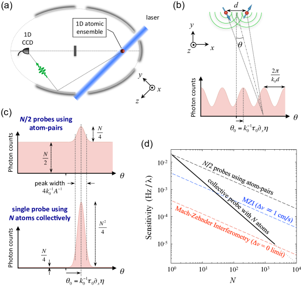
Figure 4: Zeeman field gradiometer using a 1D atomic ensemble. (a) and (b) Schematic of the setup. The ensemble and a 1D CCD array are placed respectively on the two common focus lines of a group of elliptical cylinder mirrors. The mirrors ensure the majority of photons is collected by the detector. The smallest ensemble can be an atom-pair, giving a direct analog of the double-slit interferometry. (c) Signal of $\frac{N}{2}$ probes using atom-pairs (upper), and single probe using $N$ atoms collectively (lower), with each atom placed randomly on the focus line according to a Gaussian distribution with FWHM $A$. The peak strength of the lower is enhanced by a factor of $N$. (d) Gradiometer sensitivity at a spatial resolution $A=1$ mm with a resource of $N$ unentangled atoms. The diffraction based gradiometer using $N$ atoms collectively ($\frac{N}{2}$ atom-pairs independently) has a sensitivity of the $\frac{1}{N}$ ($\frac{1}{\sqrt{N}}$) scaling, shown by the solid (dashed) black line. Sensitivity of flying atom Mach-Zehnder interferometry (MZI) gradiometer is shown for reference. MZI_gradiometer1 The probe time $\tau_{0}=\frac{A}{\Delta v}=0.1$ s for the blue line, limited by a finite velocity uncertainty $\Delta v=1~{}$cm/s, while $\tau_{0}=1$ s for all other lines, limited only by the single spin dephasing time.

The smallest ensemble for the gradiometer can just be an atom pair prepared on spin-coherent-state which emit one photon on average in each probe. We can make $N/2$ independent probes using such atom pairs and extract the field gradient from the integrated signal. For one atom at position $\mathbf{x}_{1}$ and the other atom at $\mathbf{x}_{2}$, the photon has an emission distribution of $\sim 1+\frac{1}{2}\cos\mathbf{k}\cdot(\mathbf{x}_{1}-\mathbf{x}_{2})$ (see Fig. 4 (b)). This is a direct analog of the double-slit interferometry. We assume each atom has fixed position during a single probe but it can randomly appear in a 1D line according to a Gaussian distribution $\propto\mathrm{e}^{-2x^{2}/A^{2}}$ with full-width-half-maximum $A$ for multiple probes. Summing over $N/2$ probes, the total photon distribution pattern is $\frac{N}{2}+\frac{N}{4}\mathrm{e}^{-(k_{x}A)^{2}/4}$. The peak strength is thus $\sim N$. Following the previous derivations, we find sensitivity of measuring the Zeeman field gradient is $\frac{k_{0}}{\tau_{0}}\frac{1}{\sqrt{Nk_{0}A}}$ with the $1/\sqrt{N}$ scaling.

Thus, a single collective probe using $N$ atoms has sensitivity $\sim\frac{1}{N}\frac{k_{0}}{\tau_{0}\sqrt{k_{0}A}}$, which goes beyond the SQL of $\sim\frac{1}{\sqrt{N}}\frac{k_{0}}{\tau_{0}\sqrt{k_{0}A}}$ for $N/2$ independent probes using atom-pairs, as shown in Fig. 4 (d). The enhancement comes from the $N^{2}$ scaling of the peak strength, which is the result of using large group of atoms collectively. In Fig. 4 (d), we also compare with the gradiometer based on Mach-Zehnder interferometer (MZI) of flying atoms in atomic fountain which has the SQL sensitivity of $\sim\frac{1}{\sqrt{N}}\frac{1}{\tau_{0}A}$, while the inevitable velocity uncertainty further sets a tighter upper bound for $\tau_{0}$ dependent on the spatial resolution $A$ (see Appendix D).

The collectively-enhanced sensitivity with $1/N$ scaling is valid in the dilute regime $N\leq k_{0}A$. Beyond this regime, the multiple light scattering can not be treated perturbatively and its effect will eventually renormalize the peak strength to the $N$ scaling. By trapping atoms in optical lattices, the probe time $\tau_{0}$ can be as long as the single spin homogeneous dephasing time, in the order of second or longer dephaseinOL1 . This diffraction based gradiometer using stationary atoms is immune to collective noises and uncertainty in atomic positions, and can have a fine spatial resolution (given by the size of the ensemble). Remarkably, for the scheme to work, the probe state does not need to have high degree of spin polarization as an imperfect polarization $p$ just scales down the sensitivity by $1/p$.

The diffraction image can also be used for non-demolition probe of atomic motions and temperature in trapped cold atom gases, by introducing a waiting time $\tau_{1}$ between the imprinting of phase gradient $\nabla\phi$ on the spin-coherent-state and the measurement of the Stokes photon diffraction (Fig. 3). Atomic motions in the interval $\tau_{1}$ will diminish the spin polarization, resulting in decay of the displaced diffraction peak Pan_quantummemory . For $|\nabla\phi|^{2}\langle\Delta\mathbf{r}^{2}\rangle\ll 1$, the peak strength is $\frac{N^{2}}{4}e^{-|\nabla\phi|^{2}\langle\Delta\mathbf{r}^{2}\rangle/3}$, $\langle\Delta\mathbf{r}^{2}\rangle$ being the mean square displacement of atoms. For short $\tau_{1}$ when $\Delta\mathbf{r}$ is small compared to the interatomic distance $d$, $\langle\Delta\mathbf{r}^{2}\rangle=2\frac{k_{B}T}{m}\tau_{1}^{2}$. Thus, by preparing a large phase gradient $|\nabla\phi|\sim 1/d$, the short time motion can be probed and the atomic temperature can be read out from the decay of the peak. Smaller $|\nabla\phi|$ allows the probe of long time motion which will eventually crossover to the diffusive regime by atom collisions. $\tau_{1}$ is upper limited by the spin dephasing time, which is long enough for observing the entire crossover behavior from ballistic to diffusive motions, providing information about the collisional interactions in trapped gases. The collectively enhanced peak strength of $\sim N^{2}$ provides sufficient signal-to-noise ratio for determining $\langle\Delta\mathbf{r}^{2}\rangle$ at a given $\tau_{1}$ by a single shot measurement.

VI Summary

In conclusion, we have shown that the far field diffraction image of spontaneously emitted Raman photons can be used for detection of spin entanglement in cold atomic ensembles as well as for quantum metrology applications. For many-body states with small or maximum uncertainty in spin-excitation number, entanglement is witnessed by the presence of either a sharp diffraction peak or dip. For general states, the relative strength of the peak or dip over its background detects entanglement through the pair-correlation sum rules derived from spin squeezing inequalities. Spin precessions in Zeeman field gradient lead to displacement of the diffraction peak or dip while atomic motions lead to decay of its strength. These can serve as principles for vector gradiometer of fields and for non-demolition measurement of atomic temperature and collisional dynamics. The gradiometer sensitivity can reach $1/N$ by using a spin-coherent-state of $N$ unentangled atoms as the probe, which suggests a new possibility for going beyond the SQL without entanglement. Motional dynamics leads to temporal decay of the diffraction peak which can be used for non-demolition probe of temperature and collisional interactions in trapped atomic gases.

VII Acknowledgments

The authors thank Lian-ao Wu for helpful discussions. WY thanks CQI at IIIS of Tsinghua for hospitality during his visit through the support by NBRPC under grant 2011CBA00300 (2011CBA00301). The work was supported by the Research Grant Council of Hong Kong under grant HKU706711P and HKU8/CRF/11G.

Appendix A Perturbative Solution to the Master Equation

We assume the wave vector $\mathbf{k}_{0}$ of the driving laser is perpendicular to the ensemble (i.e. $\mathbf{k}_{0}\cdot\mathbf{r}_{i}=0$). For the simplicity of expression, below we replace $\Delta\mathbf{k}\equiv\mathbf{k}-\mathbf{k}_{0}$ by $\mathbf{k}$ when it appears in $\hat{J}^{-}(\Delta\mathbf{k})$.

The collected photon number in a time $\tau_{c}$ along direction $\mathbf{k}$ within the infinitesimal solid angle $\delta\Omega$ writes $n_{p}(\mathbf{k},\tau_{c})=\Gamma\frac{\delta\Omega}{4\pi}\int_{0}^{\tau_{c}}dt\textrm{Tr}[\hat{J}^{+}(\mathbf{k})\hat{J}^{-}(\mathbf{k})\rho(t)]$. Here we have ignored the slowly varying single atom dipole emission pattern. $\rho(t)$ can be solved from the master equation (Eq. (7)) by viewing the $\mathcal{L}_{1}$ term as perturbation.

We use the notation $\rho^{(n)}(t)$ and $\langle\cdots\rangle^{(n)}_{t}\equiv\textrm{Tr}[\cdots\rho^{(n)}(t)]$ to describe the result keeping up to $n$-th order effect of $\mathcal{L}_{1}$. For the $0$-th order result $\rho^{(0)}(t)=\mathrm{e}^{\mathcal{L}_{0}t}\rho(0)$, there is $\langle\hat{\sigma}_{m}^{+}\hat{\sigma}_{n}^{-}\rangle^{(0)}_{t}=\mathrm{e}^{-\Gamma t}\langle\hat{\sigma}_{m}^{+}\hat{\sigma}_{n}^{-}\rangle_{0}$. Then

$$n_{p}^{(0)}(\mathbf{k},\tau_{c})=\frac{\delta\Omega}{4\pi}(1-\mathrm{e}^{-\Gamma\tau_{c}})\langle\hat{J}^{+}(\mathbf{k})\hat{J}^{-}(\mathbf{k})\rangle_{0}.$$ (13)

Below we solve for $\rho^{(1)}(t)$ which captures the leading order effect of $\mathcal{L}_{1}$, and show that it is sufficient to account for the effect of $\mathcal{L}_{1}$ under the dilute limit. We consider an $N$-atom 1D lattice. In the 1-st order approximation, the equation of motion for the pair-correlation is

$$\frac{d\langle\hat{\sigma}_{m}^{+}\hat{\sigma}_{n}^{-}\rangle^{(1)}_{t}}{d(\Gamma t)}= -\langle\hat{\sigma}_{m}^{+}\hat{\sigma}_{n}^{-}\rangle^{(1)}_{t}$$

$$+\sum_{j\neq n}(\frac{\Gamma_{jn}}{2\Gamma}-i\frac{G_{jn}}{2\Gamma})\langle\hat{\sigma}_{m}^{+}\hat{\sigma}_{j}^{-}\hat{\sigma}_{n}^{z}\rangle^{(0)}_{t}$$

$$+\sum_{j\neq m}(\frac{\Gamma_{jm}}{2\Gamma}+i\frac{G_{jm}}{2\Gamma})\langle\hat{\sigma}_{m}^{z}\hat{\sigma}_{j}^{+}\hat{\sigma}_{n}^{-}\rangle^{(0)}_{t}.$$ (14)

We denote $\Gamma_{j}\equiv\Gamma_{n\pm j,n}=\Gamma\frac{\sin|jkd|}{|jkd|}$, $G_{j}\equiv G_{n\pm j,n}=\Gamma\frac{\cos|jkd|}{|jkd|}$, and $a^{(0)}_{t}\equiv\langle\hat{\sigma}_{m}^{+}\hat{\sigma}_{m}^{-}\rangle^{(0)}_{t}$ , $p^{(0)}_{t}\equiv\langle\hat{\sigma}_{m}^{+}\hat{\sigma}_{n}^{-}\rangle^{(0)}_{t,m\neq n}$. Then

$$\frac{d\langle\hat{\sigma}_{n}^{+}\hat{\sigma}_{n}^{-}\rangle^{(1)}_{t}}{d(\Gamma t)}= -\langle\hat{\sigma}_{n}^{+}\hat{\sigma}_{n}^{-}\rangle^{(1)}_{t}-p^{(0)}_{t}\Big{(}\sum_{j=1}^{N-n}+\sum_{j=1}^{n-1}\Big{)}\frac{\Gamma_{j}}{\Gamma},$$

$$\frac{d\langle\hat{\sigma}_{m}^{+}\hat{\sigma}_{n}^{-}\rangle^{(1)}_{t,m\neq n}}{d(\Gamma t)}= -\langle\hat{\sigma}_{m}^{+}\hat{\sigma}_{n}^{-}\rangle^{(1)}_{t,m\neq n}+2B^{(0)}_{t}\frac{\Gamma_{m-n}}{\Gamma}$$

$$+\alpha^{(0)}_{t}\Big{(}\sum_{j=1}^{N-n}+\sum_{j=1}^{n-1}\Big{)}\big{(}\frac{\Gamma_{j}}{\Gamma}-i\frac{G_{j}}{\Gamma}\big{)}$$

$$+\alpha^{(0)}_{t}\Big{(}\sum_{j=1}^{N-m}+\sum_{j=1}^{m-1}\Big{)}\big{(}\frac{\Gamma_{j}}{\Gamma}+i\frac{G_{j}}{\Gamma}\big{)}.$$ (15)

Where $\alpha^{(0)}_{t}\equiv\frac{1}{2}\langle\hat{\sigma}_{j}^{+}\hat{\sigma}_{m}^{-}\hat{\sigma}_{n}^{z}\rangle^{(0)}_{t,j\neq m\neq n}$ is the three-body correlation, $B^{(0)}_{t}\equiv\frac{1}{2}\langle\hat{\sigma}_{m}^{+}\hat{\sigma}_{m}^{-}\hat{\sigma}_{n}^{z}\rangle^{(0)}_{t,m\neq n}-\alpha^{(0)}_{t}$.

Using $\langle\hat{J}^{+}(\mathbf{k})\hat{J}^{-}(\mathbf{k})\rangle^{(1)}_{t}=\sum_{n}\langle\hat{\sigma}_{n}^{+}\hat{\sigma}_{n}^{-}\rangle^{(1)}_{t}+\sum_{m\neq n}\mathrm{e}^{i\mathbf{k}\cdot(\mathbf{r}_{m}-\mathbf{r}_{n})}\langle\hat{\sigma}_{m}^{+}\hat{\sigma}_{n}^{-}\rangle^{(1)}_{t}$, and switching the summation index as

$$\sum_{n=1}^{N}\Big{(}\sum_{j=1}^{N-n}+\sum_{j=1}^{n-1}\Big{)}=\sum_{j=1}^{N-1}\Big{(}\sum_{n=1}^{N-j}+\sum_{n=j+1}^{N}\Big{)},$$ (16)

we write

$$\frac{d\langle\hat{J}^{+}(\mathbf{k})\hat{J}^{-}(\mathbf{k})\rangle^{(1)}_{t}}{d(\Gamma t)}$$

$$= -\langle\hat{J}^{+}(\mathbf{k})\hat{J}^{-}(\mathbf{k})\rangle^{(1)}_{t}$$

$$+4(N-j)\sum_{j=1}^{N-1}\frac{\Gamma_{j}}{\Gamma}\big{(}B^{(0)}_{t}\cos(j\mathbf{k}\cdot\mathbf{d})-\frac{1}{2}p^{(0)}_{t}-\alpha^{(0)}_{t}\big{)}$$

$$+\alpha^{(0)}_{t}\Big{[}\sum_{j=1}^{N-1}\big{(}\frac{\Gamma_{j}}{\Gamma}-i\frac{G_{j}}{\Gamma}\big{)}f_{j}(\mathbf{k})+\textrm{C.c.}\Big{]}.$$ (17)

Where $\mathbf{d}$ is the vector connecting neighboring atoms, and

$$f_{j}(\mathbf{k})\equiv \bigg{(}\sum_{m=1}^{N}\mathrm{e}^{i\mathbf{k}\cdot\mathbf{r}_{m}}\bigg{)}\bigg{(}\sum_{n=1}^{N-j}+\sum_{n=j+1}^{N}\bigg{)}\mathrm{e}^{-i\mathbf{k}\cdot\mathbf{r}_{n}}$$

$$= 2\cos^{2}\frac{j\mathbf{k}\cdot\mathbf{d}}{2}\frac{\sin^{2}\frac{N\mathbf{k}\cdot\mathbf{d}}{2}}{\sin^{2}\frac{\mathbf{k}\cdot\mathbf{d}}{2}}-\frac{\sin(N\mathbf{k}\cdot\mathbf{d})\sin(j\mathbf{k}\cdot\mathbf{d})}{2\sin^{2}\frac{\mathbf{k}\cdot\mathbf{d}}{2}}.$$ (18)

As $\Gamma_{j},G_{j}\sim\frac{1}{jkd}$, only those $j$ terms with $j\ll N$ make significant contributions. Thus $\frac{\sin(N\mathbf{k}\cdot\mathbf{d})\sin(j\mathbf{k}\cdot\mathbf{d})}{2\sin^{2}\frac{\mathbf{k}\cdot\mathbf{d}}{2}}$ can be ignored compared to $\cos^{2}\frac{j\mathbf{k}\cdot\mathbf{d}}{2}\frac{\sin^{2}\frac{N\mathbf{k}\cdot\mathbf{d}}{2}}{\sin^{2}\frac{\mathbf{k}\cdot\mathbf{d}}{2}}$. Then

$$\frac{d\langle\hat{J}^{+}(\mathbf{k})\hat{J}^{-}(\mathbf{k})\rangle^{(1)}_{t}}{d(\Gamma t)}$$

$$\approx -\langle\hat{J}^{+}(\mathbf{k})\hat{J}^{-}(\mathbf{k})\rangle^{(1)}_{t}$$

$$+\frac{2\alpha^{(0)}_{t}}{p^{(0)}_{t}}\sum_{j>0}\frac{\Gamma_{j}}{\Gamma}\big{(}\cos(j\mathbf{k}\cdot\mathbf{d})+1\big{)}\langle\hat{J}^{+}(\mathbf{k})\hat{J}^{-}(\mathbf{k})\rangle^{(0)}_{t}$$

$$+N\sum_{j>0}\frac{\Gamma_{j}}{\Gamma}\Big{(}C_{2}\cos(j\mathbf{k}\cdot\mathbf{d})+C_{3}\Big{)},$$ (19)

with $C_{2}\equiv 4B^{(0)}_{t}-2\alpha^{(0)}_{t}(\frac{a^{(0)}_{t}}{p^{(0)}_{t}}-1)$ and $C_{3}\equiv-2p^{(0)}_{t}-2\alpha^{(0)}_{t}(\frac{a^{(0)}_{t}}{p^{(0)}_{t}}+1)$. In the above equation we have used the relation $\langle\hat{J}^{+}(\mathbf{k})\hat{J}^{-}(\mathbf{k})\rangle^{(0)}_{t}=N(a^{(0)}_{t}-p^{(0)}_{t})+p^{(0)}_{t}\frac{\sin^{2}\frac{N\mathbf{k}\cdot\mathbf{d}}{2}}{\sin^{2}\frac{\mathbf{k}\cdot\mathbf{d}}{2}}$.

The time dependence of $a^{(0)}_{t}$, $p^{(0)}_{t}$, $\alpha^{(0)}_{t}$ and $B^{(0)}_{t}$ are easily obtained from $\rho^{(0)}(t)$:

$$a^{(0)}_{t}= ~{}\mathrm{e}^{-\Gamma t}a^{(0)}_{0},~{}~{}~{}~{}~{}~{}p^{(0)}_{t}=\mathrm{e}^{-\Gamma t}p^{(0)}_{0},$$

$$\alpha^{(0)}_{t}= ~{}\mathrm{e}^{-2\Gamma t}\alpha^{(0)}_{0}-\frac{1}{2}\mathrm{e}^{-\Gamma t}(1-\mathrm{e}^{-\Gamma t})p^{(0)}_{0},$$

$$B^{(0)}_{t}= ~{}\frac{1}{4}\mathrm{e}^{-2\Gamma t}\big{\langle}(\hat{\sigma}_{m}^{z}+1)(\hat{\sigma}_{n}^{z}+1)\big{\rangle}_{0}$$

$$~{}-\frac{1}{2}\mathrm{e}^{-\Gamma t}a^{(0)}_{0}-\alpha^{(0)}_{t}.$$ (20)

Solving the differential equation Eq. (19), we obtain the photon diffraction pattern under the $1$-st order approximation:

$$n_{p}^{(1)}(\mathbf{k},\tau_{c})=\Gamma\frac{\delta\Omega}{4\pi}\int_{0}^{\tau_{c}}dt\langle\hat{J}^{+}(\mathbf{k})\hat{J}^{-}(\mathbf{k})\rangle_{t}$$

$$\approx ~{}\frac{\delta\Omega}{4\pi}N\sum_{j>0}\frac{\Gamma_{j}}{\Gamma}\bigg{[}f_{2}(\tau_{c})\cos(j\mathbf{k}\cdot\mathbf{d})+f_{3}(\tau_{c})\bigg{]}$$

$$~{}+\frac{\delta\Omega}{4\pi}\bigg{[}1-\mathrm{e}^{-\Gamma\tau_{c}}+f_{1}(\tau_{c})\sum_{j>0}\frac{\Gamma_{j}}{\Gamma}\big{(}\cos(j\mathbf{k}\cdot\mathbf{d})+1\big{)}\bigg{]}$$

$$~{}~{}~{}~{}~{}~{}\times\langle\hat{J}^{+}(\mathbf{k})\hat{J}^{-}(\mathbf{k})\rangle_{0},$$ (21)

where

$$f_{1}(\tau_{c})= ~{}(1-\mathrm{e}^{-\Gamma\tau_{c}})^{2}\frac{\alpha^{(0)}_{0}}{p^{(0)}_{0}}+\tau_{c}\mathrm{e}^{-\Gamma\tau_{c}}+\frac{1}{2}\mathrm{e}^{-2\Gamma\tau_{c}}-\frac{1}{2},$$

$$f_{2}(\tau_{c})= ~{}\frac{1}{2}(1-\mathrm{e}^{-\Gamma\tau_{c}})^{2}\big{\langle}(\hat{\sigma}_{m}^{z}+1)(\hat{\sigma}_{n}^{z}+1)\big{\rangle}_{0}$$

$$+(1-\Gamma\tau_{c}\mathrm{e}^{-\Gamma\tau_{c}}-\mathrm{e}^{-\Gamma\tau_{c}})(p^{(0)}_{0}-a^{(0)}_{0})$$

$$-(1-\mathrm{e}^{-\Gamma\tau_{c}})^{2}\Big{(}\frac{\alpha^{(0)}_{0}}{p^{(0)}_{0}}+\frac{1}{2}\Big{)}\big{(}a^{(0)}_{0}+p^{(0)}_{0}\big{)},$$

$$f_{3}(\tau_{c})= -(1-\mathrm{e}^{-\Gamma\tau_{c}})^{2}\Big{(}\frac{\alpha^{(0)}_{0}}{p^{(0)}_{0}}+\frac{1}{2}\Big{)}\big{(}a^{(0)}_{0}+p^{(0)}_{0}\big{)}$$

$$+(1-\Gamma\tau_{c}\mathrm{e}^{-\Gamma\tau_{c}}-\mathrm{e}^{-\Gamma\tau_{c}})\big{(}a^{(0)}_{0}-p^{(0)}_{0}\big{)}.$$ (22)

$f_{1}(\tau_{c}),f_{2}(\tau_{c}),f_{3}(\tau_{c})\sim O\big{(}(\Gamma\tau_{c})^{2}\big{)}$ for $\Gamma\tau_{c}\ll 1$.

Comparing Eq. (13) and Eq. (21), we can see that the modulation of the diffraction pattern by the multiple-light scattering is described by $\cos(j\mathbf{k}\cdot\mathbf{d})$. The dipole-dipole interaction with coefficients $G_{j}$ has a vanishing $1$-st order effect, thus it does not appear in our above derivation. Obviously for $j\ll N$ the modulation is slowly varying in $\mathbf{k}$ space. We are interested only in the diffraction pattern in the neighborhood of the forward direction where $\cos(j\mathbf{k}\cdot\mathbf{d})\approx 1$, then $n_{p}^{(1)}(\tau_{c}\to\infty)=\beta_{1}n_{p}^{(0)}(\tau_{c}\to\infty)+\frac{\delta\Omega}{4\pi}N\beta_{2}$, with $\beta_{1}=1+2f_{1}(\tau_{c}\to\infty)\sum_{j>0}\frac{\Gamma_{j}}{\Gamma}$ and $\beta_{2}=[f_{2}(\tau_{c}\to\infty)+f_{3}(\tau_{c}\to\infty)]\sum_{j>0}\frac{\Gamma_{j}}{\Gamma}$. The peak/dip to background ratio of the initial diffraction pattern (i.e. $\tau_{c}\to 0$) is $r^{(0)}=\frac{N^{2}p^{(0)}_{0}}{N[a^{(0)}_{0}-p^{(0)}_{0}]}$ which measures the pair-correlation sum of the initial atomic state of interest. In the diffraction pattern of all emitted photons (i.e. $\tau_{c}\to\infty$), it becomes

$$r^{(1)} = \frac{\beta_{1}N^{2}p^{(0)}_{0}+N\beta_{2}}{\beta_{1}N[a^{(0)}_{0}-p^{(0)}_{0}]+N\beta_{2}}=(1+\delta)r^{(0)},$$

$$\delta \cong \frac{\beta_{2}}{\beta_{1}[a^{(0)}_{0}-p^{(0)}_{0}]+\beta_{2}}.$$ (23)

Since $\sum_{j>0}\frac{\Gamma_{j}}{\Gamma}\approx\frac{1}{kd}\int_{0}^{\infty}\frac{\sin x}{x}dx\sim\frac{1}{kd}\ll 1$, we expect $\beta_{1}\approx 1$ and $\beta_{2}\ll 1$. Thus $\delta\ll 1$. When the initial atomic state is an eigenstate of $\hat{J}_{z}$ or a separable state, we have

$$\delta\cong\frac{-2a^{(0)}_{0}p^{(0)}_{0}\sum_{j>0}\frac{\Gamma_{j}}{\Gamma}}{a^{(0)}_{0}-p^{(0)}_{0}}.$$ (24)

We note that $p^{(0)}_{0}=P/(N^{2}-N)$, which has the maximum value of $1/4$ in the neighborhood of Dicke state with half-spin-excitation. For typical states, $p^{(0)}_{0}\sim 1/N$ and then $\delta$ scales inversely with $N$.

To examine the convergence of the perturbation solution, we compare it with exact numerical solution of the master equation for a small ensemble in an 1D lattice with various lattice constant $d$. The magnitude of the multiple-light scattering terms in $\mathcal{L}_{1}$ decays fast with the distance, thus only the nearest neighbor terms are important. Because of the limit of computation capability, in the calculation presented in Fig. 5, 6 and 7 when referring to multiple-light scattering, we only keep the nearest neighbor terms in $\mathcal{L}_{1}$ (i.e. those with coefficients $\Gamma_{1}$) and artificially set $\Gamma_{j}=0$ for $j\geq 2$. But for dipole-dipole interaction all $G_{j}$ terms are considered in the exact numerical solution. For this reduced master equation, we compare the perturbative solution and exact numerical solution. We can see the perturbative solution keeping the 1st order effect of $\mathcal{L}_{1}$ (i.e. Eq. (21)) has excellent convergence to the exact numerical solution for both the dip pattern and peak pattern. In particular, the multiple light scattering has negligible effects if we set the collection time $T\leq 0.1/\Gamma$. Note that in the initial interval of $T=0.1/\Gamma$, $10\%$ of all spin-excitations are already converted into Stokes photons. In Fig. 8, we show that effects of next-nearest neighbor terms in $\mathcal{L}_{1}$ (i.e. with coefficients $\Gamma_{2}$ and $\Gamma_{3}$) are also well accounted by the perturbative solutions in Eq. (21). This calculation also confirms that the modulation of the diffraction pattern is dominated by the near neighbor cross terms, and the effect of $\Gamma_{3}$ term is already small as compared to the $\Gamma_{1}$ and $\Gamma_{2}$ terms.

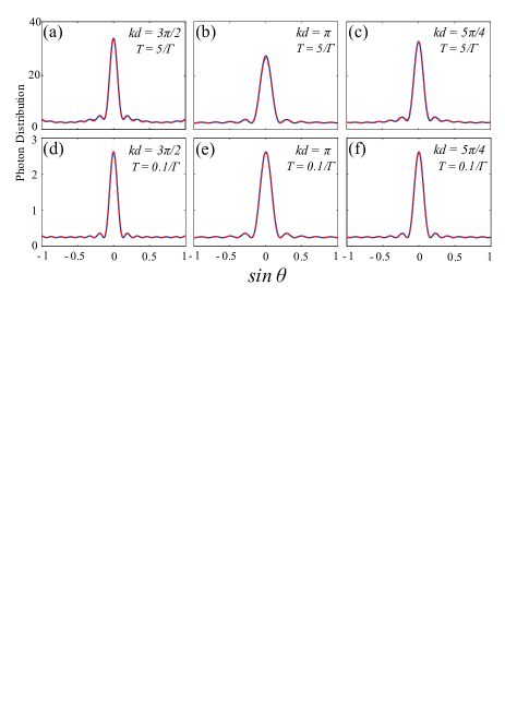
Figure 5: Diffraction pattern of Stokes photons emitted by a chain of $10$ atoms initially in the spin-coherent-state with in-plane polarization $\otimes_{j=1}^{10}\frac{|\uparrow\rangle_{j}+|\downarrow\rangle_{j}}{\sqrt{2}}$. With the collection interval $T=5/\Gamma$, $99.3\%$ of all spin-excitations are converted into Stokes photons, and with $T=0.1/\Gamma$, $10\%$ of all spin-excitations are converted into Stokes photons. Red dashed lines: exact numerical solution of the master equation Eq. (7). Blue solid lines in (a-c): perturbative solution keeping the 1st order effect of $\mathcal{L}_{1}$ (i.e. Eq. (21)). Blue solid lines in (d-f): the $0$-th order solution without $\mathcal{L}_{1}$ (i.e. Eq. (13)).

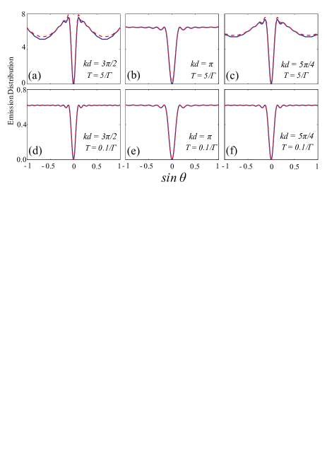
Figure 6: Diffraction pattern of Stokes photons emitted by a chain of $12$ atoms initially in the many-body singlet (i.e. $J=0$, $M=0$). Red dashed lines: exact numerical solution of the master equation Eq. (7). Blue solid lines in (a-c): perturbative solution keeping the 1st order effect of $\mathcal{L}_{1}$ (i.e. Eq. (21)). Blue solid lines in (d-f): the $0$-th order solution without $\mathcal{L}_{1}$ (i.e. Eq. (13)).

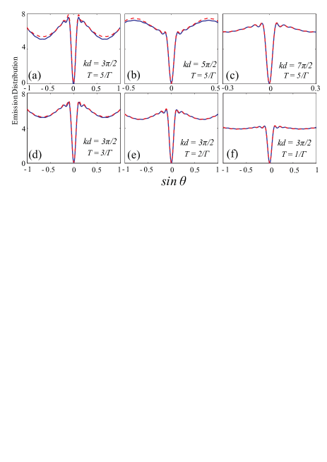
Figure 7: Diffraction pattern of Stokes photons emitted by a chain of $12$ atoms initially in the many-body singlet (i.e. $J=0$, $M=0$) with various duration of the collection time $T$. Red dashed lines: exact numerical solution of the master equation Eq. (7). Blue solid lines: perturbative solution keeping the 1st order effect of $\mathcal{L}_{1}$ (i.e. Eq. (21)).

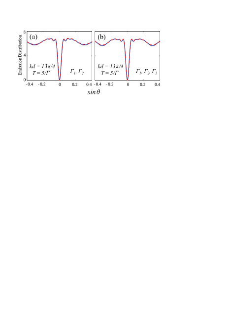
Figure 8: The results which not only includes the nearest neighbor $\Gamma_{1}$ term, but also contains (a) next-nearest neighbor $\Gamma_{2}$ and (b) $\Gamma_{2}$, $\Gamma_{3}$ terms for $12$-qubit $J=0$, $M=0$ permutation invariant state. Values of $d$ and $T$ are given in the figure. Red dashed lines: the numerical simulated results. Blue solid lines: the fitting using Eq. (21). The dipole-dipole interaction $G_{j}$ is not consider here.

We have also considered a 2D atomic ensemble in the $xy$ plane in a large trap, where the atomic number density is Gaussian $n(\mathbf{r})=n(0)\mathrm{e}^{-2r^{2}/A^{2}}$ at position $\mathbf{r}$ with $A$ the full-width-half-maximum (FWHM). The total atom number is given by $N=\int d\mathbf{r}n(\mathbf{r})=\frac{\pi}{2}n(0)A^{2}$ with the dilute condition $k_{0}A\sqrt{N}\geq 2\pi$ satisfied. The result is similar to the case of 1D lattice that the peak/dip to background ratio is only slightly changed.

For dilute hot atomic vapor where atomic motion is much faster than the Stokes photon emission, we find that the diffraction pattern is similar to that of cold atoms in the neighborhood of the forward direction, i.e. with a sharp diffraction peak/dip from which the pair-correlation sum of atoms can be read out. Since atoms move around in a timescale faster than the photon emission, the coefficients of cross terms in $\mathcal{L}_{1}$ should be replaced by $\Gamma_{jj^{\prime}}=\Gamma\big{\langle}\frac{\sin(k_{0}|\mathbf{r}_{j}-\mathbf{r}_{j^{\prime}}|)}{k_{0}|\mathbf{r}_{j}-\mathbf{r}_{j^{\prime}}|}\big{\rangle}_{\textrm{mot}}=\frac{\Gamma}{2(k_{0}A)^{2}}$, $G_{jj^{\prime}}=\frac{G}{(k_{0}A)^{2}}$ which are independent of $j$ and $j^{\prime}$ Wstate . Here $A$ is the size of atomic vapor. The original master equation Eq. (7) becomes

$$\dot{\rho}= ~{}\frac{\Gamma}{2}\sum_{j}\left(2\hat{\sigma}_{j}^{-}\rho\hat{\sigma}_{j}^{+}-\hat{\sigma}_{j}^{+}\hat{\sigma}_{j}^{-}\rho-\rho\hat{\sigma}_{j}^{+}\hat{\sigma}_{j}^{-}\right)$$

$$+\frac{\Gamma}{4(k_{0}A)^{2}}\left(2\hat{J}^{-}\rho\hat{J}^{+}-\hat{J}^{+}\hat{J}^{-}\rho-\rho\hat{J}^{+}\hat{J}^{-}\right)$$

$$+i\frac{G}{2(k_{0}A)^{2}}[\hat{J}_{x}^{2}+\hat{J}_{y}^{2},\rho].$$ (25)

In the RHS of above master equation, the first term corresponds to atoms independently emit photons, the second term comes from multiple light scattering, and the third term is the dipole-dipole interaction. Then

$$\frac{d\langle\hat{J}_{z}\rangle_{t}}{dt}=-\Gamma\left(\frac{N}{2}+\langle\hat{J}_{z}\rangle_{t}\right)-\frac{\Gamma}{2(k_{0}A)^{2}}\langle\hat{J}^{+}\hat{J}^{-}\rangle_{t},$$

$$\frac{d\langle\hat{J}^{+}\hat{J}^{-}\rangle_{t}}{dt}=-\Gamma\langle\hat{J}^{+}\hat{J}^{-}\rangle_{t}+\frac{\Gamma}{(k_{0}A)^{2}}\langle\hat{J}^{+}\hat{J}_{z}\hat{J}^{-}\rangle_{t}.$$ (26)

The angular distribution of the emission rate is given by

$$\langle\hat{J}^{+}(\mathbf{k})\hat{J}^{-}(\mathbf{k})\rangle_{t}$$

$$= ~{}\frac{N}{2}+\langle\hat{J}_{z}\rangle_{t}+\big{(}\langle\hat{J}^{+}\hat{J}^{-}\rangle_{t}-\langle\hat{J}_{z}\rangle_{t}-\frac{N}{2}\big{)}\big{|}\langle\mathrm{e}^{i\Delta\mathbf{k}\cdot\mathbf{r}_{j}}\rangle_{\textrm{mot}}\big{|}^{2}.$$ (27)

Just like the case of dilute cold atom ensemble, the initial diffraction pattern has a sharp diffraction peak/dip in the forward direction with a width given by $\frac{1}{k_{0}A}$, and a strength determined by the pair-correlation sum $P=\langle\hat{J}^{+}\hat{J}^{-}\rangle_{0}-\langle\hat{J}_{z}\rangle_{0}-\frac{N}{2}$. The value of the pair-correlation sum can be read out from the relative ratio of the peak/dip to the neighboring background. From Eq. (26), we can see the background part $\frac{N}{2}+\langle\hat{J}_{z}\rangle_{t}$ in the emission rate decays with time, and the existence of $\frac{\Gamma}{2(k_{0}A)^{2}}\langle\hat{J}^{+}\hat{J}^{-}\rangle_{t}$ term makes the decay faster. On the other hand, the peak/dip strength $\langle\hat{J}^{+}\hat{J}^{-}\rangle_{t}-\langle\hat{J}_{z}\rangle_{t}-\frac{N}{2}$ may increase with time as long as $\frac{\langle\hat{J}^{+}\hat{J}_{z}\hat{J}^{-}\rangle_{t}}{(k_{0}A)^{2}}+\frac{\langle\hat{J}^{+}\hat{J}^{-}\rangle_{t}}{2(k_{0}A)^{2}}>\langle\hat{J}^{+}\hat{J}^{-}\rangle_{t}-\langle\hat{J}_{z}\rangle_{t}-\frac{N}{2}$. This is just the case discussed in the study of superradiance phenomena by Rehler and Eberly Eberly_superradiance , where the authors show that in a very dense ensemble a directional superradiance may develop at later time even when the initial state emission pattern is almost isotropic in all direction and has no superradiance behavior.

Here we are interested in how the peak/dip to background ratio evolves as a function of collection interval. It is obvious that only the second terms in the RHS of both equations in Eq. (26) can change this ratio. When the dilute condition $(k_{0}A)^{2}/N\geq(2\pi)^{2}$ is satisfied, $\frac{\langle\hat{J}^{+}\hat{J}^{-}\rangle_{t}}{2(k_{0}A)^{2}}\ll\frac{N}{2}+\langle\hat{J}_{z}\rangle_{t}$ and $\frac{\langle\hat{J}^{+}\hat{J}_{z}\hat{J}^{-}\rangle_{t}}{(k_{0}A)^{2}}\ll\langle\hat{J}^{+}\hat{J}^{-}\rangle_{t}$, the effects is negligible as compared to the first terms. Thus, the peak/dip to background ratio is barely changed by the multiple light scattering and dipole-dipole interaction when the dilute condition is satisfied.

Appendix B Photon number fluctuations

We analyze the shot noise of the photon counts at the detectors. The total number of Stokes photons in a given direction $\mathbf{k}$ at collection time $\tau_{c}$ is given by $n_{p}(\tau_{c})=\sum_{\mathbf{k}}\langle\hat{a}^{\dagger}_{\mathbf{k}}(\tau_{c})\hat{a}_{\mathbf{k}}(\tau_{c})\rangle$, here the summation is over a finite solid angle $\delta\Omega$. From the effective light-atom coupling Hamiltonian (Eq. (1)), the evolution of the photon operator writes

$$\hat{a}_{\mathbf{k}}(t)=\hat{a}_{\mathbf{k}}(0)\mathrm{e}^{-i\omega_{k}t}\!+ig_{\mathbf{k}}\!\!\int_{0}^{t}\!\!d\tau\hat{J}^{-}(\mathbf{k},\tau)\mathrm{e}^{-i\omega_{\mathbf{k}}(t-\tau)}.$$ (28)

The photon number fluctuation can then be expressed in terms of the atomic correlations

$$\Delta n_{p}^{2} \equiv \Big{\langle}\Big{(}\sum_{\mathbf{k}}\hat{a}^{\dagger}_{\mathbf{k}}(\tau_{c})\hat{a}_{\mathbf{k}}(\tau_{c})\Big{)}^{2}\Big{\rangle}-\Big{\langle}\sum_{\mathbf{k}}\hat{a}^{\dagger}_{\mathbf{k}}(\tau_{c})\hat{a}_{\mathbf{k}}(\tau_{c})\Big{\rangle}^{2}$$ (29)

$$= n_{p}-n_{p}^{2}+\sum_{\mathbf{k}\mathbf{k}^{\prime}}\big{\langle}\hat{a}^{\dagger}_{\mathbf{k}}(\tau_{c})\hat{a}^{\dagger}_{\mathbf{k}^{\prime}}(\tau_{c})\hat{a}_{\mathbf{k}}(\tau_{c})\hat{a}_{\mathbf{k}^{\prime}}(\tau_{c})\big{\rangle}$$

$$= n_{p}-n_{p}^{2}+\frac{2}{(4\pi)^{2}}\int\!d\Omega_{\mathbf{k}}d\Omega_{\mathbf{k}^{\prime}}\int_{0}^{\tau_{c}}\!\!dt_{1}\!\int_{0}^{t_{1}}\!\!\!dt_{2}$$

$$\big{\langle}\hat{J}^{+}(\mathbf{k}^{\prime},t_{2})\hat{J}^{+}(\mathbf{k},t_{1})\hat{J}^{-}(\mathbf{k},t_{1})\hat{J}^{-}(\mathbf{k}^{\prime},t_{2})\big{\rangle}.$$

Here for simplicity we have ignored the slowly varying single atom dipole emission pattern.

In Appendix A, we have shown that the $\mathcal{L}_{1}$ term in the master equation only results in a small modulation on the diffraction pattern. Thus, in deriving $\Delta n_{p}^{2}$ the effect of $\mathcal{L}_{1}$ term will not be considered since we are only interested in the order of magnitude of the fluctuation. From the quantum regression theorem Carmichael_book , we have $\langle\hat{J}^{+}(\mathbf{k}^{\prime},t)\hat{J}^{+}(\mathbf{k},t+\tau)\hat{J}^{-}(\mathbf{k},t+\tau)\hat{J}^{-}(\mathbf{k}^{\prime},t)\rangle=\mathrm{e}^{-\Gamma\tau-2\Gamma t}\textrm{Tr}[\hat{J}^{+}(\mathbf{k}^{\prime})\hat{J}^{+}(\mathbf{k})\hat{J}^{-}(\mathbf{k})\hat{J}^{-}(\mathbf{k}^{\prime})\rho(0)]$. Assuming that a CCD pixel collects photons emitted in a small solid angle $\delta\Omega\lesssim\frac{1}{N}$. During the time interval of $0$ to $\infty$, we find the expectation value and fluctuation in the number of photons collected by a pixel placed in the direction of $\mathbf{k}$:

$$n_{p} \approx \frac{\delta\Omega}{4\pi}\textrm{Tr}\big{[}\hat{J}^{+}(\mathbf{k})\hat{J}^{-}(\mathbf{k})\rho(0)\big{]},$$

$$\Delta n_{p}^{2} \approx \frac{\delta\Omega^{2}}{(4\pi)^{2}}\textrm{Tr}\big{[}\hat{J}^{+}(\mathbf{k})\hat{J}^{+}(\mathbf{k})\hat{J}^{-}(\mathbf{k})\hat{J}^{-}(\mathbf{k})\rho(0)\big{]}$$ (30)

$$+n_{p}-n_{p}^{2}.$$

For atomic ensemble initially in eigenstates of $\hat{J}_{z}$ or spin-coherent-states with in-plane polarization, a straightforward calculation shows $n_{p}\sim N^{2}\delta\Omega\sim N$, $\Delta n_{p}^{2}\sim n_{p}$ for $\mathbf{k}$ in the neighborhood of the forward direction, and $n_{p}\sim N\delta\Omega\sim 1$, $\Delta n_{p}^{2}\sim n_{p}$ for $\mathbf{k}$ away from the forward direction, i. e., the photon statistics is Poissonian.

Appendix C Extraction of the peak position from the photon statistics

The most intuitive way to define the central position from the photon distribution $\{n_{i}+\Delta n_{i}\}$ collected at the CCD pixels is,

$$\theta_{c}=\frac{\sum_{i}\theta_{i}(n_{i}+\Delta n_{i})}{\sum_{i}(n_{i}+\Delta n_{i})}=\bar{\theta}_{c}+\frac{\sum_{i}(\theta_{i}-\bar{\theta}_{c})\Delta n_{i}}{\sum_{i}(n_{i}+\Delta n_{i})}.$$ (31)

Where $\theta_{c}$ is the peak central position extracted from a single probe, and $\bar{\theta}_{c}\equiv\frac{\sum_{i}\theta_{i}n_{i}}{\sum_{i}n_{i}}$ is the expectation value of $\theta_{c}$ in an ensemble measurement consists of many probes. We first show that $\bar{\theta}_{c}$ can infinitely approach $\theta_{0}$ with sufficient resolution of the CCD.

For large $N$, we can neglect the homogeneous background which is by a factor of $N$ smaller than the peak feature, and write

$$\bar{\theta}_{c}=\frac{\sum_{i}\theta_{i}\bar{f}(\theta_{i})}{\sum_{i}\bar{f}(\theta_{i})}=\frac{\int_{\theta_{\textrm{min}}}^{\theta_{\textrm{max}}}d\theta\theta f(\theta)}{\int_{\theta_{\textrm{min}}}^{\theta_{\textrm{max}}}d\theta f(\theta)}+\epsilon=\theta_{0}+\epsilon.$$ (32)

The deviation $\epsilon$ comes from transforming the summation into integral, which writes

$$\epsilon= ~{}\frac{\sum_{i}\int_{\theta_{i}-\frac{\delta\theta}{2}}^{\theta_{i}+\frac{\delta\theta}{2}}d\theta(\theta_{i}-\theta)f(\theta)}{\int_{\theta_{\textrm{min}}}^{\theta_{\textrm{max}}}d\theta f(\theta)}$$

$$= ~{}\frac{\sum_{i}\int_{0}^{\delta\theta/2}d\theta\theta\big{[}f(\theta_{i}+\theta)-f(\theta_{i}-\theta)\big{]}}{\int_{\theta_{\textrm{min}}}^{\theta_{\textrm{max}}}d\theta f(\theta)}$$

$$\approx \frac{2\int_{0}^{\delta\theta/2}d\theta\theta^{2}\sum_{i}\frac{df(\theta)}{d\theta}\big{|}_{\theta=\theta_{i}}}{\int_{\theta_{\textrm{min}}}^{\theta_{\textrm{max}}}d\theta f(\theta)}.$$ (33)

Because function $f(\theta)$ satisfies $\frac{df(\theta_{0}+\theta)}{d\theta}=-\frac{df(\theta_{0}-\theta)}{d\theta}$, for every pixel index $i$ we can find $j$ such that $\theta_{i}-\theta_{0}=\theta_{0}-\theta_{j}+O(\delta\theta)$, so $\frac{df(\theta)}{d\theta}\big{|}_{\theta=\theta_{i}}+\frac{df(\theta)}{d\theta}\big{|}_{\theta=\theta_{j}}\sim(k_{0}A)^{2}f(\theta_{i})\delta\theta+O(\delta\theta^{2})$. Thus the deviation in Eq. (33) becomes,

$$\epsilon\sim(k_{0}A)^{2}\int_{0}^{\delta\theta/2}d\theta\theta^{2}\sim(k_{0}A)^{2}\delta\theta^{3},$$ (34)

which is $O(\delta\theta^{3})$. When $\delta\theta\geq\frac{1}{k_{0}A}$, the sensitivity is determined by the CCD resolution. When $\delta\theta\ll\frac{1}{k_{0}A}$, $\bar{\theta}_{c}$ can infinitely approach $\theta_{0}$.

In a single probe, the sensitivity is limited by the photon shot noise which leads to uncertainty of $\theta_{c}$:

$$\sqrt{(\theta_{c}-\bar{\theta}_{c})^{2}}\approx ~{}\frac{\sqrt{\sum_{i}(\theta_{i}-\bar{\theta}_{c})^{2}\Delta n^{2}_{i}}}{\sum_{i}n_{i}}$$

$$\approx ~{}\frac{2}{N\sqrt{k_{0}A}}\frac{\sqrt{\int dxx^{2}\mathrm{e}^{-x^{2}/4}}}{\int dx\mathrm{e}^{-x^{2}/4}}$$

$$= ~{}\frac{2\pi^{-1/4}}{N\sqrt{k_{0}A}}.$$ (35)

Thus, for using Eq. (31) to extract the Zeeman field gradient $\partial_{x}\eta$ from a single probe, the overall precision is

$$\Delta(\partial_{x}\eta)\sim\frac{k_{0}}{\tau_{0}}\sqrt{\frac{4\pi^{-1/2}}{N^{2}k_{0}A}+(k_{0}A)^{4}\delta\theta^{6}}.$$ (36)

For small $\delta\theta$, the sensitivity is $\Delta(\partial_{x}\eta)\sim\frac{k_{0}}{\tau_{0}}\frac{1}{N\sqrt{k_{0}A}}$ which scales inversely with $N$.

We can also use a function $g(\theta_{i},\alpha)=\delta\theta\frac{N^{2}}{4}\mathrm{e}^{-\frac{(k_{0}A)^{2}}{4}(\theta_{i}-\alpha)^{2}}+\delta\theta\frac{N}{4}$ to fit the obtained data $n_{i}+\Delta n_{i}$. The peak position $\theta_{c}$ is defined as the value of $\alpha$ which minimizes $\sum_{i}\big{[}g(\theta_{i},\alpha)-n_{i}-\Delta n_{i}\big{]}^{2}$. This method gives the same sensitivity $\Delta(\partial_{x}\eta)\sim\frac{k_{0}}{\tau_{0}}\frac{1}{N\sqrt{k_{0}A}}$ for small $\delta\theta$.

Appendix D Gradiometer Using Flying Atom Mach-Zehnder Interferometry

Figure 9: Gradiometer based on flying atom Mach-Zehnder interferometry (MZI).

A standard method for field gradiometer is based on phase estimation using flying atom Mach-Zehnder interferometer (MZI) MZI_gradiometer1 (see Fig. 9). First, a $\pi/2$ pulse is applied to prepare an atom in the superposition of spin-up and spin-down state, which is then launched from $x=0$ with a velocity $v$. After free evolution for an interval $\tau_{0}/2$ , a $\pi$ pulse is applied to flip the spin. Finally, another $\pi/2$ pulse is applied and the population on the spin-up state is measured for observing the interference signal. In the first interval of $\tau_{0}/2$, the spin up and down states acquire a relative phase shift $\phi_{1}=(\eta_{0}+\frac{v\tau_{0}\partial_{x}\eta}{4})\frac{\tau_{0}}{2}$, where $\eta_{0}$ is the homogeneous part of the Zeeman field and $\partial_{x}\eta$ is the gradient to be measured. $v\tau_{0}/2=A/2$ is the distance travelled by the atom with velocity $v$. In the second interval of $\tau_{0}/2$, the Zeeman field induces a phase shift $\phi_{2}=-(\eta_{0}+\frac{3v\tau_{0}\partial_{x}\eta}{4})\frac{\tau_{0}}{2}$. By measuring the population of the spin up state, this MZI gives an estimate of the total phase $\phi\equiv\phi_{1}+\phi_{2}=-\frac{1}{4}v\tau_{0}^{2}\partial_{x}\eta$ from which the gradient is then inferred: $\partial_{x}\eta=-\frac{4\phi}{v\tau_{0}^{2}}$.

The sensitivity of the gradiometer is limited by the shot noise $\Delta\phi$ for phase estimation, and the uncertainty in velocity $\Delta v$. In the $i$-th probe using a single atom, the phase one readout can be written as

$$\phi_{i}=\frac{1}{4}\partial_{x}\eta\tau_{0}^{2}(\bar{v}+\Delta v_{i})+\Delta\phi_{i}.$$ (37)

where $\Delta\phi_{i}$ is the error for phase estimation. $\bar{v}$ and $\Delta v_{i}$ are respectively the expectation value and uncertainty in velocity. The inferred value of the gradient is then,

$$\partial_{x}\eta^{(i)}\equiv\frac{4\phi_{i}}{\tau_{0}^{2}\bar{v}}=\partial_{x}\eta+\partial_{x}\eta\frac{\Delta v_{i}}{\bar{v}}+\frac{4\Delta\phi_{i}}{\tau_{0}^{2}\bar{v}}.$$ (38)

Using an ensemble of $N$ atoms, the error in measuring the gradient is

$$\frac{1}{N}\sqrt{\sum_{i}(\partial_{x}\eta^{(i)}-\partial_{x}\eta)^{2}}$$

$$= ~{}\frac{\partial_{x}\eta}{\bar{v}}\frac{1}{\sqrt{N}}\sqrt{\frac{1}{N}\sum_{i}\Delta v_{i}^{2}}+\frac{4}{\tau_{0}^{2}\bar{v}}\frac{1}{\sqrt{N}}\sqrt{\frac{1}{N}\sum_{i}\Delta\phi_{i}^{2}}.$$ (39)

$\sqrt{\frac{1}{N}\sum_{i}\Delta\phi_{i}^{2}}=1$ which is the shot noise for phase estimation using the MZI Lloyd_metrology . Thus the precision of MZI scheme is:

$$\Delta(\partial_{x}\eta)=\partial_{x}\eta\frac{\Delta v}{\sqrt{N}\bar{v}}+\frac{4}{\sqrt{N}\tau_{0}A},$$ (40)

where $A=\bar{v}\tau_{0}$ represents the spatial resolution of the gradiometer and $\Delta v=\sqrt{\frac{1}{N}\sum_{i}\Delta v_{i}^{2}}$ is the velocity uncertainty.

For atoms launched by an atomic fountain, the uncertainty in atom velocity is intrinsically limited by the temperature: $\Delta v\sim\sqrt{k_{B}T/m}$. For example, with a temperature of $T\sim 1~{}\mu$K, $\Delta v\sim 1$ cm/s. To reduce the error caused by this velocity uncertainty (1st term on RHS of Eq. (40)), $\bar{v}$ shall be large as compared to $\Delta v$. This then sets upper bound for the probe time at a desired spatial resolution since $\tau_{0}=A/\bar{v}$.

References

(1)
I. Bloch, J. Dalibard, and W. Zwerger,
Rev. Mod. Phys. , 885 (2008).
(2)
O. Guhne, and G. Toth,
Phys. Rep. , 1 (2009).
(3)
V. Giovannetti, S. Lloyd, and L. Maccone, Science , 1330 (2004).
(4)
M. Fleischhauer, A. Imamoglu, and J. P. Marangos, Rev. Mod. Phys. , 633, (2005).
(5)
L.-M. Duan, M. D. Lukin, J. I. Cirac and P. Zoller, Nature , 413 (2001).
(6)
C. H. van der Wal et al., Science , 196 (2003).
(7)
B. Julsgaard, J. Sherson, J. I. Cirac, J. Fiurasek, and E. S. Polzik, Nature , 482 (2004).
(8)
D. N. Matsukevich et al., Phys. Rev. Lett. , 013601 (2006).
(9)
J. Simon, H. Tanji, J. K. Thompson, and V. Vuletic, Phys. Rev. Lett. , 183601 (2007).
(10)
C.-W. Chou et al., Science , 1316 (2007).
(11)
B. Zhao et al., Nat. Phys. , 95 (2009).
(12)
U. Schnorrberger et al., Phys. Rev. Lett. , 033003 (2009).
(13)
R. Zhao et al., Nat. Phys. , 100 (2009).
(14)
N. E. Rehler and J. H. Eberly, Phys. Rev. A , 1735 (1971).
(15)
M. Gross and S. Haroche, Phys. Rep. , 301 (1982).
(16)
J. P. Clemens, L. Horvath, B. C. Sanders, and H. J. Carmichael, Phys. Rev. A
, 023809 (2003).
(17)
M. O. Scully, E. S. Fry, C. H. Raymond Ooi, and K. Wodkiewicz, Phys. Rev. Lett. 96, 010501 (2006)
(18)
M. O. Scully and A. A. Svidzinsky, Science , 1510 (2009).
(19)
J. H. Eberly, J. Phys. B: At. Mol. Opt. Phys. , S599 (2006).
(20)
D. Porras and J. I. Cirac, Phys. Rev. A , 053816 (2008).
(21)
R. Wiegner, J. von Zanthier and G. S. Agarwal, Phys. Rev. A , 023805 (2011).
(22)
E. Altman, E. Demler, and M. D. Lukin, Phys. Rev. A , 013603 (2004).
(23)
K. Eckert et al., Nature Physics , 50 (2008).
(24)
G. M. Bruun, B. M. Andersen, E. Demler, and A. S. Sorensen, Phys. Rev. Lett. , 030401 (2009).
(25)
I. de Vega, J. I. Cirac and D. Porras, Phys. Rev. A , 051804(R) (2008).
(26)
T. A. Corcovilos, S. K. Baur, J. M. Hitchcock, E. J. Mueller, and R. G. Hulet, Phys. Rev. A , 013415 (2010).
(27)
H. Miyake et al., Phys. Rev. Lett. , 175302 (2011).
(28)
C. Weitenberg et al., Phys. Rev. Lett. , 215301 (2011).
(29)
A. S. Sorensen and K. Molmer, Phys. Rev. Lett. , 4431 (2001).
(30)
J. K. Korbicz et al., Phys. Rev. A , 052319 (2006).
(31)
G. Toth, C. Knapp, O. Guhne and H. J. Briegel,
Phys. Rev. Lett. , 250405 (2007).
(32)
L.-M. Duan, Phys. Rev. Lett. , 180502 (2011).
(33)
K. G. H. Vollbrecht and J. I. Cirac, Phys. Rev. Lett. , 190502 (2007).
(34) M. J. Holland and K. Burnett, Phys. Rev. Lett. , 1355 (1993).
(35) J. Jacobson, G. Bjork, I. Chuang, and Y. Yamamoto, Phys. Rev. Lett. , 4835 (1995).
(36)
B. L. Higgins, D. W. Berry, S. D. Bartlett, H. M. Wiseman and G. J. Pryde, Nature , 393 (2007).
(37)
D. Braun and J. Martin, Nat. Commun. , 223 (2011).
(38)
H. J. Carmichael, An Open Systems Approach to Quantum
Optics, Lecture Notes in Physics, New Series: Monographs,
Vol. m18 (Springer, Berlin, 1993).
(39)
M.-K. Zhou et al., Phys. Rev. A , 061602(R) (2010).
(40)
J. B. Fixler, G. T. Foster, J. M. McGuirk and M. A. Kasevich, Science , 74 (2007).