Magnetic States at Short Distances

Abstract

The magnetic interactions between a fermion and an antifermion of opposite electric or color charges in the ${}^{1}S_{0}^{-+}$ and ${}^{3}P_{0}^{++}$ states with $J=0$ are very attractive and singular near the origin and may allow the formation of new bound and resonance states at short distances. In the two body Dirac equations formulated in constraint dynamics, the short-distance attraction for these states for point particles leads to a quasipotential that behaves near the origin as $-\alpha^{2}/r^{2}$, where $\alpha$ is the coupling constant. Representing this quasipotential at short distances as $\lambda(\lambda+1)/r^{2}$ with $\lambda=(-1+\sqrt{1-4\alpha^{2}})/2$, both ${}^{1}S_{0}^{-+}$ and ${}^{3}P_{0}^{++}$ states admit two types of eigenstates with drastically different behaviors for the radial wave function $u=r\psi$. One type of states, with $u$ growing as $r^{\lambda+1}$ at small $r$, will be called usual states. The other type of states with $u$ growing as $r^{-\lambda}$ will be called peculiar states. Both of the usual and peculiar eigenstates have admissible behaviors at short distances. Remarkably, the solutions for both sets of ${}^{1}S_{0}$ states can be written out analytically. The usual bound ${}^{1}S_{0}$ states possess attributes the same as those one usually encounters in QED and QCD, with bound state energies explicitly agreeing with the standard perturbative results through order $\alpha^{4}$. In contrast, the peculiar bound ${}^{1}S_{0}$ states, yet to be observed, not only have different behaviors at the origin, but also distinctly different bound state properties (and scattering phase shifts). For the peculiar ${}^{1}S_{0}$ ground state of fermion-antifermion pair with fermion rest mass $m$, the root-mean-square radius is approximately $1/m$, binding energy is approximately $(2-\sqrt{2})m$, and rest mass approximately $\sqrt{2}m$. On the other hand, the $(n+1)$${}^{1}S_{0}$ peculiar state with principal quantum number $(n+1)$ is nearly degenerate in energy and approximately equal in size with the $n$${}^{1}S_{0}$ usual states. For the ${}^{3}P_{0}$ states, the usual solutions lead to the standard bound state energies and no resonance, but resonances have been found for the peculiar states whose energies depend on the description of the internal structure of the charges, the mass of the constituent, and the coupling constant. The existence of both usual and peculiar eigenstates in the same system leads to the non-self-adjoint property of the mass operator and two non-orthogonal complete sets. As both sets of states are physically admissible, the mass operator can be made self-adjoint with a single complete set of admissible states by introducing a new peculiarity quantum number and an enlarged Hilbert space that contains both the usual and peculiar states in different peculiarity sectors. Whether or not these newly-uncovered quantum-mechanically acceptable peculiar ${}^{1}S_{0}$ bound states and ${}^{3}P_{0}$ resonances for point fermion-antifermion systems correspond to physical states remains to be further investigated.

I INTRODUCTION

It is well known that for some combinations of the spin configurations and orbital motion the magnetic interaction can be strongly attractive and singular at short distances Bar77 ; Bar81 ; Won86 . We can illustrate this by a classical example as shown schematically in Fig. 1(a) where a positive charge $q^{+}$ is making a circular orbit about a fixed negative charge $q^{-}$ whose spin ${\ \hbox{\boldmath${s}$}}(q^{-})$ is pointing in a direction opposite to the orbital angular momentum of $q^{+}$ Won86 . In the external field problem, (e.g., Fermi’s treatment of hyperfine structure), the charged particle $q^{-}$ at rest with a magnetic moment $\hbox{\boldmath${\mu}$}(q^{-})$ generates a vector potential ${\hbox{\boldmath${A}$}}={\hbox{\boldmath${\mu}$}}(q^{-})\times{\hbox{\boldmath${r}$}}/r^{3}$ which acts on the other particle, $q^{+}$. Such a “magnetic” interaction can be very attractive when the spins and the orbital angular momentum are oppositely aligned, as shown in the configuration of ($q^{+}q^{-}$) in Fig. 1, where the vector potential ${A}$, arising from the $q^{-}$ magnetic dipole moment ${\hbox{\boldmath${\mu}$}}(q^{-})$, is parallel to the $q^{+}$ orbital momentum ${p}$. The interaction $(-\hbox{\boldmath${p}$}\cdot\hbox{\boldmath${A}$})$ from $q^{-}$ acting on $q^{+}$ is attractive and is proportional to $[\hbox{\boldmath${L}$}(q^{+})\cdot\hbox{\boldmath${s}$}(q^{-})]/r^{3}$ that is quite singular in nature. At short distances it may overwhelm the centrifugal barrier that is proportional to $1/r^{2}$. Similarly, the interaction from $q^{+}$ acting on $q^{-}$ will be likewise attractive and singular if the spin of the ${\hbox{\boldmath${s}$}}(q+)$ is parallel to the electron spin ${\ \hbox{\boldmath${s}$}}(q-)$ and pointing in the same direction, resulting in the total spin of the $q^{+}q^{-}$ system aligning opposite to the orbital angular momentum, as in the ${}^{3}P_{0}^{++}$ state with $S=1,L=1$, $J=0$, $P=+1$, and $C=+1$.

The ${}^{3}P_{0}^{++}$ state is not the only state with a strong magnetic interaction. One can envisage classically another spin configuration, the ${}^{1}S_{0}^{-+}$ state, that also has attractive and singular magnetic interactions. As illustrated schematically in Fig. 1(b), a fermion $q^{-}$ with an electric or color charge interacts with an antifermion $q^{+}$ of opposite electric or color charge with spins ${\ \hbox{\boldmath${s}$}}(q^{-})$ and ${\ \hbox{\boldmath${s}$}}(q^{+})$ pointing in a opposite directions in the ${}^{1}S_{0}^{-+}$ state configuration. With the spins opposite to each other, the magnetic moments of $q^{-}$ and $q^{+}$ are parallel to each other. The interaction between the magnetic moments is Jac62 $H_{\mathrm{int}}=-({8\pi}/{3}){\hbox{\boldmath${\mu}$}}_{q^{-}}\cdot{\hbox{\boldmath${\mu}$}}_{q^{+}}\delta(\hbox{\boldmath${r}$}),$ which is attractive and singular at short distances. The strong and singular magnetic interaction may overcome other repulsive interactions and may allow the formation of bound states of the fermion and antifermion system at short distances. For brevity of notation, the quantum numbers $P$ and $C$ in and ${}^{1}S_{0}^{-+}$ and ${}^{3}P_{0}^{++}$ will be understood.

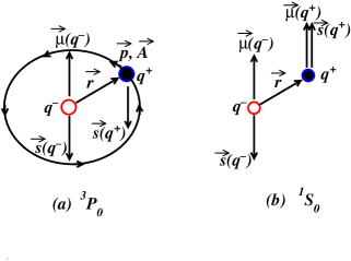
Figure 1: (a) The schematic picture of the ${}^{3}P_{0}$ state spin configuration and the orbital motion of a negative charge $q^{-}$ and a positive charge $q^{+}$ that can lead to a strong magnetic attraction at short distances. Here, ${\hbox{\boldmath${\mu}$}}(q^{\pm})$ is the magnetic moment of the charge $q^{\pm}$ arising from its spin $\hbox{\boldmath${s}$}(q^{\pm})$. (b) The schematic picture of the spin configurations of $q^{-}$ and $q^{+}$ in the ${}^{1}S_{0}$ state.

Previously, one of us (CYW), in collaboration with R. L. Becker, studied the $(e^{+}e^{-})$ system using the Kemmer-Fermi-Yang equation Kem37 with interactions consisting of the Coulomb interaction and the vector (magnetic) interaction, ${\hbox{\boldmath${A}$}}_{i}={\hbox{\boldmath${\mu}$}}_{j}\times({\hbox{\boldmath${r}$}}_{i}-{\hbox{\boldmath${r}$}}_{j})/|{\hbox{\boldmath${r}$}}_{i}-{\hbox{\boldmath${r}$}}_{j}|^{3}$, in connection with a possible scalar ${}^{3}P_{0}$ magnetic resonance Won86 . The interest was to investigate whether there could be a resonance at the mass of 1.579 MeV that might explain the anomalous positron peak in heavy-ion collisions near the Coulomb barrier Sch83 . The experimental evidence for the anomalous positron peak later turned out to be negative when greater statistics were accumulated Ahm95 . Nevertheless, it remains of interest to study the behavior of the two-body system at short distances and see how the attractive magnetic interaction in the ${}^{3}P_{0}$ state may reveal itself in some observable properties.

While the use of the Kemmer-Fermi-Yang equation with a two-body magnetic interaction is useful to motivate an approximate description Won86 , a consistent relativistic description of the two-body interaction at short distances can be found in the relativistic two body Dirac equations (TBDE) formulated in Dirac’s constraint dynamics dirac ; cnstr ; cra82 ; cww . These relativistic two body Dirac equations give a good description to the entire meson mass spectrum (excluding most flavor-mixed mesons) with constituent world-scalar and vector potentials depending on just two or three invariant functions, in previous relativistic quark-model calculations crater2 ; tmlk ; unusual .

The application of the TBDE equations to two-body bound and resonance states in quantum electrodynamics has intrinsic merits. In Ref. bckr , the properties of these TBDE equations that made them work so well for the relativistic quark model were investigated by solving them nonperturbatively (i.e. analytically or numerically) in quantum electrodynamics (QED), where order $\alpha^{4}$ perturbative solutions are well known. The two coupled Dirac equations in the constraint formalism depend on Lorentz-covariant potentials between the two constituents and act on a 16-component wave function. An exact Pauli reduction led to a second-order relativistic Schrödinger-like equation for a reduced four-component wave function with an effective interaction containing all the dependencies on spin, orbital angular momentum, and tensor operators. We were able to solve the TBDE nonperturbatively (analytically or numerically) as well as perturbatively because the spin dependent short-distance components of the effective interaction are not singular cww ; bckr . The situation is very different from the approximate Fermi-Breit forms, which contain singular potentials and necessitate the introduction of arbitrary short-distance cut-off parameters. The spin dependence of the relativistic potentials in the exact Schrödinger-like equation arises naturally from the relativistic reduction procedure and it incorporates detailed minimal interaction and dynamical recoil effects, characteristic of field theory. We shall also use the term “quasipotential” to represent this effective, non-singular interaction.

To obtain the interaction used in the TBDE formalism, we first determined the relativistic quasipotential to the lowest order in $\alpha$ for the Schr ödinger-like equation in Ref. bckr by comparing the effective interaction with the interaction derived from the Bethe-Salpeter equation. This, in turn led to an invariant Coulomb-like potential $A(r)=-\alpha/r$, where $\alpha$ is the coupling constant. Insertion of this information into the minimal interaction structures of the two body Dirac equations then completely determined all aspects (spin-dependent as well as spin-independent) of the interaction. (In decay we gave a procedure to construct the full 16-component solution to our coupled first-order Dirac equations from a solution of the second-order equation for the reduced wave function.)

Next, we showed that both the quantum mechanical perturbative and the TBDE non-perturbative treatments (i.e. analytic or numerical) yield the standard spectral results for QED and related interactions through order $\alpha^{4}$ . Such an agreement depends crucially on the inclusion of the coupling between various components of our 16-component Dirac wave functions and on the short-distance behavior of the relativistic quasipotential in the associated Schrödinger-like equation. We then examined the speculations Won86 whether the quasipotentials (including the angular momentum barrier) for some states in the $e^{+}e^{-}$ system may become attractive enough at short distances to yield a pure QED resonance corresponding to the anomalous positron peaks in heavy-ion collisions Sch83 . For the ${}^{3}P_{0}$ state we found that, even though the quasipotential becomes attractive and overwhelms the centrifugal barrier at short distances, the spatial extension of the attraction is not large enough to hold a resonance at the energy of 1.579 MeV bckr . This result contradicted predictions of such states by other authors Spe91 based on numerical solutions of three-dimensional truncations of the Bethe-Salpeter equation, for which the entire QED bound state spectrum has been treated successfully through order $\alpha^{4}$ only by perturbation theory.

In this paper we return to this problem of the magnetic resonance and magnetic states, not motivated so much by new experimental data as by a discovery of an additional peculiar solution of the TBDE overlooked in the earlier work in Ref. bckr . Our examination of the two body Dirac equations reveals that at short distance for both ${}^{1}S_{0}$ and ${}^{3}P_{0}$ states, the magnetic interactions is indeed quite strong. As a consequence, they counterbalance other repulsive interactions to result in a quasipotential for these states that behaves as $-\alpha^{2}/r^{2}$ at short distances.

In standard quantum mechanics for central interactions including the angular momentum barrier $L(L+1)/r^{2}$ for states with $L\neq 0$ at short distances, one generally retains only one of the two solutions for the radial part of the wave function, $u=r\psi$, the one that grows with distance as ($\sim r^{L+1})$, dropping the other solution($\sim r^{-L})$ as being too singular. If we likewise represent the quasipotential as $\lambda(\lambda+1)/r^{2}$ with $\lambda=(-1+\sqrt{(1-4\alpha^{2}})/2$, it leads to a short-distance solution that behaves as $r^{\lambda+1}$, which we call the usual solution, in addition to a solution, whose radial part grows as $r^{-\lambda}$, which we call the peculiar solution. However, both usual and peculiar states have quantum-mechanically acceptable behaviors at short distances, as the wave functions at short-distances are square-integrable.

In the case of the spin singlet ${}^{1}S_{0}$ states, the eigenstates and eigenenergies can be obtained analytically and are found to encompass both usual and peculiar states. We find usual bound states with attributes the same as those one usually encounters in QED and QCD, explicitly agreeing with the standard perturbative results through order $\alpha^{4}$. In contrast, the peculiar ${}^{1}S_{0}$ ground state of a fermion-antifermion pair with a fermion rest mass $m$ has a root-mean-square radius approximately $1/m$, a binding energies approximately $B_{p}$$\sim$$(2-\sqrt{2})m$, and a rest mass approximately $\sqrt{2}m$. However, the $(n+1)$ th ${}^{1}S_{0}$ peculiar state is nearly degenerate in energy and approximately equal in size with the $n$th usual ${}^{1}S_{0}$.

The existence of both usual and peculiar eigenstates in the same system brings with them conceptual and mathematical problems of the non-self-adjoint property of the mass operator and the over-completeness of the set of eigenstates. We resolve these problems by the introduction of a new quantum number, the peculiarity quantum number, that makes the mass operator self-adjoint and the combined set of usual and peculiar states a complete set in an enlarged Hilbert space.

In the case of the ${}^{3}P_{0}$ states, both of the usual and peculiar solutions reflect the overwhelmed centrifugal barrier and so differ substantially from the $r^{L+1}$ and $r^{-L}$ behaviors at short distances respectively. As a peculiar state radial wave function $u$ rises from the zero value at the origin as $r^{-\lambda}\sim r^{\alpha^{2}}$, the strongly attractive magnetic interaction has the tendency of bending the wave function in such a way to allow for the possibility of a resonance. Furthermore, as the quasipotential obtained through the relativistic reduction is sensitively energy dependent, we can explore the behavior of the two-body system over a larger domain of energies. We find that the usual solutions lead to no resonant behavior, but the peculiar solution can lead to a ${}^{3}P_{0}$ resonance whose phase shift changes by $\pi$ at an appropriate energy, depending on the description of the internal structure of the charges, the mass of the constituent, and the coupling constant.

This paper is organized as follows. In Sec. II we give a review of the two body Dirac equations of constraint dynamics.  For those readers who are already familiar with the constraint approach we refer them to the TBDE given in Eq. (14) and their Schrödinger-like Pauli reduction given in Eq. (17). We specialize to electromagnetic-like interactions only in this paper. We give in Sec. III the single-component radial forms of Eq. (17) relevant to this paper. In Sec. IV we examine both solutions for the ${}^{1}S_{0}$ states. In addition to examining new bound state solutions, we show how the ${}^{1}S_{0}$ wave functions for positive energies (and their corresponding phase shifts) can be determined analytically in terms of Coulomb wave functions for noninteger angular momentum. This is done for both the usual and peculiar solutions. We explain why and how we introduce of a new quantum number, which we call the peculiarity quantum number, to solve the problems of the non-self-adjoint property of the mass operator and the over-completeness of the set of eigenstates. In Sections V we examine the short distance behaviors for the ${}^{3}P_{0}$ state for the usual  and peculiar solutions. In Sec. VI we discuss the variable phase shift formalism of Calogero cal and outline how we use it for our phase shift analysis.  Since the short distance behavior of the ${}^{3}P_{0}$ quasipotential is the same as that of ${}^{1}S_{0}$ quasipotential, we can use those same ${}^{1}S_{0}$ Coulomb wave functions as reference wave functions in that region to compute phase shifts.  There is, however, an additional term (proportional to $\delta({\hbox{\boldmath${r}$})}$) that does not appear in the extreme short distance region for the ${}^{1}S_{0}$ quasipotential. Even though this term does not contribute in the case of the phase shift for the usual solution, its contribution to the phase shift calculations for the peculiar solution must be considered. In Sec. VI we discuss our numerical results and in Sec. VII our conclusions. Various technical results are presented in the appendices. In Appendix A we give an outline of the details on the relation between the two-body Dirac equations and their Pauli reduced Schrödinger forms. In Appendix B we present the radial forms of those Schrödinger-like equations for a general angular momentum coupling. In Appendix C we present details of the ${}^{1}S_{0}$ usual and peculiar bound states.  In Appendix D we review the connections between the Coulomb wave functions for noninteger angular momentum index.  Appendix E presents a review of the variable phase method of Calogero cal for our problem.

II TWO BODY DIRAC EQUATIONS

We briefly review the two body Dirac equations of constraint dynamics cra82 ; cww ; crater2 ; tmlk ; unusual ; saz86 providing a covariant three dimensional truncation of the Bethe Salpeter equation for the two body system.  Sazdjian saz85 ; saz92 ; saz97 has shown that the Bethe-Salpeter equation can be algebraically transformed into two independent equations. The first yields a covariant three dimensional eigenvalue equation which for spinless particles takes the form

$$\biggl{(}\mathcal{H}_{10}+\mathcal{H}_{20}+2\Phi\biggr{)}\Psi(x_{1},x_{2})=0,$$ (1)

where $\mathcal{H}_{i0}=p_{i}^{2}+m_{i}^{2}$ . The quasipotential $\Phi$ is a modified geometric series in the Bethe-Salpeter kernel $K$ such that in lowest order in $K$

$$\Phi=\pi i\delta(P\cdot p)K,$$ (2)

where $P=p_{1}+p_{2}$ is the total momentum, $p=\mu_{2}p_{1}-\mu_{1}p_{2}$ is the relative momentum, $w$ is the invariant total center of momentum (c.m.) energy with $P^{2}=-w^{2}$.   The $\mu_{i}$ must be chosen so that the relative coordinate $x=x_{1}-x_{2}$ and $p$ are canonically conjugate, i.e. $\mu_{1}+\mu_{2}=1$. The second equation, Eq. (2), overcomes the difficulty of treating the relative time in the center of momentum system by setting an invariant condition on the relative momentum $p$,

$$(\mathcal{H}_{10}-\mathcal{H}_{20})\Psi(x_{1},x_{2})=0=2P\cdot p\Psi(x_{1},x_{2}).$$ (3)

Note that this implies $p^{\mu}\Psi=p_{\perp}^{\mu}\Psi\equiv(\eta^{\mu\nu}+\hat{P}^{\mu}\hat{P}^{\nu})p_{\nu}\Psi$ in which $\hat{P}^{\mu}=P^{\mu}/w$ is a time like unit vector $(\hat{P}^{2}=-1)$ in the direction of the total momentum.

One can further combine the sum and the difference of Eqs. (1) and (3) to obtain a set of two relativistic equations one for each particle with each equation specifying two generalized mass-shell constraints

$$\mathcal{H}_{i}\Psi(x_{1},x_{2})=(p_{i}^{2}+m_{i}^{2}+\Phi)\Psi(x_{1},x_{2})=0,~{}i=1,2,$$ (4)

including the interaction with the other particle. These constraint equations are just those of Dirac’s Hamiltonian constraint dynamics for spinless particles dirac ; cnstr ; cra84s . In order for Eq. (4) to have consistent solutions, Dirac’s constraint dynamics stipulate that these two constraints must be compatible among themselves, $[\mathcal{H}_{1},\mathcal{H}_{2}]\Psi=0$, that is, they must be first class constraints. This requires that the quasipotential $\Phi$ satisfy $[p_{1}^{2}-p_{2}^{2},\Phi]\Psi=0$. Working out the commutator shows that for this to be true in general, $\Phi$ must depend on the relative coordinate $x=x_{1}-x_{2}$ only through its component, $x_{\perp},$ perpendicular to $P,$

$$x_{\perp}^{\mu}=(\eta^{\mu\nu}+\hat{P}^{\mu}\hat{P}^{\nu})(x_{1}-x_{2})_{\nu}.$$ (5)

The invariant $x_{\perp}^{2}\equiv r^{2}$ becomes $\mathbf{r}^{2}$ in the c.m. frame. Since the total momentum is conserved, the single component wave function $\Psi~{}$in coordinate space is a product of a plane wave eigenstate of $P$ and an internal part $\psi(x_{\perp})$ cra87 .

We find a plausible structure for the quasipotential $\Phi$ by observing that the one-body Klein-Gordon equation $(p^{2}+m^{2})\psi=({\hbox{\boldmath${p}$}}^{2}-\varepsilon^{2}+m^{2})\psi=0$ takes the form $({\hbox{\boldmath${p}$}}^{2}-\varepsilon^{2}+m^{2}+2mS+S^{2}+2\varepsilon A-A^{2})\psi=0~{}$when one introduces a scalar interaction and time-like vector interaction via the minimum substitutions $m\rightarrow m+S~{}$and $\varepsilon\rightarrow\varepsilon-A$. In the two-body case, separate classical fw and quantum field theory saz97 arguments show that when one includes world scalar and vector interactions then $\Phi$ depends on two underlying invariant functions $S(r)$ and $A(r)$ ($r=\sqrt{x_{\perp}^{2}}$) through the two body Klein-Gordon-like potential form with the same general structure, that is

$$\Phi=2m_{w}S+S^{2}+2\varepsilon_{w}A-A^{2}.$$ (6)

Those field theories further yield the c.m. energy dependent forms

$$m_{w}=m_{1}m_{2}/w,$$ (7)

and

$$\varepsilon_{w}=(w^{2}-m_{1}^{2}-m_{2}^{2})/2w,$$ (8)

ones that Tododov cnstr ; tod71 introduced as the relativistic reduced mass and effective particle energy for the two-body system. Similar to what happens in the nonrelativistic two-body problem, in the relativistic case we have the motion of this effective particle taking place as if it were in an external field  (here generated by $S$ and $A$).  The two kinematical variables (7) and (8) are related to one another by the Einstein condition

$$\varepsilon_{w}^{2}-m_{w}^{2}=b^{2}(w),$$ (9)

where the invariant

$$b^{2}(w)\equiv(w^{4}-2w^{2}(m_{1}^{2}+m_{2}^{2})+(m_{1}^{2}-m_{2}^{2})^{2})/4w^{2},$$ (10)

is the c.m. value of the square of the relative momentum expressed as a function of $w$. One also has

$$b^{2}(w)=\varepsilon_{1}^{2}-m_{1}^{2}=\varepsilon_{2}^{2}-m_{2}^{2},$$ (11)

in which $\varepsilon_{1}$ and $\varepsilon_{2}$ are the invariant c.m. energies of the individual particles satisfying

$$\ \varepsilon_{1}+\varepsilon_{2}=w,\ \varepsilon_{1}-\varepsilon_{2}=(m_{1}^{2}-m_{2}^{2})/w.$$ (12)

In terms of these invariants, the relative momentum appearing in Eq. (2) and (3) is given by

$$p^{\mu}=(\varepsilon_{2}p_{1}^{\mu}-\varepsilon_{1}p_{2}^{\mu})/w\mathrm{,}$$ (13)

so that $\mu_{1}+\mu_{2}=(\varepsilon_{1}+\varepsilon_{2})/w=1$. In tod the forms for these two-body effective kinematic variables are given sound justifications based solely on relativistic kinematics, supplementing the dynamical arguments of fw and saz97 .

This covariant and useful three-dimensional truncation of the Bethe-Salpeter equation has been extended to the case of a two-fermion system where the two constraint equations become the two body Dirac equations (TBDE) cra82 ; cra82 ; cww ; crater2 ; tmlk ; unusual

$$\mathcal{S}_{1}\psi \equiv\gamma_{51}(\gamma_{1}\cdot(p_{1}-\tilde{A}_{1})+m_{1}+\tilde{S}_{1})\Psi=0,$$

$$\mathcal{S}_{2}\psi \equiv\gamma_{52}(\gamma_{2}\cdot(p_{2}-\tilde{A}_{2})+m_{2}+\tilde{S}_{2})\Psi=0.$$ (14)

Here $\Psi$ is a sixteen component wave function consisting of an external plane wave part that is an eigenstate of $P$ and an internal part $\psi=\psi(x_{\perp})$. The vector potential$\ \tilde{A}_{i}^{\mu}$ was taken to be an electromagnetic-like four-vector potential with the time-like and space-like portions both arising from a single invariant function $A(r)$. The tilde on these four-vector potentials indicate that they are not only position dependent but also spin dependent by way of the gamma matrices. The operators $\mathcal{S}_{1}$ and $\mathcal{S}_{2}$ must commute or at the very least $[\mathcal{S}_{1},\mathcal{S}_{2}]\psi=0$ since they operate on the same wave function. This compatibility condition gives restrictions on the spin dependencies of the vector and scalar potentials,

$$\tilde{A}_{i}^{\mu}=\tilde{A}_{i}^{\mu}(A(r),p_{\perp},\hat{P},w,\gamma_{1},\gamma_{2}),$$ (15)

in addition to requiring that they depend on the invariant separation $r\equiv\sqrt{x_{\perp}^{2}}$ through the invariant $A(r)$. The covariant constraint (3) can also be shown to follow from Eq. (14). We give the explicit connections between $\tilde{A}_{i}^{\mu}$ and the invariant $A(r)$ in Appendix A. (A similar dependence occurs for $\tilde{S}_{i}$ on $S(r).$)  The general structural dependence on $A(r)$ and $S(r)$ and the spin dependence of $\tilde{A}_{i}^{\mu},\tilde{S}_{i}$ is a consequence of the compatibility condition $[\mathcal{S}_{1},\mathcal{S}_{2}]\psi=0.$

The Pauli reduction of these coupled Dirac equations lead to a covariant Schr ödinger-like equation for the relative motion with an explicit spin-dependent potential $\Phi$,

$${\bigg{(}}p_{\perp}^{2}+\Phi(S(r),A(r),p_{\perp},\hat{P},w,\sigma_{1},\sigma_{2}){\bigg{)}}\psi_{+}=b^{2}(w)\psi_{+},$$ (16)

with $b^{2}(w)$ playing the role of the eigenvalue. This eigenvalue equation can then be solved for the four-component effective particle spinor wave function $\psi_{+}$ related to the sixteen component spinor $\psi(x_{\perp})$ in appendix A.

In Appendix A we outline the steps needed to obtain the explicit c.m. form of Eq. (16). That form is liu , saz94 , crater2 ; tmlk ; unusual

$$\{ {\hbox{\boldmath${p}$}}^{2}+\Phi({\hbox{\boldmath${r}$},}m_{1},m_{2},w,{\hbox{\boldmath${\sigma}$}}_{1},{\hbox{\boldmath${\sigma}$}}_{2})~{}\}\psi_{+}$$ (17)

$$= \{{\hbox{\boldmath${p}$}}^{2}+2m_{w}S+S^{2}+2\varepsilon_{w}A-A^{2}+\Phi_{D}$$

$$+{\hbox{\boldmath${L}$}\cdot(\hbox{\boldmath${\sigma}$}}_{1}{+\hbox{\boldmath${\sigma}$}}_{2}{)}\Phi_{SO}+{\hbox{\boldmath${\sigma}$}}_{1}{\hbox{\boldmath${\cdot}$}\hat{r}\sigma}_{2}{\hbox{\boldmath${\cdot}$}\hat{r}L\cdot(\sigma}_{1}{\hbox{\boldmath${+}$}\sigma}_{2}{\hbox{\boldmath${)}$}}\Phi_{SOT}$$

$$+{\hbox{\boldmath${\sigma}$}}_{1}{\hbox{\boldmath${\cdot}$}\sigma}_{2}\Phi_{SS}+(3{\hbox{\boldmath${\sigma}$}}_{1}{\hbox{\boldmath${\cdot}$}\hat{r}\sigma}_{2}{\hbox{\boldmath${\ }$}\cdot\hat{r}-\hbox{\boldmath${\sigma}$}}_{1}{\hbox{\boldmath${\cdot}$}\sigma}_{2})\Phi_{T}$$

$$+{\hbox{\boldmath${L}$}\cdot(\sigma}_{1}{\hbox{\boldmath${-}$}\sigma}_{2}{\hbox{\boldmath${)}$}\Phi}_{SOD}+i{\hbox{\boldmath${L}$}\cdot\sigma}_{1}{\hbox{\boldmath${\times}$}\sigma}_{2}\Phi_{SOX}\}\psi_{+}$$

$$= b^{2}\psi_{+},$$

where the detailed forms of the separate quasipotentials $\Phi_{i}$ are given in Appendix A. The subscripts of most of the quasipotentials are self explanatory.  After the eigenvalue $b^{2}$ of (17) is obtained, the invariant mass of the composite two-body system $w$ can then be obtained by inverting Eq. (10). It is given explicitly by

$$w=\sqrt{b^{2}+m_{1}^{2}}+\sqrt{b^{2}+m_{2}^{2}}.$$ (18)

For this reason we call the operator that appears to the left of Eq. (17) the invariant mass operator. The structure of the linear and quadratic terms in Eq. (17) as well as the Darwin and spin-orbit terms, are plausible in light of the discussion given above Eq. (6), and in light of the static limit Dirac structures that come about from the Pauli reduction of the Dirac equation. Their appearance as well as that of the remaining spin structures are direct outcomes of the Pauli reductions of the simultaneous TBDE Eq. (14). In this paper we take the scalar interaction $S(r)=0$.

III TBDE SINGLE COMPONENT WAVE EQUATIONS.

The 4 component two-body wave function $\psi_{+}$ of the above Pauli-form ( 17) of the TBDE can be conveniently represented by spin-singlet $S=0$ and spin-triplet $S=1$ components with quantum numbers $\{J,L,S\}$ and basis wave functions

$$\langle{\hbox{\boldmath${r}$}}|wJLS\rangle\equiv\psi_{JLS}({\hbox{\boldmath${r}$}})=\frac{u_{JLS}(r)}{r}Y_{JM}(\mathbf{\hat{r})}.$$ (19)

In general, the singlet and triplet states are coupled. However, we see from Appendix B that for the case of equal masses and certain angular momentum states, the spin singlet and spin triplet components decouple, and the TBDE reduce to a single component equation.

Specifically, for the spin-singlet $S=0$ state with $J=L$, (the ${}^{1}J_{J}$ state), the TBDE is

$$\{-\frac{d^{2}}{dr^{2}}+\frac{J(J+1)}{r^{2}}+2\varepsilon_{w}A-A^{2}+\Phi_{D}{-}3\Phi_{SS}\}u_{JJ0}=b^{2}u_{JJ0},$$ (20)

where, using the results in Appendix B, the magnetic interaction $-3\Phi_{SS}$ is

$$-3\Phi_{SS} = -3\Phi_{SS}(A,A^{\prime},{\nabla}^{2}A)=-3(\frac{1}{r^{2}}-\frac{3}{2r}\left(\frac{A^{\prime}}{w-2A}\right))((\frac{1}{\sqrt{1-2A/w}}+\sqrt{1-2A/w})-2)$$

$$-\frac{3}{2r}\left(\frac{A^{\prime}}{w-2A}\right)(\frac{1}{\sqrt{1-2A/w}}-\sqrt{1-2A/w})\mathcal{-}\frac{21}{2}\left(\frac{A^{\prime}}{w-2A}\right)^{2}-\frac{3{\hbox{\boldmath${\nabla}$}}^{2}A}{w-2A}$$

$$= -\Phi_{D}(A,A^{\prime},{\nabla}^{2}A),$$

which is attractive and singular, as we discussed in the Introduction. At large distances and for $A=-\alpha/r$ potential, ${\hbox{\boldmath${\nabla}$}}^{2}A=4\pi\alpha\delta({\hbox{\boldmath${r}$}})$ and the spin-spin interaction indeed becomes a singular interaction as described in Jac62 . In addition to the magnetic spin-spin interaction, there is also the repulsive Darwin quasipotential $\Phi_{D}$.  In the ${}^{1}J_{J}$ state, the attractive magnetic spin-spin quasipotential in the spin-singlet configuration exactly cancels the repulsive Darwin quasipotential,

$${-}3\Phi_{SS}+\Phi_{D}=0.$$ (22)

As a result of this remarkable cancellation, the eigenvalue equation for the ${}^{1}J_{J}$ state in Eq. (III) becomes simply

$$\{-\frac{d^{2}}{dr^{2}}+\frac{J(J+1)}{r^{2}}+2\varepsilon_{w}A-A^{2}\}u_{JJ0}=b^{2}u_{JJ0}.$$ (23)

Of all spin-singlet states, only in the ${}^{1}S_{0}$ states ($J=L=0)$ do the effects of the quasipotential and the absence of a centrifugal barrier make the combined quasipotential strongly attractive at short-distances. This, of course, would not happen were it not for the highly attractive spin-spin interaction discussed in the Introduction and in Eq. (III). Among the spin-singlet states with different $J$ quantum numbers, we shall therefore focus our attention only on the ${}^{1}S_{0}$ states.

For the spin-triplet $S=1$ states, there are two states with single component radial equations. The first is the ${}^{3}J_{J}$ state whose radial equation takes the form ($J\geq 1$)

$$\{-\frac{d^{2}}{dr^{2}}+\frac{J(J+1)}{r^{2}}+2\varepsilon_{w}A-A^{2}-\frac{2A^{\prime}}{r\left(w-2A\right)}+3\left(\frac{A^{\prime}}{w-2A}\right)^{2}+\frac{{\hbox{\boldmath${\nabla}$}}^{2}A}{w-2A}\}u_{J1J}=b^{2}u_{JJ1}.$$ (24)

The second is the ${}^{3}P_{0}$ equation which takes the form

$$\{-\frac{d^{2}}{dr^{2}}+\frac{2}{r^{2}}+2\varepsilon_{w}A-A^{2}-\frac{8A^{\prime}}{r\left(w-2A\right)}+8\left(\frac{A^{\prime}}{w-2A}\right)^{2}+\frac{2{\hbox{\boldmath${\nabla}$}}^{2}A}{w-2A}\}u_{011}=b^{2}u_{011}.$$ (25)

Of the two spin-triplet cases, only in the ${}^{3}P_{0}$ states ($J=0,$ $L=1)~{}$ do the combined effects of the quasipotentials become so strongly attractive at short-distances that they overwhelm the presence of the centrifugal barrier. As discussed in the Introduction, this is due to the highly attractive spin-orbit interaction (“magnetic” interaction) when the total spin and the orbital angular momentum are oppositely aligned. In that case, the competing effects of both the short-distance attraction and the presence of the potential barrier raise the question whether the attraction is strong enough to hold a resonance state in the continuum. Among the spin-triplet states with different $J$ and $L$ quantum numbers, we shall therefore focus our attention only on the ${}^{3}P_{0}$ states.

In the last term of the quasipotential in Eq. (25), the quantity $\nabla^{2}A$ is related to the particle charge density, $\rho(\hbox{\boldmath${r}$})$, seen by each of the two particles by

$$\nabla^{2}A(\hbox{\boldmath${r}$})=4\pi\alpha\rho(\hbox{\boldmath${r}$}).$$ (26)

Therefore, the equation for the two-body relative wave function for the ${}^{3}P_{0}$ state becomes

$$\biggl{\{}-\frac{d^{2}}{dr^{2}}+\frac{2}{r^{2}}+2\varepsilon_{w}A-A^{2}-\frac{8A^{\prime}}{r\left(w-2A\right)}+8\left(\frac{A^{\prime}}{w-2A}\right)^{2}+\frac{8\pi\alpha\rho(\hbox{\boldmath${r}$})}{w-2A}\biggr{\}}u_{011}=b^{2}u_{011}.$$ (27)

As we shall see in this case, the attractive magnetic interaction overwhelms the centrifugal barrier, allowing the wave function to reach the short-distance region where the particle charge density $\rho(r)$, if any, can be exposed for scrutiny. This is in contrast to the situation for states in which the centrifugal barrier dominates the short-distance region. In that case, the centrifugal barrier will prevent the wave function from reaching the short-distance region and the particle charge density will not make as a significant difference in observable quantities. We obtain the important result that the ${}^{3}P_{0}$ quasipotential depends explicitly on the particle charge density $\rho(\hbox{\boldmath${r}$})$ at short distances. As a consequence, some observable quantities may depend more critically on the nature of the particle charge distribution and the forces binding the charge elements together.

For the ${}^{3}P_{0}$ state, it is convenient to separate out the centrifugal barrier $2/r^{2}$ and the quasipotential $\Phi$ to write the above equation as

$$\biggl{\{}-\frac{d^{2}}{dr^{2}}+\frac{2}{r^{2}}+\Phi(\hbox{\boldmath${r}$})\biggr{\}}u_{011}=b^{2}u_{011},$$ (28)

where

$$\Phi(\hbox{\boldmath${r}$})=2\varepsilon_{w}A-A^{2}-\frac{8A^{\prime}}{r\left(w-2A\right)}+8\left(\frac{A^{\prime}}{w-2A}\right)^{2}+\frac{8\pi\alpha\rho(\hbox{\boldmath${r}$})}{w-2A}.$$ (29)

In our early work bckr , we limited our attention to energy regions around 1.579 MeV for the $(e^{+}e^{-})$ system and searched for ${}^{3}P_{0}$ resonances whose wave functions start from the origin in the usual way. We found no resonance states. We return to this problem again including now an additional (peculiar) solution of the TBDE that was overlooked in the earlier work but has quantum-mechanically acceptable behaviors at short distances.

In Eqs. (27)), both the gauge field $A(r)$ and the gauge field source $\rho(r)$ appear in the equation of motion for the wave function in the ${}^{3}P_{0}$ state. The appearance of the fermion charge source distribution $\rho(r)$ brings into focus the question whether it is sufficient to describe the magnetic interaction in the ${}^{3}P_{0}$ state completely within quantum electrodynamics or quantum chromodynamics. Electrons in QED and quarks in QCD are taken to be point particles with no structure. It may be necessary to go beyond these field theories, to include additional auxiliary interactions that hold the charge elements together, in order to properly describe the internal structure of these particles. If these auxiliary interactions act on the charged elements of the fermion to hold them together, they can also act on the charged elements of the antifermion charge and will affect the ${}^{3}P_{0}$ wave function in the interior region of the charge distribution $\rho(r)$.

The nature of these auxiliary forces holding the charged elements together is completely unknown, although there have been many attempts to carry out such an investigation. For example, in the Dirac’s model of an electron, a surface tension from an unknown axillary interaction is invoked to hold the electric charged elements of an electron together Dir48 ; Dir51 ; Dir52 ; Dir53 ; Dir62 ; Dir65 . However, our knowledge on the internal structures of electrons and quarks remain very uncertain. We shall return to examine how such a lack of knowledge of the internal structures of these elementary quanta leads to uncertainties in the ${}^{3}P_{0}$ magnetic resonance states in Sec. VC.

IV SOLUTIONS OF THE TWO BODY DIRAC EQUATIONS FOR THE ${}^{1}S_{0}$ STATE

IV.1 The ${}^{1}S_{0}$ quasipotential

We first consider the case of the ${}^{1}S_{0}$ state of a point fermion-antifermion pair with electric or color charges interact through an electromagnetic-type interaction arising from the exchange of a single photon or gluon. The single photon annihilation diagram does not contribute because the ${}^{1}S_{0}$ state is a charge parity even state. We thus have

$$A=-\frac{\alpha}{r}.$$ (30)

For brevity of notation in this subsection, we shall abbreviate the radial wave function $u_{0JJ}$=$u_{000}$ as $u$. Equation  (20) for $u$ becomes

$$\left\{-\frac{d^{2}}{dr^{2}}-\frac{2\varepsilon_{w}\alpha}{r}-\frac{\alpha^{2}}{r^{2}}\right\}u=b^{2}u.$$ (31)

with a short distance ($r<<\alpha/2\varepsilon_{w})$ behavior given by

$$\left\{-\frac{d^{2}}{dr^{2}}-\frac{\alpha^{2}}{r^{2}}\right\}u=0,$$ (32)

with solutions

$$u_{+} \sim r^{\lambda+1},$$

$$u_{-} \sim r^{-\lambda},$$

$$\lambda = (-1+\sqrt{1-4\alpha^{2}})/2,$$ (33)

or

$$u_{\pm}\sim r^{(1\pm\sqrt{1-4a^{2}})/2},$$ (34)

both of which approach zero as $r$ approaches zero. With these behaviors, the probability

$$\psi_{\pm}^{2}d^{3}r=\frac{u_{\pm}^{2}}{r^{2}}r^{2}drd\Omega=u_{\pm}^{2}drd\Omega=r^{(1\pm\sqrt{1-4a^{2}})}drd\Omega,$$ (35)

is finite for both signs. We call $u_{+}$ the usual solution, and it behaves as $r^{\lambda+1}\sim r^{1-\alpha^{2}}$ for small $\alpha$. We call $u_{-}$ the peculiar solution, and it behaves as $r^{-\lambda}\sim r^{\alpha^{2}}$for small $\alpha$. Both of these behaviors are physically acceptable near the origin in the sense of (i) $u(0)$$\rightarrow 0$, and (ii) being square-integrable in the neighborhood of $r\sim 0$.   We note that if the sign in front of $\alpha^{2}$ were positive or if we had non-zero angular momentum such that $L(L+1)-\alpha^{2}>0$ then the second or peculiar set of solutions are not physically admissible states.

In khel one finds a thorough discussion on the proper boundary condition for the radial wave function of the Schrödinger equation at the origin. They discuss several conditions that appear in the literature: (1) Continuity of $R=u/r$ at $r=0,$ requiring $u(0)=0$. (2) A finite differential probability in the spherical slice $(r,r+dr$), that is $R^{2}r^{2}dr<\infty$ requiring $u(r)\rightarrow r^{s+1},s>-1$ and again $u(0)=0$. (3) Requiring a finite total probability inside a sphere of small radius $a$ which allows a more singular behavior, namely $u(r)\rightarrow r^{-1/2+\varepsilon}$ where $\varepsilon>0$ is a small positive constant, which would also include a finite behavior of the norm. (4) Requiring time independence of the norm leading to $u(r)\rightarrow cr^{-s+1}$, $s<1$ which again leads to $u(0)=0.$ Reference khel furthermore shows that the radial Schrödinger equation [$-d^{2}/dr^{2}+l(l+1)/r^{2}+2mV(r)]u(r)=2mEu(r)$ is compatible with the full Schrödinger equation ($-\nabla^{2}+2mV(r))\frac{u(r)}{r}Y_{lm}=2mE\frac{u(r)}{r}Y_{lm}$ if and only if the condition$~{}u(0)=0$ is satisfied. This $u(0)=0$ condition is clearly satisfied for both solutions in Eq. (34).

In Schiff’s Quantum Mechanics schiff , a solution similar to the peculiar one discussed here is examined for the case of the Klein-Gordon equation for the Coulomb system. He argues that what we call the peculiar solution can be discarded since the source of the Coulomb attraction is a finite sized nucleus of radius $r_{0}$. In particular, he states that for $r<r_{0}$ for which the potential is finite all the way to the origin, matching at $r_{0}$ would rule out the peculiar solution. In our case, with point particles, the potential does not satisfy this condition.

IV.1.1 ${}^{1}S_{0}$ Bound States

The solutions of the ${}^{1}S_{0}$ bound states can be obtained analytically. In Appendix C we show how we can obtain the two sets of ${}^{1}S_{0}$ bound state solutions that correspond to the usual and peculiar short distance behaviors. The respective sets of eigenvalues and normalized eigenfunctions for the state with total invariant c.m. energy (mass) $w_{\pm n}$ and the principle quantum number $n$ is

$$w_{\pm n} = m\sqrt{2+2/\sqrt{1+{\alpha^{2}}/{(}n\pm\sqrt{1/4-\alpha^{2}}-1/2{)^{2}}}},$$

$$u_{\pm n}(r) = \left[\left(\frac{4\varepsilon_{w_{\pm}}\alpha r}{n_{\pm}^{\prime}}\right)^{2}\frac{n_{r}!}{2n_{\pm}^{\prime}(n_{\pm}^{\prime}+\lambda_{\pm})!}\right]^{1/2}\exp(-\frac{\varepsilon_{w_{\pm}}\alpha r}{n_{\pm}^{\prime}})\left(\frac{2\varepsilon_{w_{\pm}}\alpha r}{n_{\pm}^{\prime}}\right)^{\lambda_{\pm}+1}L_{n_{r}}^{2\lambda_{\pm}+1}(\frac{2\varepsilon_{w_{\pm}}\alpha r}{n_{\pm}^{\prime}}),$$ (36)

where $n_{\pm}^{\prime}=n_{r}+\lambda_{\pm}+1=n+\lambda_{\pm}$ and

$$\varepsilon_{w_{\pm}}=(w_{\pm}^{2}-2m^{2})/2w_{\pm}.$$ (37)

For the usual states $u_{+n}$, the bound state eigenvalues $w_{+n}$ agree with standard QED perturbative results through order $\alpha^{4}$,

$$w_{+n}=2m-m{\alpha^{2}}/{4}n^{2}-m\alpha^{4}/2n^{3}(1-11/32/n)+O(\alpha^{6}),~{}n=1,2,3,...$$ (38)

For the set of peculiar states $u_{-n}$, note that the peculiar ground state $u_{-1}$ with $n=1$ has eigenenergy (mass)

$$w_{-1}=m\sqrt{2+2/\sqrt{1+{\alpha^{2}}/({1/2}-\sqrt{1/4-\alpha^{2}}{)^{2}}}}\sim\sqrt{2}m\sqrt{1+\alpha},$$ (39)

which represents very tight binding, with a binding energy on the order 300 keV for an $e^{+}e^{-}$ state and a root-mean-square radius on the order of a Compton wave length instead of an angstrom. In particular we find (see Appendix C)

$$\sqrt{\langle r^{2}\rangle_{-1}}\rightarrow\frac{1}{m}.$$ (40)

We note further the anti-intuitive behavior of the peculiar ground state energy (mass), increasing with increasing coupling constant $\alpha$ instead of decreasing. The excited states are quite near to the usual bound states. We find the following pattern for those excited peculiar states

$$w_{-n}=2m-m{\alpha^{2}}/{4(}n-1)^{2}+m\alpha^{4}/2(n-1)^{3}\left(1+11/32(n-1)\right)+O(\alpha^{6});\text{ }n=2,3,4,...$$ (41)

In the nonrelativistic limit, where terms of order $\alpha^{4}$ are ignored we find that the states are degenerate with the $n$th usual state identical to the $(n+1)$th peculiar state.  If  we include the $\alpha^{4}$ corrections then we find that

$$w_{+n}-w_{-(n+1)}=-m\alpha^{4}/n^{3}.$$ (42)

  For all of the usual states and the remaining peculiar states we have

$$\langle r^{2}\rangle_{+n} = \frac{(n+\lambda_{+})^{2}}{6\left(\varepsilon_{w_{+n}}\alpha\right)^{2}}[(n+\lambda_{+})^{2}+5\alpha^{2}+3]\text{,~{}}n=1,2,3...,$$

$$\langle r^{2}\rangle_{-n} = \frac{(n+\lambda_{-})^{2}}{6\left(\varepsilon_{w_{-n}}\alpha\right)^{2}}[(n+\lambda_{-})^{2}+5\alpha^{2}+3]\text{,~{}}n=2,3...,$$ (43)

so that the size in the $(n+1)$th peculiar state is nearly the same as with the $n$th usual state.

As shown in the Appendix C, the two sets of solutions, are not orthogonal with respect to one another.  For example, the two $n=1$ wave functions have the respective forms

$$u_{+}(r) = c_{+}r^{\lambda_{+}+1}\exp(-\kappa_{+}\varepsilon_{w_{+}}\alpha r),$$

$$\kappa_{+} = \frac{2}{1+\sqrt{1-4\alpha^{2}}}=\frac{1}{\lambda_{+}+1},$$

$$u_{-}(r) = c_{-}r^{\lambda_{-}+1}\exp(-\kappa_{-}\varepsilon_{w_{-}}\alpha r),$$

$$\kappa_{-} = \frac{2}{1-\sqrt{1-4\alpha^{2}}}=\frac{1}{\lambda_{-}+1},$$ (44)

where for brevity of notation, we have omitted the principal quantum number designation in $u\pm$ for the of the ground state. Clearly since they are both zero node solutions we have

$$\langle u_{-}|u_{+}\rangle=\int_{0}^{\infty}dru_{+}(r)u_{-}(r)\neq 0.$$ (45)

How do we reconcile this with the expected orthogonality of the eigenfunctions of a self-adjoint operator corresponding to different eigenvalues. In the present context, the naive self-adjoint property requires that

$$\langle u_{+}|(-\frac{d^{2}}{dx^{2}}-\frac{2}{x}-\frac{\alpha^{2}}{x^{2}})|u_{-}\rangle=\langle u_{-}|(-\frac{d^{2}}{dx^{2}}-\frac{2}{x}-\frac{\alpha^{2}}{x^{2}})|u_{+}\rangle.$$ (46)

This boils down to

$$\int_{0}^{\infty}dxu_{+}\frac{d^{2}u_{-}}{dx^{2}}=\int_{0}^{\infty}dxu_{-}\frac{d^{2}u_{+}}{dx^{2}}.$$ (47)

Let us integrate by parts.   Then we have

$$\int_{0}^{\infty}dxu_{+}\frac{d^{2}u_{-}}{dx^{2}} = \left(u_{+}\frac{du_{-}}{dx}\right)\biggr{|}_{0}^{\infty}-\int_{0}^{\infty}dx\frac{du_{+}}{dx}\frac{du_{-}}{dx}$$

$$= \left(u_{-}\frac{du_{+}}{dx}\right)\biggr{|}_{0}^{\infty}-\int_{0}^{\infty}dx\frac{du_{+}}{dx}\frac{du_{-}}{dx}.$$

We thus have a self-adjoint operator if

$$\left(u_{+}\frac{du_{-}}{dx}\right)\biggr{|}_{0}^{\infty}=\left(u_{-}\frac{du_{+}}{dx}\right)\biggr{|}_{0}^{\infty}.$$ (49)

Now clearly these vanish at the upper end points.  Since we have that

$$\frac{du_{+}}{dx} = u_{+}(\frac{\lambda_{+}+1}{x}-\frac{1}{\lambda_{+}+1}),$$

$$\frac{du_{-}}{dx} = u_{-}(\frac{\lambda_{-}+1}{x}-\frac{1}{\lambda_{-}+1}).$$ (50)

at the lower end point the LHS of Eq. (49) is

$$\underset{x\rightarrow 0}{\lim}x^{\lambda_{+}+1}\exp(-x/(\lambda_{+}+1))x^{\lambda_{-}+1}\exp(-x/(\lambda_{-}+1))(\frac{\lambda_{-}+1}{x}-\frac{1}{\lambda_{-}+1})$$ (51)

$$= \underset{x\rightarrow 0}{\lim}x(\frac{\lambda_{-}+1}{x}-\frac{1}{\lambda_{-}+1})=\lambda_{-}+1$$

whereas at the lower end point the RHS is $\lambda_{+}+1\neq\lambda_{-}+1$. Thus, the second derivative is not self-adjoint in this context! This accounts for the non-orthogonality of the usual and peculiar ground states in Eq. (45).

In general beginning with a set of usual and peculiar wave functions $\{u_{+n},u_{-n}\}$ such that

$$\langle u_{+n}|u_{+n^{\prime}}\rangle = \delta_{nn^{\prime}},$$

$$\langle u_{-n}|u_{-n^{\prime}}\rangle = \delta_{nn^{\prime}},$$

$$\langle u_{-n}|u_{+n}\rangle \equiv b_{nn^{\prime}}=b_{n^{\prime}n},$$ (52)

we find with

$$H \equiv \frac{1}{\left(\varepsilon_{w}\alpha\right)^{2}}\left[-\frac{d^{2}}{dr^{2}}-\frac{2\varepsilon_{w}\alpha}{r}-\frac{\alpha^{2}}{r^{2}}\right]=\left[-\frac{d^{2}}{dx^{2}}-\frac{2}{x}-\frac{\alpha^{2}}{x^{2}}\right],$$

$$Hu_{\pm n} = h_{\pm n}u_{\pm n},$$

$$h_{\pm n} \equiv -\kappa_{\pm n}^{2}=-1/(\lambda_{\pm}+n)^{2},~{}n=1,2,...$$ (53)

where $x=\varepsilon_{w}\alpha r$, that

$$\langle u_{+n}|H|u_{+n^{\prime}}\rangle = \delta_{nn^{\prime}}h_{+n}$$

$$\langle u_{-n}|H|u_{-n^{\prime}}\rangle = \delta_{nn^{\prime}}h_{-n},$$

$$\langle u_{-n}|H|u_{+n^{\prime}}\rangle = b_{nn^{\prime}}h_{+n^{\prime}}$$

$$\langle u_{+n}|H|u_{-n^{\prime}}\rangle = b_{nn^{\prime}}h_{-n^{\prime}}\neq\langle u_{-n^{\prime}}|H|u_{+n}\rangle.$$ (54)

In the first two terms it does not matter whether the $H$ operators operate to the left or the right.  In the last two cases we explicitly have $H$ operating to the right.  To emphasize that we write them as

$$\langle u_{-n}|(H|u_{+n^{\prime}}\rangle) = b_{nn^{\prime}}h_{+n^{\prime}},$$

$$\langle u_{+n}|(H|u_{-n^{\prime}}\rangle) = b_{nn^{\prime}}h_{-n^{\prime}}.$$ (55)

It is evident that with both sets of basis, $H$ is not self-adjoint since $\langle u_{-n}|(H|u_{+n^{\prime}}\rangle)\neq(\langle u_{-n}|H)|u_{+n}\rangle$ and  $\langle u_{+n}|(H|u_{-n^{\prime}}\rangle)\neq(\langle u_{+n}|H)|u_{-n^{\prime}}\rangle$.

Let us see where the non-orthogonality leads us if we treat both basis on an equal footing.  In that case a general wave function for the ${}^{1}S_{0}$ system would be expanded as

$$\Psi=\sum_{n_{+}}c_{+n}u_{+n}+\sum_{n_{-}}c_{-n}u_{-n},$$ (56)

and applying the variational principle to

$$\langle H\rangle=\frac{\langle\Psi|H|\Psi\rangle}{\langle\Psi|\Psi\rangle},$$ (57)

and defining (we show just a finite $n\times n$ portion of the matrices)

$$\mathbf{B} \mathbf{=} \begin{bmatrix}b_{11}&b_{12}&...&b_{1n}\\ b_{21}&b_{22}&...&b_{2n}\\ ...&...&...&...\\ b_{n1}&b_{n2}&...&b_{nn}\end{bmatrix},$$

$$\mathbf{H}_{+} = \begin{bmatrix}h_{+1}&0&...&0\\ 0&h_{+2}&...&0\\ ...&...&...&...\\ 0&0&...&h_{+n}\end{bmatrix},$$

$$\mathbf{H}_{-} = \begin{bmatrix}h_{-1}&0&...&0\\ 0&h_{-2}&...&0\\ ...&...&...&...\\ 0&0&...&h_{-n}\end{bmatrix},$$ (58)

then in block form we would have the eigenvalues equation

$$\begin{bmatrix}\mathbf{H}_{+}&\mathbf{B\mathbf{H}}_{-}\\ \mathbf{B\mathbf{H}_{+}}&\mathbf{H}_{-}\end{bmatrix}\begin{bmatrix}\mathbf{c}_{+}\\ \mathbf{c}_{-}\end{bmatrix}=-\kappa^{2}\begin{bmatrix}\mathbf{1}&\mathbf{B}\\ \mathbf{B}&\mathbf{1}\end{bmatrix}\begin{bmatrix}\mathbf{c}_{+}\\ \mathbf{c}_{-}\end{bmatrix}$$ (59)

(Note that the way this stands , the matrix on the left is not self-adjoint.) Multiplying both sides on the right by

$$\begin{bmatrix}\mathbf{1}&\mathbf{B}\\ \mathbf{B}&\mathbf{1}\end{bmatrix}^{-1}=\begin{bmatrix}\mathbf{(1-B}^{2})^{-1}&-\mathbf{B(1-B}^{2})^{-1}\\ -\mathbf{B(1-B}^{2})^{-1}&\mathbf{(1-B}^{2})^{-1}\end{bmatrix}$$ (60)

we obtain

$$\begin{bmatrix}\mathbf{H}_{+}&\mathbf{0}\\ \mathbf{0}&\mathbf{H}_{-}\end{bmatrix}\begin{bmatrix}\mathbf{c}_{+}\\ \mathbf{c}_{-}\end{bmatrix}=-\kappa^{2}\begin{bmatrix}\mathbf{c}_{+}\\ \mathbf{c}_{-}\end{bmatrix}.$$ (61)

It is clear that the eigenvectors corresponding to the eigenvalue sets of $-\kappa_{+}^{2}$ and $-\kappa_{-}^{2}$ are of the form

$$\begin{bmatrix}\mathbf{c}_{+}\\ \mathbf{0}\end{bmatrix},\begin{bmatrix}\mathbf{0}\\ \mathbf{c}_{-}\end{bmatrix}.$$ (62)

From Eq. (36). one recalls that the two sets of basis functions $\{u_{+n},u_{-n}\}$ have distinctly different behaviors at  the origin, corresponding to the usual and peculiar solutions.  In particular

$$u_{+n}(x) = c_{+n}x^{\lambda_{+}+1}\exp(-x)L_{n_{r}}^{2\lambda_{+}+1}(x),$$

$$u_{-n}(x) = c_{+n}x^{\lambda_{-}+1}\exp(-x)L_{n_{r}}^{2\lambda_{-}+1}(x),$$ (63)

These generalized Laguerre polynomials are orthonormal with respect to different weight functions $x^{\lambda_{\pm}+1}\exp(-x)$. They would each correspond to a complete set.  Together they would constitute an over-complete set. However, that does not imply that Eq. (56) is incorrect as it allows for the function $\Psi(x)$ to be a linear combination of functions with two distinct behaviors at the origin.  Nevertheless, the set up here is a bit clumsy with questions of completeness and the non-self-adjoint property remaining.

It should be realized that for the given quasipotential of the type $-\alpha^{2}/r^{2}$ at short distances that is at hand, both the set of usual states and the peculiar states are physically admissible states. There does not appear to be reasons to exclude one set as being unphysical, if one is given the attractive interaction near the origin as it is. We note however that the peculiar states with the $r^{-\lambda}$ behavior at the origin are excluded from existence if   coefficient $\lambda(\lambda+1)$ for the $1/r^{2}$ term is greater than zero since that would lead to a $u(r)$ that is singular at the origin. Only for interactions with sufficient attraction at the origin (so that $-1/4\leq$ $\lambda(\lambda+1)<0)$ can these states be pulled into existence and appear as eigenstates in the physically acceptable sheet, with regular non-singular radial wave functions at the origin. It is desirable to find ways to admit both types of physical states into a larger Hilbert space to accommodate both sets of states with the mass operator to be self-adjoint and the states to be part of a complete set. It is reasonable to assign a quantum number which we call “peculiarity” for a states emerging into the physical sheet in this way as physically acceptable states. The introduction of the peculiarity quantum number enlarges the Hilbert space, allows the mass operator to be self-adjoint, and the set of physically allowed states become a complete set, as we shall demonstrate.

We introduce a new peculiarity observable $\hat{\zeta}$ with the quantum number peculiarity $\zeta$ such that

$$\hat{\zeta}\chi_{+} = \zeta\chi_{+}~{}~{}\mathrm{with~{}eigenvalue~{}}\zeta=+1,$$

$$\hat{\zeta}\chi_{-} = \zeta\chi_{-}~{}~{}\mathrm{with~{}eigenvalue~{}}\zeta=-1,$$ (64)

with the corresponding spinor wave function $\chi_{\zeta}$ assigned to the states so that a usual state is represented by the peculiarity spinor $\chi_{+}$,

$$\chi_{+}=\begin{pmatrix}1\\ 0\end{pmatrix},$$ (65)

and a peculiar state is represented by the peculiarity spinor $\chi_{-}$,

$$\chi_{-}=\begin{pmatrix}0\\ 1\end{pmatrix}.$$ (66)

With this introduction, a general wave function can be expanded in terms of the complete set of basis functions $\{u_{+n},u_{-n}\}$ as

$$\Psi=\sum_{\zeta n}a_{\zeta n}u_{\zeta n}\chi_{\zeta},$$ (67)

where $n$ represent all the spin and spatial quantum numbers of the state and $\zeta$ the peculiarity quantum number. The variational principle applied to

$$\langle H\rangle=\frac{\langle\Psi|H|\Psi\rangle}{\langle\Psi|\Psi\rangle},$$ (68)

would lead to

$$Hu_{+n}\chi_{+} = -\kappa_{+n}^{2}u_{+n}\chi_{+},$$

$$Hu_{-n}\chi_{-} = -\kappa_{-n}^{2}u_{-n}\chi_{-}.$$ (69)

It is clear that in this context the usual and peculiar wave functions are orthogonal, $H$ is self-adjoint, and the basis states are complete. That is,

$$\langle i|j\rangle=\langle u_{\zeta_{i}n_{i}}|u_{\zeta_{j}n_{j}}\rangle\equiv\int_{0}^{\infty}dru_{\zeta_{i}n_{i}}\chi_{\zeta_{i}}u_{\zeta_{j}n_{j}}\chi_{\zeta_{j}}=\delta_{\zeta_{i}\zeta_{j}}\delta_{n_{i}n_{j}}=\delta_{ij}$$ (70)

and so the set of basis functions $\{u_{+n}\zeta_{+},u_{-n}\zeta_{-}\}$, containing both the usual states and peculiar states in the enlarged Hilbert space, form a complete set. We also have

$$\langle i|H|j\rangle = \langle u_{\zeta_{i}n_{i}}|H|u_{\zeta_{j}n_{j}}\rangle\equiv\int_{0}^{\infty}dru_{\zeta_{i}n_{i}}\chi_{\zeta_{i}}Hu_{\zeta_{j}n_{j}}\chi_{\zeta_{j}}$$ (71)

$$= h_{\zeta_{i}}\delta_{\zeta_{i}\zeta_{j}}\delta_{n_{i}n_{j}}=\langle u_{\zeta_{j}n_{j}}|H|u_{\zeta_{i}n_{i}}\rangle$$

$$= \langle j|H|i\rangle,$$

so that the mass operator $H$ in this enlarged Hilbert space is self-adjoint. We see that the introduction of the peculiarity quantum number resolves the problem of over-completeness property of the basis states and the non-self-adjoint property of the mass operator.

IV.1.2 ${}^{1}S_{0}$ Scattering States

The ${}^{1}S_{0}$ state equation

$$\left\{-\frac{d^{2}}{dr^{2}}-\frac{2\varepsilon_{w(r)}\alpha}{r}-\frac{\alpha^{2}}{r^{2}}\right\}u=b^{2}u$$ (72)

has the same form as the nonrelativistic Schrödinger equation for Coulomb interaction

$$\left\{-\frac{d^{2}}{dr^{2}}-\frac{2m\alpha}{r}+\frac{L(L+1)}{r^{2}}\right\}u=2mE\bar{u}=k^{2}u,$$ (73)

except that the standard angular momentum term with $L(L+1)$ now take on the value of $(-\alpha^{2})$. The two solutions the above equation are given by the regular $F_{L}$ and irregular $G_{L}$ Coulomb wave functions,

$$\bar{u} =aF_{L}(\eta,kr)+cG_{L}(\eta,kr),$$

$$\eta =-\frac{m\alpha}{k},$$ (74)

with only the regular Coulomb wave function having an acceptable behavior at the origin.  The long distance behaviors of the regular and irregular solutions are

$$F_{L}(\eta,kr \rightarrow \infty)\rightarrow\mathrm{const}\times\sin(kr-\eta\log 2kr+\sigma_{L}-L\pi/2),$$

$$G_{L}(\eta,kr \rightarrow \infty)\rightarrow\mathrm{const}\times\cos(kr-\eta\log 2kr+\sigma_{L}-L\pi/2),$$ (75)

in which $\sigma_{L}$ is the Coulomb phase shift given by

$$\sigma_{L}=\arg(\Gamma(L+1+i\eta).$$ (76)

Now we can solve Eq. (72) exactly for $b^{2}>0$ by analytically continuing the above solutions to an arbitrary (non-integer) angular momentum $\lambda$ and making a few obvious replacements by analogy,

$$\bar{u} =aF_{\lambda}(\eta,br)+cG_{\lambda}(\eta,br),$$

$$\lambda(\lambda+1) =-\alpha^{2},$$

$$\eta =-\frac{\varepsilon_{w}\alpha}{b}.$$ (77)

Using the expressions for the analytically continued Coulomb wave functions to non-integer $\lambda~{}$klein we will presently see that we have solutions given by the $F$ and $G$ functions in Eqs. (83) and (84) below. We emphasize that both solutions have an acceptable behavior at the origin. Since $\lambda$ is not an integer, one can replace the irregular solution $G_{\lambda}(\eta,br)$ by $F_{-\lambda-1}(\eta,br)$.   In particular, as shown in Appendix D, in terms of the confluent hypergeometric function $M(a,b;z)$

$$F_{\lambda}(\rho)=C_{\lambda}(\eta)\rho^{\lambda+1}\exp(-i\rho)M(\lambda+1-i\eta,2\lambda+2;2i\rho),$$ (78)

one has with

$$x(\lambda,\eta)\equiv(\lambda+\frac{1}{2})\pi+\sigma_{-\lambda-1}(\eta)-\sigma_{\lambda}(\eta),$$ (79)

that

$$G_{\lambda}(\rho)=\frac{F_{-\lambda-1}(\rho)-\cos x(\lambda,\eta)F_{\lambda}(\rho)}{\sin x(\lambda,\eta)},$$ (80)

a linear combination of $F_{\lambda}(\rho)$ and $F_{-\lambda-1}(\rho)$. In others words,  Eq. (77) can be written as

$$\bar{u}=dF_{\lambda}(\eta,br)+eF_{-\lambda-1}(\eta,br),$$ (81)

where

$$\lambda = \frac{1}{2}(-1+\sqrt{1-4\alpha^{2}})\equiv\lambda_{+},$$ (82)

$$-\lambda-1 = \frac{1}{2}(-1-\sqrt{1-4\alpha^{2}})\equiv\lambda_{-},$$

corresponding to the separate $\zeta=\pm 1$ sectors. As with the solutions in Eq. (77), $F_{\lambda}(\eta,br)$ and $F_{-\lambda-1}(\eta,br)$ have acceptable behaviors at the origin corresponding to Eq. (34). Their respective long distance behaviors are given by

$$F_{\lambda}(\eta,br \rightarrow\infty)\rightarrow\mathrm{const}\times\sin(br-\eta\log 2br+\sigma_{\lambda_{+}}-\lambda_{+}\pi/2),$$

$$F_{-\lambda-1}(\eta,br \rightarrow\infty)\rightarrow\mathrm{const}\times\sin(br-\eta\log 2br+\sigma_{\lambda_{-}}-\lambda_{-}\pi/2).$$ (83)

Alternatively we can use the related $\ G$  functions to determine the behaviors

$$G_{\lambda}(\eta,br \rightarrow \infty)\rightarrow\mathrm{const}\times\cos(br-\eta\log 2br+\sigma_{\lambda_{+}}-\lambda_{+}\pi/2),$$

$$G_{-\lambda-1}(\eta,br \rightarrow \infty)\rightarrow\mathrm{const}\times\cos(br-\eta\log 2br+\sigma_{\lambda_{-}}-\lambda_{-}\pi/2).$$ (84)

The respective total Coulomb phase shifts for Eq. (72) are the phase shifts for the usual and peculiar solutions over and above those due to any angular barrier part (absent here). They are given by

$$\delta_{\lambda_{\pm}} =\sigma_{\lambda_{\pm}}-\lambda_{\pm}\pi/2,$$

$$\sigma_{\lambda_{\pm}} =\arg(\Gamma(\lambda_{\pm}+1+i\eta),$$ (85)

in which

$$\arg\Gamma(\lambda_{\pm}+1+i\eta) =\eta\psi(\lambda_{\pm}+1)+\sum_{n=0}^{\infty}\left(\frac{\eta}{\lambda_{\pm}+1+n}-\arctan(\frac{\eta}{\lambda_{\pm}+1+n})\right),$$

with the digamma function given by

$$\psi(\lambda_{\pm}+1)=-\gamma+\lambda_{\pm}\zeta(2)-\lambda_{\pm}^{2}\sum_{n=1}^{\infty}\frac{1}{n^{2}(n+\lambda_{\pm})}.$$ (87)

The (modified) Coulomb phase shift $\sigma_{\lambda_{\pm}}$$-\lambda_{\pm}\pi/2$ is that for the Coulomb $2\varepsilon_{w}A$ plus $-A^{2}$ term alone. (Again, the $\pm$ sign corresponds to the two sectors $\zeta=\pm 1$, with usual ($+)$ and peculiar ($-)~{}$boundary conditions given in Eq. (34).) Without the $-A^{2}$ term  the phase shift would be simply $\sigma_{0}$.

V SOLUTIONS OF THE TWO BODY DIRAC EQUATIONS FOR THE ${}^{3}P_{0}$ STATE

V.1 The ${}^{3}P_{0}$ quasipotential

We now consider the case of the ${}^{3}P_{0}$ state of a fermion-antifermion pair with electric or color charges interacting through an electromagnetic-type interaction arising from the exchange of a single photon or gluon. As with the ${}^{1}S_{0}$ state, the single photon annihilation diagram does not contribute because the ${}^{3}P_{0}$ state is a charge parity even state. Then, the two terms in Eq. (25) that precede the $\nabla^{2}A$ term precisely cancel the barrier term $2/r^{2}$ at very short distances to give the equation for the radial wave function

$$\left\{-\frac{d^{2}}{dr^{2}}+\frac{2}{(r+2\alpha/w)^{2}}-\frac{2\varepsilon_{w}\alpha}{r}-\frac{\alpha^{2}}{r^{2}}+\frac{8\pi\alpha r\delta({\hbox{\boldmath${r}$}})}{wr+2\alpha}\right\}u=b^{2}u.$$ (88)

The cancellation of terms takes place in the following way. In Eq. (25), the three terms beyond $-A^{2}$ arise from a combination of spin-orbit, spin-spin, tensor and spin-orbit tensor interactions. From a detailed examination of Eq. (168) in the Appendix B, we can see that the spin-orbit and tensor terms gives rise to the first “magnetic interaction” term on the right hand side of Eq. (168) that has a strongly attractive $-8\alpha/wr^{3}$ attractive part down to distances on the order of $2\alpha/w$ after which this magnetic interaction approaches $-4/r^{2}$. The dominance of the attractive magnetic interaction at short distances that can overwhelm the centrifugal barrier is in agreement with the simple intuitive classical picture presented in the Introduction. The second term on the right-hand side of Eq. (168), arising from a combination of Darwin, spin-spin and tensor terms, has a stronger repulsive $8\alpha^{2}/w^{2}r^{4}~{}$ part down to distances on the order of $2\alpha/w$ after which it approaches $+2/r^{2}$. Together they tend to exactly cancel the angular momentum barrier term $+2/r^{2}$ at very short distances. In addition to the repulsive interaction containing $\delta(\hbox{\boldmath${r}$})$ arising from the assumption that the electron and positron are point particles, the quasipotential behaves as $-\alpha^{2}/r^{2}$ at short-distances, separated from the outside long-distance region by a barrier. The interaction containing the delta function comes from a combination of Darwin, spin-spin, and tensor terms. Three fourths of the repulsive term containing $\delta(\hbox{\boldmath${r}$})$ comes from the Darwin piece while one fourth from the combination of the spin-spin and tensor parts. For brevity of nomenclature we shall just call it the delta function term.

One of us (HWC) examined in a previous work atk the effects on bound state energies due to a repulsive $\delta(\hbox{\boldmath${r}$})$ interaction by itself, without additional radial dependence. It was found that for wave functions $\psi$ that do not vanish at the origin and for potentials that are less singular than $1/r^{2}$, the exact effects on the eigenvalue of including a repulsive delta function do not agree with the results of perturbation theory in the limit of weak coupling, when the delta function potential is modeled as the limit of a sequence of spherically symmetric square wells. In particular it is shown that the repulsive delta function, viewed as the limit of square well potentials, produces no effects at all on bound state energies. In our case here the appearance of the $\delta({\hbox{\boldmath${r}$}})$ potential differs from this reference in two aspects however.  First of all the $\delta({\hbox{\boldmath${r}$}})$ appears in conjunction with $r/(wr+2\alpha)$, softening its repulsive effects.  Secondly, the wave function $\psi=u/r$ for the solution without the delta function term diverges at the origin both for what we call the usual solution and what we call the peculiar solution. If the null effects on bound state energies and phase shifts seen in atk should occur in our case as well, this, however, does not lead to a problem with perturbative agreement  with the spectral results.

In the case of weak potentials where the denominator $(wr+2\alpha)$ is replaced by $wr$, we have shown previously in bckr that the remaining terms in Eq. (88) without the delta function term, when treated nonperturbatively, would produce numerically the same spectral results for the ${}^{3}P_{0}$ state as the inclusion of the repulsive $\delta(\hbox{\boldmath${r}$})$ interaction treated perturbatively. The agreement of the perturbative treatment with the delta function term for weak coupling with the nonperturbative treatment containing no delta function term justifies the first approximate analysis of ignoring the delta function term and treating the remainder of the equation nonperturbatively in the following subsection.

V.2 Usual and Peculiar Solutions for the ${}^{3}P_{0}$ State

The wave equation (88) for the ${}^{3}P_{0}$ state without the delta function term becomes

$$\left\{-\frac{d^{2}}{dr^{2}}+\frac{2}{(r+2\alpha/w)^{2}}-\frac{2\varepsilon_{w}\alpha}{r}-\frac{\alpha^{2}}{r^{2}}\right\}u=b^{2}u,$$ (89)

with a short distance ($r<<2\alpha/w)$ form

$$\left\{-\frac{d^{2}}{dr^{2}}-\frac{\alpha^{2}}{r^{2}}\right\}u=0,$$ (90)

the same as with the ${}^{1}S_{0}$ states. Thus, the ${}^{3}P_{0}$ states also have the same types of solutions as the ${}^{1}S_{0}$ states, with radial wave functions near the origin as given in Eqs. (33)-(34).  Thus, there are usual ${}^{3}P_{0}$ states with peculiarity $1$, and peculiar ${}^{3}P_{0}$ states with peculiarity $-1$.

Note that both the usual and the peculiar solutions $u_{\pm}$ $\sim r^{(1\pm\sqrt{1-4a^{2}})/2}$ arise from the strong magnetic interaction that significantly modifies the qualitative behavior of the interaction at short distances, when the total spin and the orbital angular momentum are oppositely aligned in the ${}^{3}P_{0}$ state. If the strong magnetic interaction is absent, the $2/(r+2\alpha/w)^{2}$ term in Eq. (88) would be $2/r^{2}$, and the wave function near the origin would be

$$u_{\pm}=ar^{(1\pm\sqrt{3^{2}-4a^{2}})/2},$$ (91)

with

$$\psi_{\pm}^{2}d^{3}r=r^{[(1\pm\sqrt{3^{2}-4a^{2}})]}drd\Omega.$$ (92)

In that case, as stated below Eq. (35), only the usual $u_{+}$ solution is quantum-mechanically admissible, while the $u_{-}$ state becomes singular at short distances. Such a comparison shows that the peculiar solution $u_{-}$ is not present when there is no strongly attractive magnetic interaction at short distances or more generally for $J\neq 0.$

V.3 The $\delta$ function term and the charge distribution

The discussions in the above subsection pertain to the quasipotential without the delta function term. We now examine the full Eq. (25) for both the usual and peculiar solutions with the $\delta({\hbox{\boldmath${r}$}})$ term included. Consider first the perturbative treatment of taking the interaction containing $\delta(\hbox{\boldmath${r}$})$ as a perturbation. We evaluate the expectation value of the interaction term containing $\delta(\hbox{\boldmath${r}$})$. Even though both usual and peculiar solutions have a diverging $\psi_{\pm}({\hbox{\boldmath${r}$}})$ near the origin they each are allowed as a probability amplitude since the probability $\int_{\Delta V}\left|\psi_{\pm}({\hbox{\boldmath${r}$}})\right|^{2}d^{3}r$ for an arbitrarily small volume $\Delta V$ about the origin would be finite, in addition to the essential boundary condition $u_{\pm}(0)=0$.  With $\left|\psi_{\pm}({\hbox{\boldmath${r}$}})\right|^{2}$ near the origin having the behavior of $r^{(-1\pm\sqrt{1-4a^{2}})}$, the expectation value of $\delta(\hbox{\boldmath${r}$})/(w-2A)$, after performing the angular integration, is

$$\int d^{3}r\frac{r\delta({\hbox{\boldmath${r}$}})}{wr+2\alpha}\left|\psi_{\pm}({\hbox{\boldmath${r}$}})\right|^{2} \rightarrow \int d^{3}rr^{\pm\sqrt{1-4a^{2}}}\frac{\delta({\hbox{\boldmath${r}$}})}{wr+2\alpha},$$ (93)

$$\rightarrow \int drr^{\pm\sqrt{1-4a^{2}}}\frac{\delta(r)}{(wr+2\alpha)},$$

which is zero for the plus sign for the usual solution but diverges for the minus sign for the peculiar solution.

The results of Eq. (93) for the usual solution explains our previous agreement between (i) the perturbative treatment with the delta function term for weak coupling and (ii) the nonperturbative treatment without the delta function term bckr . The agreement arises because in Ref. bckr we limited our attention only to the usual solution for which the expectation value of the delta function term is zero.

The results of Eq. (93) for the peculiar solution indicates that the delta function term cannot be treated as a perturbation in the present formulation, as such a treatment will lead to a diverging energy. The delta function term arises from the charge distribution of the interacting particles, as it is related to the Laplacian of the gauge field, $\nabla^{2}A$, as given in Eq. (26). A proper non-perturbative treatment of the problem of the peculiar solution states requires the knowledge of the wave function at very short distances. Therefore, it will require not only the knowledge of the structure of the charge distribution but also the necessary auxiliary interactions at even shorter distances that are needed to bind the charge elements of the distribution together. The auxiliary interactions will affect the solutions of the two-body wave functions at very short distances and the states of the peculiar solution. At the present moment, we have little knowledge of the structure of elementary charges, much less the auxiliary forces that would bind the charge distribution together at very short distances.

The structure of the charge distribution of elementary particles at very short distances is basically an experimental question. As the strong magnetic interaction allows the two interacting particles to probe the short-distance region, it is therefore useful to investigate quantities that may reveal information on the structure of the charge distribution. While many possibilities can be opened for examination, we shall examine the following possibilities in the present manuscript:

(i) We shall first examine the case in which the (unknown) auxiliary interaction that binds the charge elements of the elementary particles together and the repulsive interaction arising from the charge density $\rho(r)$ counteract in such a way that the total interaction at short distances would still be dominated by the $-\alpha^{2}/r^{2}$ term. Under such a circumstance, the effects of the auxiliary interaction would cause the delta function term term in Eq. (88) to make no contribution at short distances. Keeping the dominant terms, the equation of motion for the wave function becomes Eq. (89) without the delta function term. It also must be recognized that for the usual solution, the perturbative effect of the delta function term (in which we ignore the effect or the potential in the denominator $w-2A$) is accounted for by a nonperturbative (numerical) treatment of the entire $\Phi$ without the delta function term.  So, our treatment of the delta function term in this case parallels that used in our earlier spectroscopy calculations bckr .

(ii) We examine subsequently the case when the auxiliary interaction that holds the charge element together leaves the gauge field $A(r)$ unchanged while the delta function term in Eq. (88) is modified by treating the delta function as the limit of a set of Gaussian distributions with different widths.

(iii) We examine two additional models completely within QED (or QCD) with an assumed basic charge distribution that generates the gauge field also in the region interior to the charge distribution. However, the auxiliary interactions that hold the charge together and that can interact with the other antifermion are altogether neglected. It should be recognized that within pure QED (or QCD), with the neglect of the auxiliary interactions that hold the charge elements together, the charge distribution cannot be a stable configuration.

In the next section we describe the method we use to indicate the presence or absence of a resonance in the ${}^{3}P_{0}$ system.

VI PHASE SHIFT ANALYSIS

In our study of the ${}^{3}P_{0}$ state for both the usual and peculiar solutions, we wish to find out whether or not there is an energy that will lead to a $\pi/2$ phase shift for a given $\alpha$ and constituent mass $m$ . Equation (28) for the ${}^{3}P_{0}$ state is a Schrödinger-like equation of the form

$$\left\{-\frac{d^{2}}{dr^{2}}+\frac{L(L+1)}{r^{2}}+\Phi(r)\right\}u(r)=b^{2}u(r).$$ (94)

We calculate the phase shift for this problem by the variable phase method of Calogero cal . We first describe this method generally (see Appendix E for a more detailed review) and then later in this section describe its application to the ${}^{3}P_{0}$ state. We take $W(r)$ to include not only the quasipotential $\Phi(r)$ but also the angular momentum barrier.

$$W(r)=\frac{L(L+1)}{r^{2}}+\Phi(r).$$ (95)

Thus our equation has the form

$$\left\{-\frac{d^{2}}{dr^{2}}+W(r)\right\}u(r)=b^{2}u(r).$$ (96)

The Calogero method relies on introducing a reference potential $\bar{W}(r)$ that can be solved exactly, with two independent solutions $u_{1}$ and $u_{2}$,

$$\left\{-\frac{d^{2}}{dr^{2}}+\bar{W}(r)\right\}u_{i}(r)=b^{2}u_{i}(r),~{}i=1,2.$$ (97)

There are many ways to choose the reference potential $\bar{W}(r)$. To display the general idea, we consider the case in which $W(r)$ is short range. In that case the phase shift $\delta_{L}$ is defined by

$$u(r\rightarrow\infty)\rightarrow\sin(br-L\pi/2+\delta_{L}).$$ (98)

The Calogero method uses two different types of $\bar{W}(r)$. In the first, $\bar{W}(r)\equiv\bar{W}_{I}(r)$, the reference potential has the same long and short distance behavior as $W(r)$.  In the second $\bar{W}(r)\equiv W_{II}(r)$, the reference potential does not have the same long and short distance behavior as $W(r)$ but is especially simple.

We consider first Type I reference potential, $\bar{W}_{I}(r)=L(L+1)/r^{2}$, the angular momentum barrier potential, for which the reference wave functions $\bar{u}_{1}(r)$ and $\bar{u}_{2}(r)$ are the well known spherical Bessel functions $\hat{\jmath}_{L}(br)$ and $\hat{n}_{L}(br)$ cal . The solution $\bar{u}_{1}(r)$ is taken to be the regular solution, having the same short distance behavior as $u(r),$ in particular, $\bar{u}_{1}(r\rightarrow 0)=0.$ The solution $\bar{u}_{2}(r)$ is taken to be the irregular solution, $\bar{u}_{2}(r\rightarrow 0)\neq 0$.  Those functions together with their long distance behaviors are given by

$$\bar{u}_{1}(r) =\hat{\jmath}_{L}(br)\rightarrow\mathrm{const}\sin(br-L\pi/2),$$

$$\bar{u}_{2}(r) =-\hat{n}_{L}(br)\rightarrow\mathrm{const}\cos(br-L\pi/2).$$ (99)

We introduce the amplitude function $\alpha(r)$ and phase shift function $\delta_{L}(r)$ to represent the wave function solutions for the $W(r)$ potential, $u(r)$ and $u^{\prime}(r)$, as

$$u(r) =\alpha(r)(\cos\delta_{L}(r)\bar{u}_{1}(r)+\sin\delta_{L}(r)\bar{u}_{2}(r)),$$

$$u^{\prime}(r) =\alpha(r)(\cos\delta_{L}(r)\bar{u}_{1}^{\prime}(r)+\sin\delta_{L}(r)\bar{u}_{2}^{\prime}(r)).$$ (100)

This leads to the following equation for the phase shift function (see Appendix E)

$$\tan\delta_{L}(r)=\frac{\bar{u}_{1}^{\prime}(r)u(r)-\bar{u}_{1}(r)u^{\prime}(r)}{(\bar{u}_{2}(r)u^{\prime}(r)-\bar{u}_{2}^{\prime}(r)u(r))}.$$ (101)

Further manipulations lead to the differential equation for $\delta_{L}(r)$ given by

$$\delta_{L}^{\prime}(r)=-\frac{[W(r)-\bar{W}(r)]}{b}\biggl{[}\hat{\jmath}_{L}(br)\cos\delta_{L}(r)-\hat{n}_{L}(br)\sin\delta_{L}(r)\biggr{]}^{2},$$ (102)

To find the connection to the phase shift $\delta_{L}$ note that from Eq. ( 100) and (99),

$$u(r \rightarrow\infty)=\mathrm{const}\left\{\cos\delta_{L}(r\rightarrow\infty)\sin(br-L\pi/2)+\sin\delta_{L}(r\rightarrow\infty)\cos(br-L\pi/2)\right\}$$

$$=\mathrm{const}\times\sin(br-L\pi/2+\delta_{L}(\infty)),$$ (103)

and so comparison with (98) gives the solution of the phase shift $\delta_{L}$ for the $W(r)$ potential as

$$\delta_{L}=\delta_{L}(\infty).$$ (104)

Thus, the second order linear different equation becomes a first order non-linear equation whose solution at $r\rightarrow\infty$ gives the phase shifts of the scattering problem with the $W(r)$ effective potential. The boundary condition of $\delta_{L}(0)=0$ follows from Eq. (101) when one chooses $\bar{u}_{1}(r)$ to have the same behavior as $u(r)$ as $r\rightarrow 0.$

We consider next type II of the short-range reference potentials $\bar{W}_{II}(r)$ which do not need to have the same long distance behavior as $W(r)$ as long as the Schrödinger Eq. (97) containing the reference potential $\bar{W}_{II}(r)$ has an exact solution. For example we may choose $\bar{W}_{II}(r)=0.$ Then the two exact reference solutions of Eq. (97) are simply

$$\bar{u}_{1}(r) =\sin(br),$$

$$\bar{u}_{2}(r) =\cos(br).$$ (105)

One defines a phase shift function $\gamma_{L}(r)$ as in equation (100) so that

$$u(r \rightarrow\infty)=\mathrm{const}\times\{\cos\gamma_{L}(r\rightarrow\infty)\sin(br)+\sin\gamma_{L}(r\rightarrow\infty)\cos(br)\}$$

$$=\mathrm{const}\times\sin(br+\gamma_{L}(\infty)).$$ (106)

Comparison with (98) gives

$$\delta_{L}=\gamma_{L}(\infty)+\frac{L\pi}{2}.$$ (107)

Since the angular momentum barrier is excluded from the equations for $\bar{u}_{i}(r)$ one finds that the phase shift equation for integrating the phase shift function $\gamma_{L}(r)$ includes the repulsive barrier term in $W$ [Eq. (34)],

$$\gamma_{L}^{\prime}(r) =-\frac{W(r)}{b}\biggl{[}\cos\gamma_{L}(r)\sin(br)+\sin\gamma_{L}(r)\cos(br)\biggr{]}^{2}$$

$$=-\frac{W(r)}{b}\sin^{2}(br+\gamma_{L}(r)).$$ (108)

Note that because of the $L(L+1)/r^{2}$ behavior of $W(r)-\bar{W}_{II}(r)(r)=W(r)$, which dominates at large distances, one will have to integrate quite far to obtain convergence for $\gamma_{L}(r)$. For this case of $\bar{W}_{II}(r)=0$, one has an equation similar to (101) with $\delta_{L}(r)$ replaced by $\gamma_{L}(r)$. Thus even though $\bar{u}_{1}(r)$ has a different behavior than $u(r)$, we still have the boundary condition $\gamma_{L}(0)=0.$ Eq. (107) compensates for the $-L\pi/2$ effective phase shift due to the barrier term in $W(r)$ in Eq. ( 108). We also have the additional boundary condition of (see Appendix E)

$$\gamma_{L}^{\prime}(0)=-\frac{bL}{L+1}.$$ (109)

We now turn our attention to the ${}^{3}P_{0}$ system, in particular Eq. (28) for a general $\Phi(r)$.  In this application of the Calogero method we choose a reference potential $\bar{W}(r)\equiv\bar{W}_{III}(r)$ that in a sense is a hybrid of the two types of reference potentials considered above.  Since Eq. (28) contains a long range Coulomb interaction $-2\varepsilon_{w}\alpha/r$ we must include that interaction into our choice for $\bar{W}_{III}(r)$.  If it did not have the same behavior as $W(r)$ at large distances we would have to have a way of subtracting an infinite Coulomb phase shift, $\log 2br$ .  So, in this way our application is similar to the first type $\bar{W}_{I}$ (r)above.  We also include the $-\alpha^{2}/r^{2}$ term in $\bar{W}_{III}(r)$ because as seen in Eqs. (89), (90)  and (34) the solution displays the desired short distance peculiar as well as usual behaviors. We do not include the angular momentum barrier term $2/r^{2}$ however, as this would prohibit a treatment of the peculiar solution (see comments below Eq. (92)). Thus we choose

$$\bar{W}_{III}(r) = -\frac{2\varepsilon_{w}\alpha}{r}-\frac{\alpha^{2}}{r^{2}},$$

$$W(r) = \frac{2}{r^{2}}+\Phi(r),$$ (110)

where  $\Phi(r)$ is given in Eq. (29). In this way $\bar{W}_{III}(r)$ has some similarities to the second type $\bar{W}_{II}(r)$ discussed above. Our choice for $\bar{W}_{III}(r)$ permits the two exact solutions $\bar{u}_{1}(r),\bar{u}_{2}(r)$ of Eq. (97) which becomes that of the ${}^{1}S_{0}$ state

$$\left\{-\frac{d^{2}}{dr^{2}}-\frac{2\varepsilon_{w(r)}\alpha}{r}-\frac{\alpha^{2}}{r^{2}}\right\}\bar{u}=b^{2}\bar{u}.$$ (111)

Now to determine the phase shift for the actual ${}^{3}P_{0}$ state we return to the conditions defined in Eq. (110). Then the full solution has the asymptotic form

$$u(r\rightarrow\infty)\rightarrow\mathrm{const}\times\sin(br-\eta\log 2br+\sigma_{1}-\pi/2+\delta_{1}).$$ (112)

The appearance of $\sigma_{1}$ and $\delta_{1}$ includes the effects of the angular momentum barrier term $2/r^{2}$ in the presence of the Coulomb interaction. In Appendix E, using

$$\bar{u}_{1}(r) = F_{\lambda}(\eta,br),$$

$$\bar{u}_{2}(r) = G_{\lambda}(\eta,br),$$ (113)

we show that the full ${}^{3}P_{0}$ phase shift $\delta$ is given by

$$\delta=\delta_{1}+\sigma_{1}=\gamma_{\pm}(\infty)+\sigma_{\lambda_{\pm}}+(1-\lambda_{\pm})\pi/2,$$ (114)

where (in analogy to the proof of Eq. (108) with $\bar{W}\neq 0)~{}$ $\gamma_{\pm}(r)$satisfies the nonlinear equation

$$\gamma_{\pm}^{\prime}(r)=-\frac{W(r)-\bar{W}_{III}(r)}{b}\biggl{[}\cos\gamma_{\pm}(r)F_{\lambda_{\pm}}+\sin\gamma_{\pm}(r)G_{\lambda_{\pm}}\biggr{]}^{2},$$ (115)

subject to the boundary condition that $\gamma_{\pm}(0)=0$ (see Appendix E). The functions $F_{\lambda_{\pm}}$ and $G_{\lambda_{\pm}}$ are the regular and irregular Coulomb wave functions corresponding to the negative effective centrifugal barrier $-\alpha^{2}/r^{2}$.  Again, because of the $2/r^{2}$ behavior of $W(r)-\bar{W}_{III}(r)$ which takes over at large distances, one will have to integrate quite far to obtain convergence for $\gamma_{\pm}(r).$

We consider numerical solutions for both the usual solution with $\lambda_{+}=(-1+\sqrt{1-4\alpha^{2}})/2$, and the peculiar solution, with $\lambda_{-}=(-1-\sqrt{1-4\alpha^{2}})/2.~{}$In the next section we discuss the results obtained in the numerical integration of the phase shift equation ( 115) for different behaviors at very short distances.

VII NUMERICAL RESULTS FOR ${}^{3}P_{0}$ RESONANCES

VII.1 The case without the delta function term

With the above general formalism, we can begin to examine states in the quasipotential of Eq. (88) first without the delta function term. The Schrödinger equation for the ${}^{3}P_{0}$ state becomes Eq. (89). In order to gain an idea on the attractive magnetic interaction at short distances for this ${}^{3}P_{0}$ state, we plot in Fig. 2 the corresponding quasipotential including the angular momentum barrier,

$$W(r)=\frac{2}{(r+2\alpha/w)^{2}}-\frac{2\epsilon_{w}\alpha}{r}-\frac{\alpha^{2}}{r^{2}},$$

for $w=27.85$ MeV, $\alpha=1/137$ and a constituent electron mass of 0.511 MeV. One observes that at short distances $W(r)$ becomes very attractive and behaves as $-\alpha^{2}/r^{2}$. There is a barrier in the region between 10^-2 to 10^-1 GeV^-1. Such a potential becomes singular at $r\rightarrow 0$ when $\alpha$ exceeds 1/2 Case .

Figure 2: The effective potential $W(r)=2/(r+2\alpha/w)^{2}-2\epsilon_{w}\alpha/r-\alpha^{2}/r^{2}$ for the for the $(e^{+}e^{-})$ system in the ${}^{3}P_{0}$ state with $\alpha=1/137$ and $w=27.85$ MeV.

We calculate the phase shift as a function of energy using the boundary condition $\gamma_{\pm}(0)$=0, including the dependence of the potential as a function of energy. For the usual solution ($\zeta=+1)$, our results for the QED $e^{-}e^{+}$ system in the ${}^{3}P_{0}$ state with $\alpha=1/137$ and $m=0.511$ MeV show no evidence whatsoever for resonances for all c.m. energies tested (from about 1 MeV to about 100 MeV). The magnitude of the phase shifts are of the order of $\pi/100$.

Table 1: Variation of the resonant energy as a function of the quark mass for a fixed $\alpha_{s}=0.11$.

quark	mass	$w_{R}$
up	3 MeV	27 MeV
down	5 MeV	45 MeV
strange	135 MeV	1220 MeV
charm	1.5 GeV	13.6 GeV
bottom	4.5 GeV	40.8 GeV
top	175 GeV	1590 GeV

For the peculiar solution ($\zeta=-1)~{}$with the wave functions starting with a less positive slope, the attraction at short distances is able to bend the wave function downward to result in a very sharp resonance at about $27.85$ MeV.  In Figure 3(a) we plot the phase shift $\delta=\delta_{1}+\sigma_{1}$ as a function of the c.m. energy $w$ and $\sin^{2}\delta$ versus $w$ in Fig. 3 (b).  We start the integration at the origin and extend to about 1 angstrom. As one observes, the phase shift undergoes a transition from near zero to $\pi$. The resonance has a full width at half maximum of 15 KeV. We also include a plot of the wave function in Fig. 4 from the origin up to about 1000 GeV^-1. The wave function rises as $r^{(1-\sqrt{1-4\alpha^{2}})/2}$ near the origin, and appears nearly flat at $r\sim 10^{-3}$ GeV^-1, and it slowly decreases near the barrier. It oscillates when it emerges from the barrier at $r\sim 2\times 10^{-2}$ GeV^-1.

Figure 3: The phase shift as a function of $w$ for the $(e^{+}e^{-})$ system with $\alpha=1/137$ and $w=27.85$ MeV.

Figure 4: The wave function $u$ of the peculiar resonance at $w=27.85$ MeV for $\alpha=1/137$ and $m=0.511$ MeV.

Having observed a resonance for the QED interaction with the $e^{+}$ and $e^{-}$ constituents, we turn our attention to quarks and antiquarks interacting with a color-coulomb type interaction with an effective coupling constant $\alpha_{s}$. We focus here only on the $\zeta=-1$ sector. In the color-singlet $(q\bar{q})$ states of interest, the effective interaction is then $\alpha_{\mathrm{eff}}=4\alpha_{s}/3$. To get an idea of the order of energy for these quark-antiquark two-body resonance states, we calculate the resonance energies for the typical case of $\alpha_{s}=0.11$ For this value, the resonance energy varies nearly linearly with quark mass. The largest energy resonances occur with the largest quark masses. In Table I we present the resonance energies $w_{R}$ for the families of quarks from the up quark to the top quark.  It should be pointed out that these resonance values take into account only the Coulomb-like portion of $A(r)=-(4/3)\alpha_{s}/r$ and ignores any affects on the resonance values of the confining part of the potential.

To examine how the resonance energies varies with the coupling constant, we have found that for fixed mass (e.g. 0.511 MeV) the resonance energy $w_{R}$ increases as the coupling parameter  decreases until the coupling constant gets to be on the order of $0.01$, when $w_{R}$ starts decreasing again.

VII.2 The case of representing the delta function by a Gaussian function

For the second case for the ${}^{3}P_{0}$ state given in Eqs. (88) and ( 96) using (115), we take

$$W(r)=\frac{2}{(r+2\alpha/w)^{2}}-\frac{2\varepsilon_{w}\alpha}{r}-\frac{\alpha^{2}}{r^{2}}+\frac{8\pi\alpha r\delta({\hbox{\boldmath${r}$}})}{\left(wr+2\alpha\right)},$$ (116)

in which we model the three dimensional delta function by

$$\delta({\hbox{\boldmath${r}$}})\rightarrow\delta_{\sigma}({\hbox{\boldmath${r}$}})=\frac{\exp(-r^{2}/2\sigma^{2})}{(2\pi)^{3/2}\sigma^{3}}.$$ (117)

Table 2: Variation of resonance energy with the width of the Gaussian distribution

$\sqrt{2}\sigma(\mathrm{fm})$	$w$(GeV)
$1000$	$0.0279$
$100$	$0.0278$
$10$	$0.0279$
$1$	$0.0398$
$0.1$	$0.314$
$0.01$	$3.13$
$0.001$	$31.3$
$0.0001$	$313$
$0.00001$	$3130$
$0.000001$	$31300$
$0.0000001$	$313000$

In this treatment, we keep the point charge source term for the $A(r)$ so that $A(r)=-\alpha/r$.  What we are attempting to do is just present a mathematical representation of the delta function that will allow a numerical solution.  The reference potential $\bar{W}_{III}(r)$ is the same as without the delta function.  With this modeling of the delta function we start off our Runge-Kutta integration of Eq. (115) with $\gamma_{-}(0)=0$ since $W(r)-\bar{W}_{III}(r)$ is  $w^{2}2\alpha^{2}$ at the origin just as without the delta function term. The function $\delta_{\sigma}$ does not alter the extreme short distance behavior since it is multiplied by $r$ and vanishes at the origin. We obtain the resonance energy results as given in Table II. It is obvious that for small $r_{0}$ we obtain a limiting behavior of $w=3.13$ GeV-fm/$\sqrt{2}\sigma$. There is however, a difference between what we are doing here and what was done in atk . There the delta function was just regarded as given, not related to other parts of the potential. Here that is not the case.  The delta function arose from the Laplacian of $A(r).$  There may therefore be some ambiguity of, in effect, modeling $\nabla^{2}A$ in one part of the quasipotential while leaving $A(r)$ unaffected in the other part. That leads us then to the third case.

VII.3 The case of representing the charge distribution by a continuous function

In Eq. (25), if one replaces $A(r)$ by

$$A=\left(\frac{\alpha}{r}-\frac{\alpha}{r_{0}}\right)\frac{1}{1+\exp\{(r-r_{0})/\delta r_{0}\}}-\frac{\alpha}{r},$$ (118)

or alternatively as

$$A(r)=\begin{cases}\frac{\alpha r^{2}}{2r_{0}^{3}}-\frac{3\alpha}{2r_{0}}&\mathrm{~{}for~{}}r\leq r_{0}\cr-\frac{\alpha}{r}&\mathrm{~{}for~{}}r\geq r_{0}.\cr\end{cases}.$$ (119)

then our numerical solutions show that there is no ${}^{3}P_{0}$ resonance for the peculiar solution for both cases, resulting in a phase shift of $\pi$ all the way down to threshold ($w=2m$). Both of these corresponds to smeared charge distributions from $\nabla^{2}A$ but neither have auxiliary interactions at short distances that would bind the elements of the charge distribution together. The reason no resonance is produced in this case is that in the interior of the charge distribution ($r<r_{0}$), the angular momentum barrier in Eq. (25) comes out from under the dominance of the magnetic interaction terms as $A(r)$ tends to a finite constant. By following steps similar to those used to determine $\gamma_{-}(0)$ in Appendix E for the point charge one can show this results in an initial value for $\gamma_{-}(0)$ defined by

$$\tan\gamma_{-}(0)=\tan x(\lambda,\eta).$$ (120)

This is positive and even though small ($\sim 0.007$) is large enough to prevent the formation of a resonance.  Note that this differs from the previous section in that here we are giving a physical connection $\nabla^{2}A=4\pi\alpha\rho(\hbox{\boldmath${r}$})$ between the smeared delta function and the invariant potential $A(r)$, whereas in the previous section we simply mathematically modeled the delta function in isolation.

VIII DISCUSSION AND CONCLUSION

Magnetic interactions in the ${}^{1}S_{0}$ and ${}^{3}P_{0}$ states are very attractive and singular at short distances. In the two-body Dirac equation formulated in constraint dynamics, the magnetic interactions lead to quasipotentials that behave as $-\alpha^{2}/r^{2}$ near the origin and admit two different types of states. At short distances, the radial wave functions $u(r)$ of the usual states, grow as $r^{\lambda+1}$, while the radial wave functions of the peculiar states grow as $r^{-\lambda}$, where $\lambda=(-1+\sqrt{1-4\alpha^{2}})/2$. They have drastically different properties.

The existence of usual and peculiar states for the same fermion-antifermion system poses conceptual and mathematical problems. If we keep both sets of states in the same Hilbert space, then each set is complete by itself, but the two sets of states are not orthogonal to each other. Our system is thus over-complete. Furthermore, the matrix element of $H$ (the scaled invariant mass operator for these states) between states of one type and state of the other type are not symmetric and the $H$ operator is not self-adjoint.

Given our quasipotential of the type $-\alpha^{2}/r^{2}$ at short distances for the ${}^{1}S_{0}$ and ${}^{3}P_{0}$ states, both the usual and peculiar states are physically admissible. There do not appear to be compelling reasons to exclude one of the two sets as being unphysical, if one is given the attractive interaction $-\alpha^{2}/r^{2}$ near the origin as it is. It is desirable to find ways to admit both types of states as physical states while maintaining the self-adjoint property of the mass operator and the completeness property of the set of basis states.

We are therefore motivated to introduce a quantum number $\zeta$, which we call “peculiarity”, to specify the usual or peculiar properties of a state. The peculiarity quantum number $\zeta$ is 1 for usual states which have properties the same as those one usually encounters in QED and QCD. The peculiarity quantum number is $-1$ for peculiar states which intrudes into the physical region, when the interaction near the origin becomes very attractive, such as the $\lambda(\lambda+1)/r^{2}$ interaction with $-1/4\leq\lambda(\lambda+1)<0$. The introduction of the peculiarity quantum number enlarges the Hilbert space, makes the mass operator self-adjoint, and the enlarged physical basis states containing both usual and peculiar states in a complete set. It is also clear from our discussions that to maintain the self-adjoint property of the mass operator and to have a single complete set, the presence of the peculiarity quantum number will be a general phenomenon, when the mass operator contains very attractive interactions at short distances such that there are more than one set of eigenstates satisfying the boundary conditions at the origin.

It should be emphasized that the quasipotential $-\alpha^{2}/r^{2}$ has been obtained under the assumption of a point fermion and a point antifermion for which the gauge field potential between them is $A(r)=-\alpha/r$. The point nature of an electron may be a good experimental concept as the lower limits on the QED cut-off parameter $\Lambda_{\mathrm{cut}}$ with the present day high energy accelerators exceeds the value of 250 GeV, suggesting that the electron, muon, and tauon, behave as point particles down to 10^-3 fm. The asymptotic freedom is a good description for the interaction of quarks at short distances. It may appear that point charge particles may be a reasonable description. On the other hand, a finite structure of the electron or quarks may modify significantly the short-distance attractive interactions so substantially that the peculiar states may be pushed out of existence. The experimental search of the peculiar states, which follows from the point charge potential, can provide a probe of the point nature of these particles and the interaction at short distances.

Our first focus on the attractive magnetic interaction is for the ${}^{1}S_{0}$ states, where the spins of the fermion and antifermion of opposite electric or color charges are oppositely aligned. The usual bound ${}^{1}S_{0}$ states possess attributes the same as those one usually encounters in QED and QCD, with bound state energies explicitly agreeing with the standard perturbative results through order $\alpha^{4}$. In contrast, the peculiar bound ${}^{1}S_{0}$ states, yet to be observed, not only have different behaviors at the origin, but also distinctly different bound state properties (and scattering phase shifts). For the peculiar ${}^{1}S_{0}$ ground state of a fermion-antifermion pair with fermion rest mass $m$, the root-mean-square radius is approximately $1/m$, binding energies approximately $(2-\sqrt{2})m$, and a rest mass approximately $\sqrt{2}m$. On the other hand, the $(n+1)$${}^{1}S_{0}$ peculiar state with principal quantum number $(n+1)$ is nearly degenerate in energy and approximately equal in size with the $n$${}^{1}S_{0}$ usual states.

Our second focus is for the ${}^{3}P_{0}$ state where the total spin and the orbital angular momentum are oppositely aligned. The magnetic interaction overwhelms the centrifugal repulsion at short distances and the wave function admits a peculiar solution that grows with radial distances as $u\sim r^{(1-\sqrt{1-4\alpha^{2}})/2}$. The particle charge density $\rho(r)$ and auxiliary interactions that bind the charge elements together can be exposed for scrutiny. As the structures of elementary particles are basically experimental questions, it is useful to utilize the magnetic interaction to probe such charge distributions at very short distances. While many possibilities can be opened for examination, we have investigated only a few possibilities in the present manuscript.

The ${}^{3}P_{0}$ quasipotential contains a term proportional to $\delta(\hbox{\boldmath${r}$})$ . As the delta function term does not contribute to the usual QED ${}^{3}P_{0}$ bound state energies, it was plausible to ignore it as one of our explored possibilities. In that case, we find that there is a magnetic ${}^{3}P_{0}$ resonance at 27.85 MeV for the peculiar solution of the $(e^{+}e^{-})$ system. For various $(q\bar{q})$ systems of different flavors, we find magnetic ${}^{3}P_{0}$ resonances at energies of the peculiar solution ranging from many tens of MeV to thousands of GeV. It is interesting to note that these ${}^{3}P_{0}^{++}$ resonances have the same quantum number as the vacuum.

In another one of our explored possibilities, if we mathematically model the delta function at short distances by a sequence of Gaussians of different widths without changing the gauge field $A(r)=-\alpha/r,$ then a completely different behavior for the resonance energies ensues as they occur at different energies, depending on the width of the Gaussian. In the third of our explored possibilities, if we replace the delta function by a charge distribution that also alters the gauge field $A(r)$, we obtain no resonance at all.

Because of 1) the limited knowledge of the unknown auxiliary interactions and charge distributions at very short distances, not to mention possible alterations on the angular momentum barrier itself, and 2) the ambiguity of treating the delta function in isolation nonperturbatively, and 3) the fact that the delta function term does not contribute to the ${}^{3}P_{0}$ usual bound state solution, we speculate that the first case may provided a more reliable representation of the physics. It furthermore makes a clear prediction of a QED resonance in a region that has not been investigated.

While we have studied the resonance ${}^{3}P_{0}$ states, future work calls for the investigation of possible ${}^{3}P_{0}$ peculiar bound states where the attractive interaction near the origin may allow the formation of bound states. The presence of a delta function repulsion at the origin will also lead to difficulties and problems similar to the ones we encounter here with the ${}^{3}P_{0}$ peculiar resonances.

Fermion-antifermion states as we know them experimentally belong to the usual states. Peculiar states have not been observed. Can the peculiar states be observed? How do the usual and peculiar states interplay between them? Will there be transitions between the usual states and peculiar states? Clearly, the stability of peculiar states first and foremost depends on the strong attraction near the origin, which in turn depends on the point-like nature of the elementary particles. As we discussed earlier, substantial modification of the attractive interaction at the origin may push the peculiar states out of existence. Only for interactions with sufficient attraction at the origin can the peculiar states be pulled into existence and appear as eigenstates in the physically acceptable sheet, with non-singular radial wave functions at the origin. This is true for both ${}^{1}S_{0}$ and ${}^{3}P_{0}$ states. From such a perspective, we expect that interactions at short distances have important bearings on the existence or non-existence of the peculiar states, and presumably also on the transition between the usual and peculiar states. However, the interactions at short distances that may allow the peculiar states to be stable and may effect transitions between states with different peculiarity quantum numbers (flipping the peculiarity spinor) are not yet known. They can only be obtained by careful experimental investigations. The first task of such investigations should be to locate these peculiar states in high-energy experiments where interactions at short-distance may be involved and these strong interactions at short distances may lead us to probe short-distance transition from the usual to the peculiar states. These new ${}^{1}S_{0}$ peculiar bound states correspond to a very tightly bound state and a set of $(n+1$)th excited states nearly degenerate with the $n$th usual states. It will also be of interest to search for these states as a result of some tunneling process between the usual and peculiar states, relying on the small probability of the usual states to explore short-distance regions where the interaction at short distances may induce a transition from a usual state to a peculiar state. The fact that peculiar states of $(n+1)$th${}^{1}S_{0}$ state is nearly degenerate with the usual $n$th ${}^{1}S_{0}$ state may facilitate such a tunneling transition. Whether or not these quantum-mechanically acceptable resonances correspond to physical states remains to be further investigated. Future experimental as well as theoretical work on this interesting topic will be of great interest in shedding light on the question whether magnetic bound states and resonances play any role in the states of fermion-antifermion systems.

Future work should include the effects of the weak interactions, in particular the exchange of the $Z^{0}$ boson. Since the mass of the $Z^{0}$ is about 92.5 GeV the range is on the order of $10^{-2}$ GeV^-1. The exchange of this particle corresponds to not only a vector interaction but also a pseudovector interaction. The coupling corresponding to the vector portion is wein

$$e^{\ast} \equiv +\frac{g^{2}-g^{\prime 2}}{4\sqrt{g^{2}+g^{\prime 2}}}+\frac{g^{\prime}}{2},$$

$$g = -\frac{e}{\sin\theta},$$

$$g^{\prime} = -\frac{e}{\cos\theta},$$ (121)

and so

$$e^{\ast} = e[\frac{\frac{1}{\sin^{2}\theta}-\frac{1}{\cos^{2}\theta}}{4\sqrt{\frac{1}{\sin^{2}\theta}+\frac{1}{\cos^{2}\theta}}}-\frac{1}{2\cos\theta}]$$ (122)

$$= e[\frac{\cos 2\theta}{2\sin 2\theta}-\frac{1}{2\cos\theta}].$$

With $\sin^{2}\theta\sim 0.23$ we find that

$$e^{\ast}\sim-0.25e$$ (123)

so, its coupling appears with the same sign as that of the photon. Since $\alpha^{\ast}=e^{\ast 2}\sim 0.063$ Its effect should be small but not negligible.  There is also the question of the effects of the pseudovector interaction, not discussed in this appendix but in jmath ,long .

Finally, there are however important mathematical and conceptual issues associated with these two-body fermion-antifermion system at short distances that require future careful considerations. In standard QED theory, the charge and mass of a single charged object due to vacuum polarization and self energy corrections need to be renormalized or regularized to render them finite for comparison with observables. For the case with two-body magnetic bound and resonance states, for example, how are the two-body Green’s functions regularized, with internal lines off mass shell in a way that reflects the Dirac constraints? How do such regularizations modify the short distance two-body interaction? Can the regularization affects the magnetic interaction at short distances so substantially that the peculiar states no longer survive to intrude into the physical states? Are these peculiar states stable against fluctuation of the vacuum in quantum field theory. These are some of the many interesting questions associated with the two-body problem raised by the possibility of magnetic states under consideration.

Appendix A Details of the equivalent Relativistic Schrödinger Equation

A.1
 Connections between TBDE and the equivalent Relativistic Schrödinger equation [Eq. (17)]

Here we present an outline of some details of Eq. (14) and its Pauli-Schrödinger reduction given in full elsewhere (see cra87 ; jmath ; long ; liu ).This appendix and the one following it are specializations of Appendices A and B given in tmlk . Each of the two Dirac equations in (14) has a form similar to a single particle Dirac equation in an external four-vector and scalar potential but here acting on sixteen component wave function $\Psi$ which is the product of an external part being a plane wave eigenstate of $P~{}$multiplying the internal wave function $\psi$

$$\psi=\begin{bmatrix}\psi_{1}\\ \psi_{2}\\ \psi_{3}\\ \psi_{4}\end{bmatrix}.$$ (124)

The four $\psi_{i}$ are each four-component spinor wave functions. To obtain the actual general spin dependent forms of those $\tilde{A}_{i}^{\mu}$ potentials (including scalar interactions in general) which were required by the compatibility condition $[\mathcal{S}_{1},\mathcal{S}_{2}]\psi=0$ was a most perplexing problem, involving the discovery of underlying supersymmetries in the case of scalar and time-like vector interactions cra82 ,cra87 .  Extending those external potential forms to more general covariant interactions necessitated an entirely different approach leading to what is called the hyperbolic form of the TBDE.  Their most general form for compatible TBDE is

$$\mathcal{S}_{1}\psi =(\cosh(\Delta){\hbox{\boldmath${S}$}}_{1}+\sinh(\Delta){\hbox{\boldmath${S}$}}_{2})\psi=0\mathrm{,}$$

$$\mathcal{S}_{2}\psi =(\cosh(\Delta){\hbox{\boldmath${S}$}}_{2}+\sinh(\Delta){\hbox{\boldmath${S}$}}_{1})\psi=0,$$ (125)

where $\Delta$ represents any invariant interaction singly or in combination.  It has a matrix structure in addition to coordinate dependence. Depending on that matrix structure we have either covariant vector, scalar or more general covariant tensor interactions jmath . The operators ${\hbox{\boldmath${S}$}}_{1}$ and ${\hbox{\boldmath${S}$}}_{2}$ are auxiliary constraints satisfying

$${\hbox{\boldmath${S}$}}_{1}\psi \equiv(\mathcal{S}_{10}\cosh(\Delta)+\mathcal{S}_{20}\sinh(\Delta)~{})\psi=0,$$

$${\hbox{\boldmath${S}$}}_{2}\psi \equiv(\mathcal{S}_{20}\cosh(\Delta)+\mathcal{S}_{10}\sinh(\Delta)~{})\psi=0,$$ (126)

in which the $\mathcal{S}_{i0}$ are the free Dirac operators

$$\mathcal{S}_{i0}=\frac{i}{\sqrt{2}}\gamma_{5i}(\gamma_{i}\cdot p_{i}+m_{i}).$$ (127)

This, in turn leads to the two compatibility conditions cww ; jmath ; saz86

$$[\mathcal{S}_{1},\mathcal{S}_{2}]\psi=0,$$ (128)

and

$$[{\hbox{\boldmath${S}$}}_{1},{\hbox{\boldmath${S}$}}_{2}]\psi=0,$$ (129)

provided that $\ \Delta(x)=\Delta(x_{\perp}).$ These compatibility conditions do not restrict the gamma matrix structure of $\Delta$.  That matrix structure is determined by the type of vertex-vertex structure we wish to incorporate in the interaction.   The three types of invariant interactions $\Delta$ that was used in the relativistic quark model based on this approach (as most recently discussed in unusual ,tmlk ) are

$$\Delta_{\mathcal{L}}(x_{\perp}) =-1_{1}1_{2}\frac{\mathcal{L}(x_{\perp})}{2}\mathcal{O}_{1},\ \mathcal{O}_{1}=-\gamma_{51}\gamma_{52},~{}~{}~{}\text{ scalar}\mathrm{,}$$

$$\Delta_{\mathcal{J}}(x_{\perp}) =\beta_{1}\beta_{2}\frac{\mathcal{J}(x_{\perp})}{2}\mathcal{O}_{1},~{}~{}~{}\text{time-like\ vector}\mathrm{,}$$

$$\Delta_{\mathcal{G}}(x_{\perp}) =\gamma_{1\perp}\cdot\gamma_{2\perp}\frac{\mathcal{G}(x_{\perp})}{2}\mathcal{O}_{1},~{}~{}\text{space-like\ vector}{,}$$ (130)

where

$$\gamma_{5i} =\gamma_{i}^{0}\gamma_{i}^{1}\gamma_{i}^{2}\gamma_{i}^{3},$$

$$\beta_{i} =-\gamma_{i}\cdot\hat{P}.$$ (131)

  For general independent scalar, time-like vector, and space-like vector interactions we have

$$\Delta(x_{\perp})=\Delta_{\mathcal{L}}+\Delta_{\mathcal{J}}+\Delta_{\mathcal{G}}.$$ (132)

The special case of an electromagnetic-like interaction (in the Feynman gauge) applied in this paper and in bckr corresponds to $\mathcal{J}=-\mathcal{G}$ or

$$\Delta_{\mathcal{J}}+\Delta_{\mathcal{G}} \equiv\Delta_{\mathcal{EM}}=(-\gamma_{1}\cdot\hat{P}\gamma_{2}\cdot\hat{P}+\gamma_{1\perp}\cdot\gamma_{2\perp})\frac{\mathcal{G}(x_{\perp})}{2}\mathcal{O}_{1}$$

$$=\gamma_{1}\cdot\gamma_{2}\frac{\mathcal{G}(x_{\perp})}{2}\mathcal{O}_{1}.$$ (133)

and for scalar and electromagnetic interaction,

$$\Delta(x_{\perp})=\Delta_{\mathcal{L}}+\Delta_{\mathcal{EM}}.$$ (134)

This leads to jmath ; long

$$\mathcal{S}_{1}\psi =\big{(}-G\beta_{1}\Sigma_{1}\cdot\mathcal{P}_{2}+E_{1}\beta_{1}\gamma_{51}+M_{1}\gamma_{51}-G\frac{i}{2}\Sigma_{2}\cdot\partial(\mathcal{L}\beta_{2}\mathcal{-J}\beta_{1})\gamma_{51}\gamma_{52}\big{)}\psi=0,$$

$$\mathcal{S}_{2}\psi =\big{(}G\beta_{2}\Sigma_{2}\cdot\mathcal{P}_{1}+E_{2}\beta_{2}\gamma_{52}+M_{2}\gamma_{52}+G\frac{i}{2}\Sigma_{1}\cdot\partial(\mathcal{L}\beta_{1}\mathcal{-J}\beta_{2})\gamma_{51}\gamma_{52}\big{)}\psi=0,$$ (135)

in which $\partial_{\mu}=\partial/\partial x^{\mu}.$   With

$$G =\exp\mathcal{G},$$

$$\mathcal{P}_{i} \equiv p_{\perp}-\frac{i}{2}\Sigma_{i}\cdot\partial\mathcal{G}\Sigma_{i}.$$ (136)

The connections between what we call the vertex invariants $\mathcal{L},\mathcal{J},\mathcal{G}$ and the mass and energy potentials $M_{i},E_{i}$ are

$$M_{1} =m_{1}\ \cosh\mathcal{L}\ +m_{2}\sinh\mathcal{L},$$

$$M_{2} =m_{2}\ \cosh\mathcal{L}\ +m_{1}\ \sinh\mathcal{L},$$

$$E_{1} =\varepsilon_{1}\ \cosh\mathcal{J}\ +\varepsilon_{2}\sinh\mathcal{J},$$

$$E_{2} =\varepsilon_{2}\ \cosh\mathcal{J}+\varepsilon_{1}\sinh\mathcal{J}.$$ (137)

Eq. (135) depends on standard Pauli-Dirac representation of gamma matrices in block forms (see Eq. (2.28) in crater2 for their explicit forms) and where

$$\Sigma_{i}=\gamma_{5i}\beta_{i}\gamma_{\perp i}.$$ (138)

A.2
 Vector potentials $\tilde{A}_{i}^{\mu}$ in terms of the invariant $A(r)$

Comparing Eq. (135) with Eq. (14) we find that the spin-dependent electromagnetic-like vector interactions of Eq. (14) are cra87 ; bckr

$$\tilde{A}_{1}^{\mu} =\big{(}(\varepsilon_{1}-E_{1})\big{)}\hat{P}^{\mu}+(1-G)p_{\perp}^{\mu}-\frac{i}{2}\partial G\cdot\gamma_{2}\gamma_{2}^{\mu},$$

$$A_{2}^{\mu} =\big{(}(\varepsilon_{2}-E_{2})\big{)}\hat{P}^{\mu}-(1-G)p_{\perp}^{\mu}+\frac{i}{2}\partial G\cdot\gamma_{1}\gamma_{1}^{\mu},$$ (139)

Note that the first portion of the vector potentials is time-like (parallel to $\hat{P}^{\mu})$ while the next two portions are space-like (transverse to $\hat{P}^{\mu})$. The spin-dependent scalar potentials $\tilde{S}_{i}$ are

$$\tilde{S}_{1} =M_{1}-m_{1}-\frac{i}{2}G\gamma_{2}\cdot\partial\mathcal{L},$$

$$\tilde{S}_{2} =M_{2}-m_{2}+\frac{i}{2}G\gamma_{1}\cdot{\partial}\mathcal{\ L}{.}$$ (140)

We have chosen a parametrization for the vertex invariants $\mathcal{L},~{}\mathcal{J}=-\mathcal{G}$ that takes advantage of the Todorov effective external potential forms and at the same time will display the correct static limit form for the Pauli reduction.  The logic of the choice for these parametrizations is strengthened by the fact that for classical fw or quantum field theories saz97 for separate scalar and time-like vector interactions one can show that the spin independent part of the quasipotential $\Phi~{}$ involves the difference of squares of the invariant mass and energy potentials

$$M_{i}^{2}=m_{i}^{2}+2m_{w}S+S^{2};\ E_{i}^{2}=\varepsilon_{i}^{2}-2\varepsilon_{w}A+A^{2},$$ (141)

so that

$$M_{i}^{2}-E_{i}^{2}=2m_{w}S+S^{2}+2\varepsilon_{w}A-A^{2}-b^{2}(w).$$ (142)

Eqs. (14) and (135) involve combined scalar and electromagnetic-like vector interactions (without the separate time-like interactions this amounts to working in the Feynman gauge with the simplest relation between space- and time-like parts, see Eqs. (133), (134), and cra88 ; crater2 ).  In that case the mass and energy potentials in place of Eq. (141) are respectively

$$M_{i}^{2} =m_{i}^{2}+\exp(2\mathcal{G)(}2m_{w}S\mathcal{+}S^{2}),$$

$$E_{i}^{2} =\exp(2\mathcal{G(A))(}\left(\varepsilon_{i}-A)^{2}\right),$$

$$M_{i}^{2}-E_{i}^{2} =\exp(2\mathcal{G(A))[}2m_{w}S+S^{2}+2\varepsilon_{w}A-A^{2}-b^{2}(w]$$ (143)

so that from Eq. (137),

$$\exp(\mathcal{L}) =\exp(\mathcal{L}(S,A))=\frac{\sqrt{m_{1}^{2}+\exp(2\mathcal{G)(}2m_{w}S\mathcal{+}S^{2})}+\sqrt{m_{2}^{2}+\exp(2\mathcal{G)(}2m_{w}S\mathcal{+}S^{2})}}{m_{1}+m_{2}},\$$ (144)

$$\exp(\mathcal{J}) =\exp(-\mathcal{G)}$$

with

$$\exp(2\mathcal{G(}A\mathcal{))=}\frac{1}{(1-2A/w)}\equiv G^{2},$$ (145)

or

$$-\mathcal{G} \mathcal{=}\frac{1}{2}\log(1-2A/w)=\log\frac{E_{1}+E_{2}}{w},$$ (146)

and the spin-independent minimal coupling appears like

$$\Phi_{SI}=2m_{w}S+S^{2}+2\varepsilon_{w}A-A^{2}.$$ (147)

A.3 Interaction terms in the equivalent Relativistic Schrödinger Equation [Eq. (17)]

The Klein-Gordon like potential energy terms appearing in the Pauli form ( 17) arise from (see Eq. (143))

$$M_{i}^{2}-E_{i}^{2}=\exp(2\mathcal{G)[}2m_{w}S+S^{2}+2\varepsilon_{w}A-A^{2}-b^{2}(w)].$$ (148)

To obtain the simple Pauli form of Eq. (16) and the subsequent detailed form in Eq. (17) involves steps similar to those used in the Pauli reduction of the single particle Dirac equation unusual but with the combinations $\phi_{\pm}=\psi_{1}\pm\psi_{4}$ and $\chi_{\pm}=\psi_{2}\pm\psi_{3}$ instead of the upper and lower components of the single particle wave function. This reduces the Pauli forms to 4 uncoupled 4 component relativistic Schrödinger equations saz94 ; long ; crater2 ; liu .  We work in the c.m. frame in which $\hat{P}=(1,{\ \hbox{\boldmath${0}$})}$ and $\hat{r}=(0,{\hbox{\boldmath${\hat{r}}$}).}$ We also define four component wave functions $\psi_{\pm},\eta_{\pm}$  by liu

$$\phi_{\pm} =\exp(\mathcal{F}+\mathcal{K}\bm{\sigma}_{1}{\hbox{\boldmath${\cdot}$}\hat{r}}\bm{\sigma}_{2}{\hbox{\boldmath${\cdot}$}\hat{r}})\psi_{\pm}=(\exp\mathcal{F})(\cosh\mathcal{K}+\bm{\sigma}_{1}{\hbox{\boldmath${\cdot}$}\hat{r}}\bm{\sigma}_{2}{\hbox{\boldmath${\cdot}$}\hat{r}}\sinh\mathcal{K})\psi_{\pm},$$

$$\chi_{\pm} =\exp(\mathcal{F}+\mathcal{K}\bm{\sigma}_{1}{\hbox{\boldmath${\cdot}$}\hat{r}}\bm{\sigma}_{2}{\hbox{\boldmath${\cdot}$}\hat{r}})\eta_{\pm}=(\exp\mathcal{F})(\cosh\mathcal{K}+\bm{\sigma}_{1}{\hbox{\boldmath${\cdot}$}\hat{r}}\bm{\sigma}_{2}{\hbox{\boldmath${\cdot}$}\hat{r}}\sinh\mathcal{K})\eta_{\pm},$$ (149)

in which

$$\mathcal{F} =\frac{1}{2}\log\frac{\mathcal{D}}{\varepsilon_{2}m_{1}+\varepsilon_{1}m_{2}}-\mathcal{G},$$

$$\mathcal{D} \mathcal{=}E_{2}M_{1}+E_{1}M_{2},$$

$$\mathcal{K} =\frac{(\mathcal{L}+\mathcal{G})}{2}.$$ (150)

The substitution (149) has the convenient property that in the resultant bound state equation, the coefficients of the first order relative momentum terms vanish.

Using the results in liu and unusual we obtain for the general case of unequal masses the relativistic Schrödinger equation ( 17) that is a detailed c.m. form of Eq. (16). In that equations we have introduced the abbreviations

$$\Phi_{D} =-\frac{2(\mathcal{F}^{\prime}+1/r)(\cosh 2\mathcal{K}-1)}{r}+\mathcal{F}^{\prime 2}+\mathcal{K}^{\prime 2}+\frac{2\mathcal{K}^{\prime}\sinh 2\mathcal{K}}{r}-{\hbox{\boldmath${\nabla}$}}^{2}\mathcal{F}+m(r),$$

$$\Phi_{SO} =-\frac{\mathcal{F}^{\prime}}{r}-\frac{(\mathcal{F}^{\prime}+1/r)(\cosh 2\mathcal{K}-1)}{r}+\frac{\mathcal{K}^{\prime}\sinh 2\mathcal{\ K}}{r},$$

$$\Phi_{SOD} =(l^{\prime}\cosh 2\mathcal{K}-q^{\prime}\sinh 2\mathcal{K}),$$

$$\Phi_{SOX} =(q^{\prime}\cosh 2\mathcal{K}+l^{\prime}\sinh 2\mathcal{K}),$$

$$\Phi_{SS} =\kappa(r)+\frac{2\mathcal{K}^{\prime}\sinh 2\mathcal{K}}{3r}-\frac{2(\mathcal{F}^{\prime}+1/r)(\cosh 2\mathcal{K}-1)}{3r}+\frac{2\mathcal{F}^{\prime}\mathcal{K}^{\prime}}{3}-\frac{{\hbox{\boldmath${\nabla}$}}^{2}\mathcal{K}}{3},$$

$$\Phi_{T} =\frac{1}{3}[n(r)+\frac{(3\mathcal{F}^{\prime}-\mathcal{K}^{\prime}+3/r)\sinh 2\mathcal{K}}{r}+\frac{(\mathcal{F}^{\prime}-3\mathcal{\ \ \ K}^{\prime}+1/r)(\cosh 2\mathcal{K}-1)}{r}+2\mathcal{F}^{\prime}\mathcal{\ K}^{\prime}-{\hbox{\boldmath${\nabla}$}}^{2}\mathcal{K}],$$

$$\Phi_{SOT} =-\mathcal{K}^{\prime}\frac{\cosh 2\mathcal{K}-1}{r}-\frac{\mathcal{K}^{\prime}}{r}+\frac{(\mathcal{F}^{\prime}+1/r)\sinh 2\mathcal{K}}{r},$$ (151)

where

$$n(r) =\nabla^{2}\mathcal{K}-\frac{1}{2}\nabla^{2}\mathcal{G}+\frac{3(\mathcal{G}-2\mathcal{K})^{\prime}}{2r}+\mathcal{F}^{\prime}\mathcal{G}^{\prime}-2\mathcal{F}^{\prime}\mathcal{K}^{\prime},$$

$$\kappa(r) =\frac{1}{3}\nabla^{2}(\mathcal{G}+\mathcal{K})-\frac{1}{2}\mathcal{G}^{\prime 2}-\frac{2\mathcal{F}^{\prime}(\mathcal{G}+\mathcal{K})^{\prime}}{3},$$

$$m(r) =-\frac{1}{2}\nabla^{2}\mathcal{G+}\frac{3}{4}\mathcal{G}^{\prime 2}-\mathcal{K}^{\prime 2}+\mathcal{G}^{\prime}\mathcal{F}^{\prime},$$

$$l^{\prime} =-\frac{\mathcal{(L-G)}^{\prime}}{2r}\frac{E_{2}M_{2}-E_{1}M_{1}}{E_{2}M_{1}+E_{1}M_{2}},$$

$$q^{\prime} =\frac{\mathcal{(L-G)}^{\prime}}{2r}\frac{E_{1}M_{2}-E_{2}M_{1}}{E_{2}M_{1}+E_{1}M_{2}}.$$ (152)

(The prime symbol stands for $d/dr,$ and the explicit forms of the derivatives are given in Eq. (153) ). For $L=J$ states, the hyperbolic terms cancel and the spin-orbit difference terms in general produce spin mixing except for equal masses or $J=0$. For ease of use we have listed below the explicit forms that appear in the above $\Phi$s in Eqs. (151) -(152) in terms of the general invariant potentials $A(r)$ and $S(r).~{}$ The radial components of Eq. (17) are given in Appendix B.

A.4
Explicit expressions for terms in the relativistic Schrödinger Equation (17) from $A(r)$ and $S(r)$

Given the functions $A(r)$ and $S(r)$ for the interaction, users of the relativistic Schrödinger equation (17) will find it convenient to have an explicit expression in an order that would be useful for programing the terms in the associated equation (151). We use the definitions above given in Eqs. (143 )-(145), and (150). In order that the terms in Eq. (151) be reduced to expressions involving just $A(r),~{}$and $S(r)$ and their derivatives, we list the following formulae

$$\mathcal{F}^{\prime} =\frac{(\mathcal{L}^{\prime}-\mathcal{G}^{\prime})(E_{2}M_{2}+E_{1}M_{1})}{2(E_{2}M_{1}+E_{1}M_{2})}-\mathcal{G}^{\prime},$$

$$\mathcal{G}^{\prime} =\frac{A^{\prime}}{w-2A},$$

$$\mathcal{L}^{\prime} =\frac{M_{1}^{\prime}}{M_{2}}=\frac{M_{2}^{\prime}}{M_{1}}=\frac{w}{M_{1}M_{2}}\left(\frac{S^{\prime}(m_{w}+S)}{w-2A}+\frac{(2m_{w}S+S^{2})A^{\prime}}{(w-2A)^{2}}\right),$$

$$.\mathcal{K}^{\prime} =\frac{(\mathcal{L}^{\prime}+\mathcal{G}^{\prime})}{2}.$$ (153)

Also needed are

$$\cosh 2\mathcal{K} =\frac{1}{2}\left(\frac{(\varepsilon_{1}+\varepsilon_{2})(M_{1}+M_{2})}{(m_{1}+m_{2})(E_{1}+E_{2})}+\frac{(m_{1}+m_{2})(E_{1}+E_{2})}{(\varepsilon_{1}+\varepsilon_{2})(M_{1}+M_{2})}\right),$$

$$\sinh 2\mathcal{K} =\frac{1}{2}\left(\frac{(\varepsilon_{1}+\varepsilon_{2})(M_{1}+M_{2})}{(m_{1}+m_{2})(E_{1}+E_{2})}-\frac{(m_{1}+m_{2})(E_{1}+E_{2})}{(\varepsilon_{1}+\varepsilon_{2})(M_{1}+M_{2})}\right),$$ (154)

and

$${\hbox{\boldmath${\nabla}$}}^{2}\mathcal{F} =\frac{({\hbox{\boldmath${\nabla}$}}^{2}\mathcal{L}-{\hbox{\boldmath${\nabla}$}}^{2}\mathcal{G})(E_{2}M_{2}+E_{1}M_{1})}{2(E_{2}M_{1}+E_{1}M_{2})}-(\mathcal{\ \ L}^{\prime}-\mathcal{G}^{\prime})^{2}\frac{(m_{1}^{2}-m_{2}^{2})^{2}}{2\left(E_{2}M_{1}+E_{1}M_{2}\right)^{2}}-{\hbox{\boldmath${\nabla}$}}^{2}\mathcal{G},$$

$${\hbox{\boldmath${\nabla}$}}^{2}\mathcal{L} =-\frac{\mathcal{L}^{\prime 2}(M_{1}^{2}+M_{2}^{2})}{M_{1}M_{2}}$$

$$+\frac{w}{M_{1}M_{2}}\left(\frac{{\hbox{\boldmath${\nabla}$}}^{2}S(m_{w}+S)+S^{\prime 2}}{w-2A}+\frac{4S^{\prime}(m_{w}+S)A^{\prime}+(2m_{w}S+S^{2}){\hbox{\boldmath${\nabla}$}}^{2}A}{(w-2A)^{2}}+\frac{4(2m_{w}S+S^{2})A^{\prime 2}}{(w-2A)^{3}}\right),$$

$${\hbox{\boldmath${\nabla}$}}^{2}\mathcal{G} =\frac{{\hbox{\boldmath${\nabla}$}}^{2}A}{w-2A}+2\mathcal{G}^{\prime 2}.$$ (155)

The expressions for $\kappa(r),m(r),$   and $n(r)$ that appear in Eqs. ( 151)) are given in Eqs. (152). They can be evaluated using the above expressions plus

$${\hbox{\boldmath${\nabla}$}}^{2}\mathcal{K}=\frac{{\hbox{\boldmath${\nabla}$}}^{2}\mathcal{L}+{\hbox{\boldmath${\nabla}$}}^{2}\mathcal{G}}{2}.$$ (156)

The only remaining parts of Eq. (151) that need expressing are those for $l^{\prime}$ and $q^{\prime}.$ Using Eq. (150) they can be obtained in terms of the above formulae.

Appendix B Radial Equations

The following are radial eigenvalue equations liu ; unusual corresponding to Eq. (17) . For a general singlet ${}^{1}J_{J}$ wave function $u_{LSJ}=u_{J0J}\equiv u_{0}$ coupled to a general triplet ${}^{3}J_{J}$ wave function $u_{J1J}\equiv u_{1}$, the wave equation

$$\{-\frac{d^{2}}{dr^{2}}+\frac{J(J+1)}{r^{2}}+2m_{w}S+S^{2}+2\varepsilon_{w}A-A^{2}+\Phi_{D}{-}3\Phi_{SS}\}u_{0}$$

$$+2\sqrt{J(J+1)}(\Phi_{SOD}-\Phi_{SOX})u_{1}$$

$$=b^{2}u_{0},$$ (157)

is coupled to

$$\{-\frac{d^{2}}{dr^{2}}+\frac{J(J+1)}{r^{2}}+2m_{w}S+S^{2}+2\varepsilon_{w}A-A^{2}+\Phi_{D}$$

$$-2\Phi_{SO}+\Phi_{SS}+2\Phi_{T}-2\Phi_{SOT}\}u_{1}+2\sqrt{J(J+1)}(\Phi_{SOD}+\Phi_{SOX})u_{0}$$

$$=b^{2}u_{1}.$$ (158)

For a general $S=1,$ $J=L+1$  wave function $u_{J-11J}\equiv u_{+}~{}$coupled to a general $S=1,$ $J=L-1~{}$wave function $u_{J+11J}\equiv u_{-}$  the equation

$$\{-\frac{d^{2}}{dr^{2}}+\frac{J(J-1)}{r^{2}}+2m_{w}S+S^{2}+2\varepsilon_{w}A-A^{2}+\Phi_{D}$$

$$+2(J-1)\Phi_{SO}+\Phi_{SS}+\frac{2(J-1)}{2J+1}(\Phi_{SOT}-\Phi_{T})\}u_{+}$$

$$+\frac{2\sqrt{J(J+1)}}{2J+1}\{3\Phi_{T}-2(J+2)\Phi_{SOT}\}u_{-}$$

$$=b^{2}u_{+},$$ (159)

is coupled to

$$\{-\frac{d^{2}}{dr^{2}}+\frac{(J+1)(J+2)}{r^{2}}+2m_{w}S+S^{2}+2\varepsilon_{w}A-A^{2}+\Phi_{D}$$

$$-2(J+2)\Phi_{SO}+\Phi_{SS}+\frac{2(J+2)}{2J+1}(\Phi_{SOT}-\Phi_{T})\}u_{-}$$

$$+\frac{2\sqrt{J(J+1)}}{2J+1}\{3\Phi_{T}+2(J-1)\Phi_{SOT}\}u_{+}$$

$$=b^{2}u_{-}.$$ (160)

For the uncoupled ${}^{3}P_{0}$ states the single equation is

$$\{-\frac{d^{2}}{dr^{2}}+\frac{2}{r^{2}}+2m_{w}S+S^{2}+2\varepsilon_{w}A-A^{2}+\Phi_{D}$$

$$-4\Phi_{SO}+\Phi_{SS}+4(\Phi_{SOT}-\Phi_{T})\}u_{-}=b^{2}u_{-}.$$ (161)

B.1 Specialization to vector interactions, equal masses and $J=0$.

In this case we need only consider the ${}^{1}S_{0}$ and ${}^{3}P_{0}$ states.  The corresponding equations are

$$\{-\frac{d^{2}}{dr^{2}}+2\varepsilon_{w}A-A^{2}+\Phi_{D}{-}3\Phi_{SS}\}u_{0}=b^{2}u_{0},$$ (162)

and

$$\{-\frac{d^{2}}{dr^{2}}+\frac{2}{r^{2}}+2\varepsilon_{w}A-A^{2}+\Phi_{D}$$

$$-4\Phi_{SO}+\Phi_{SS}+4(\Phi_{SOT}-\Phi_{T})\}u_{-}=b^{2}u_{-}.$$ (163)

We consider the explicit forms for the quasipotentials given above that appear in these equations for the case of vector interactions only, for $J=0$ and equal masses.  In that case we have

$$\mathcal{F}^{\prime} =-\frac{3\mathcal{G}^{\prime}}{2},$$

$$\mathcal{G}^{\prime} =\frac{A^{\prime}}{w-2A},$$

$$\mathcal{L}^{\prime} =0,$$

$$\mathcal{J}^{\prime} =-\mathcal{G}^{\prime}=-\frac{A^{\prime}}{w-2A},$$

$$.\mathcal{K}^{\prime} =\frac{(\mathcal{L}^{\prime}-\mathcal{J}^{\prime})}{2}=\frac{\mathcal{G}^{\prime}}{2}.$$ (164)

Also needed are

$$\cosh 2\mathcal{K} =\cosh\mathcal{G}=\frac{1}{2}(\frac{1}{\sqrt{1-2A/w}}+\sqrt{1-2A/w}),$$

$$\sinh 2\mathcal{K} =-\sinh\mathcal{G=-}\frac{1}{2}(\frac{1}{\sqrt{1-2A/w}}-\sqrt{1-2A/w}),$$ (165)

and

$${\hbox{\boldmath${\nabla}$}}^{2}\mathcal{F} =-\frac{3}{2}{\hbox{\boldmath${\nabla}$}}^{2}\mathcal{G},$$

$${\hbox{\boldmath${\nabla}$}}^{2}\mathcal{L} =0,$$

$${\hbox{\boldmath${\nabla}$}}^{2}\mathcal{J} \mathcal{=}\mathcal{-}{\hbox{\boldmath${\nabla}$}}^{2}\mathcal{\ G}=-\frac{{\hbox{\boldmath${\nabla}$}}^{2}A}{w-2A}-2\mathcal{G}^{\prime 2}.$$ (166)

In that case we have that the combination for the ${}^{1}S_{0}$ equation is

$$\Phi_{D}-3\Phi_{SS}$$

$$=-\frac{2(\mathcal{F}^{\prime}+1/r)(\cosh 2\mathcal{K}-1)}{r}+\mathcal{F}^{\prime 2}+\mathcal{K}^{\prime 2}+\frac{2\mathcal{K}^{\prime}\sinh 2\mathcal{K}}{r}-{\hbox{\boldmath${\nabla}$}}^{2}\mathcal{F}+m(r)$$

$$-3\kappa(r)-\frac{2\mathcal{K}^{\prime}\sinh 2\mathcal{K}}{r}+\frac{2(\mathcal{F}^{\prime}+1/r)(\cosh 2\mathcal{K}-1)}{r}-2\mathcal{F}^{\prime}\mathcal{K}^{\prime}+{\hbox{\boldmath${\nabla}$}}^{2}\mathcal{K}$$

$$=\nabla^{2}(-\mathcal{F+K-}\frac{\mathcal{G}}{2}-\mathcal{G-K)+F}^{\prime 2}+\frac{9}{4}\mathcal{G}^{\prime 2}+3\mathcal{F}^{\prime}\mathcal{G}^{\prime}$$

$$=0,$$ (167)

while the combination that appears in the ${}^{3}P_{0}$ equation is

$$\Phi_{D}-4\Phi_{SO}+\Phi_{SS}+4(\Phi_{SOT}-\Phi_{T})$$

$$=-\frac{2(\mathcal{F}^{\prime}+1/r)(\cosh 2\mathcal{K}-1)}{r}+\mathcal{F}^{\prime 2}+\mathcal{K}^{\prime 2}+\frac{2\mathcal{K}^{\prime}\sinh 2\mathcal{K}}{r}-{\hbox{\boldmath${\nabla}$}}^{2}\mathcal{F}+m(r)$$

$$+\frac{4\mathcal{F}^{\prime}}{r}+\frac{4(\mathcal{F}^{\prime}+1/r)(\cosh 2\mathcal{K}-1)}{r}-\frac{4\mathcal{K}^{\prime}\sinh 2\mathcal{K}}{r}$$

$$+\kappa(r)+\frac{2\mathcal{K}^{\prime}\sinh 2\mathcal{K}}{3r}-\frac{2(\mathcal{F}^{\prime}+1/r)(\cosh 2\mathcal{K}-1)}{3r}+\frac{2\mathcal{F}^{\prime}\mathcal{K}^{\prime}}{3}-\frac{{\hbox{\boldmath${\nabla}$}}^{2}\mathcal{K}}{3}$$

$$-4\mathcal{K}^{\prime}\frac{\cosh 2\mathcal{K}-1}{r}-\frac{4\mathcal{K}^{\prime}}{r}+\frac{4(\mathcal{F}^{\prime}+1/r)\sinh 2\mathcal{K}}{r}$$

$$-\frac{4}{3}[n(r)+\frac{(3\mathcal{F}^{\prime}-\mathcal{K}^{\prime}+3/r)\sinh 2\mathcal{K}}{r}+\frac{(\mathcal{F}^{\prime}-3\mathcal{K}^{\prime}+1/r)(\cosh 2\mathcal{K}-1)}{r}+2\mathcal{F}^{\prime}\mathcal{K}^{\prime}-{\hbox{\boldmath${\nabla}$}}^{2}\mathcal{K}]$$

$$=-\frac{8A^{\prime}}{r\left(w-2A\right)}+8\left(\frac{A^{\prime}}{w-2A}\right)^{2}+\frac{2{\hbox{\boldmath${\nabla}$}}^{2}A}{w-2A}.$$ (168)

Thus we have the two $J=0$ single component equations reducing to

$$\{-\frac{d^{2}}{dr^{2}}+2\varepsilon_{w}A-A^{2}\}u_{0}=b^{2}u_{0},$$ (169)

and

$$\{-\frac{d^{2}}{dr^{2}}+\frac{2}{r^{2}}+2\varepsilon_{w}A-A^{2}-\frac{8A^{\prime}}{r\left(w-2A\right)}+8\left(\frac{A^{\prime}}{w-2A}\right)^{2}+\frac{2{\hbox{\boldmath${\nabla}$}}^{2}A}{w-2A}\}=b^{2}u_{-}.$$ (170)

We consider the case in which

$$A = -\frac{\alpha}{r},$$

$$A^{\prime} = \frac{\alpha}{r^{2}},$$

$$\nabla^{2}A = 4\pi\delta(\mathbf{r).}$$ (171)

In that case

$$-\frac{8A^{\prime}}{r\left(w-2A\right)} = -\frac{8\alpha}{r^{2}\left(wr+2\alpha\right)}\underset{r\rightarrow 0}{\rightarrow}-\frac{4}{r^{2}},$$

$$+8\left(\frac{A^{\prime}}{w-2A}\right)^{2} = \frac{8}{r^{2}}\left(\frac{\alpha}{wr+2\alpha}\right)^{2}\underset{r\rightarrow 0}{\rightarrow}+\frac{2}{r^{2}}.$$ (172)

This displays explicitly how the spin-orbit and other effects completely overwhelm the angular momentum barrier leaving a nonsingular potential at the origin  In particular, combining with $2/r^{2}$ we obtain

$$\frac{2}{r^{2}}-\frac{8A^{\prime}}{r\left(w-2A\right)}+8\left(\frac{A^{\prime}}{w-2A}\right)^{2}=\frac{2}{(r+2\alpha/w)^{2}}.$$ (173)

From this we obtain Eq. (88).

B.2
Specialization to vector interactions, equal masses, and $J=L>0$.

In this case we need only consider the ${}^{1}J_{J}$ and ${}^{3}J_{J}$ states.  The corresponding equations are

$$\{-\frac{d^{2}}{dr^{2}}+\frac{J(J+1)}{r^{2}}+2\varepsilon_{w}A-A^{2}+\Phi_{D}{-}3\Phi_{SS}\}u_{0}=b^{2}u_{0},$$ (174)

and

$$\{-\frac{d^{2}}{dr^{2}}+\frac{J(J+1)}{r^{2}}+2\varepsilon_{w}A-A^{2}+\Phi_{D}-2\Phi_{SO}+\Phi_{SS}+2\Phi_{T}-2\Phi_{SOT}\}u_{1}$$

$$=b^{2}u_{1}.$$ (175)

The first equation simplifies as before $\Phi_{D}{=}3\Phi_{SS}$ while for the second equation we have

$$\Phi_{D}-2\Phi_{SO}+\Phi_{SS}+2\Phi_{T}-2\Phi_{SOT}$$

$$=\frac{2\mathcal{G}^{\prime}}{r}+\nabla^{2}\mathcal{G-G}^{\prime 2}$$

$$=-\frac{2}{r}\frac{A^{\prime}}{w-2A}+3\left(\frac{A^{\prime}}{w-2A}\right)^{2}+\frac{{\hbox{\boldmath${\nabla}$}}^{2}A}{w-2A}.$$ (176)

Hence, our two $J=1$ uncoupled equations become

$$\{-\frac{d^{2}}{dr^{2}}+\frac{2}{r^{2}}+2\varepsilon_{w}A-A^{2}\}u_{0}=b^{2}u_{0},$$ (177)

and

$$\{-\frac{d^{2}}{dr^{2}}+\frac{2}{r^{2}}+2\varepsilon_{w}A-A^{2}-\frac{1}{r}\frac{A^{\prime}}{w-2A}+\frac{3}{2}\left(\frac{A^{\prime}}{w-2A}\right)^{2}+\frac{1}{2}\frac{{\hbox{\boldmath${\nabla}$}}^{2}A}{w-2A}\}u_{1}$$

$$=b^{2}u_{1}.$$ (178)

Appendix C
Solutions of Eq. (31) for Usual and Peculiar ${}^{1}S_{0}$ Bound States

Let us use the Coulomb variable $r=x/\varepsilon_{w}\alpha$ so that our ${}^{1}S_{0}$ equation becomes

$$Hu \equiv (-\frac{d^{2}}{dx^{2}}-\frac{2}{x}-\frac{\alpha^{2}}{x^{2}})u=\frac{(\varepsilon_{w}^{2}-m_{w}^{2})}{\varepsilon_{w}^{2}\alpha^{2}}u\equiv-\kappa^{2}u,$$

$$u = x^{\lambda+1}v(x)\exp(-\kappa x),$$ (179)

in which the two solutions for $\lambda$ are

$$\lambda_{+} = \frac{1}{2}(-1+\sqrt{1-4\alpha^{2}}),$$

$$\lambda_{-} = \frac{1}{2}(-1-\sqrt{1-4\alpha^{2}}).$$ (180)

corresponding to the usual and peculiar solutions respectively. Then our equation becomes

$$-v^{\prime\prime}+2v^{\prime}\kappa-\frac{2(\lambda+1)v^{\prime}}{x}+\frac{2\kappa(\lambda+1)v}{x}-\frac{2}{x}v=0,$$ (181)

Let

$$v=\sum_{n_{r}=0}^{\infty}v_{n_{r}}x^{n_{r}},$$ (182)

and we obtain

$$v_{n_{r}+1}=\frac{(2\kappa n_{r}-2+2\kappa(\lambda+1))}{(n_{r}+1)(n_{r}+2(\lambda+1))}v_{n_{r}},$$ (183)

For bound states we have

$$\kappa=\frac{1}{n_{r}+\lambda+1},~{}n_{r}=0,1,2,..$$ (184)

We let

$$n^{\prime}=n_{r}+\lambda+1.$$ (185)

If $\lambda$ were an integer then this would be the principle quantum number $n$.   We write

$$(-\frac{d^{2}}{dx^{2}}-\frac{2}{x}-\frac{\alpha^{2}}{x^{2}}+\kappa^{2})u=0,$$ (186)

as

$$(\frac{d^{2}}{dy^{2}}+\frac{1}{y\kappa}+\frac{\alpha^{2}}{y^{2}}-\frac{1}{4})u=0,$$ (187)

where $x=y/\left(2\kappa\right),$ so that arf

$$u(y)=\exp(-y/2)y^{\lambda+1}L_{n_{r}}^{2\lambda+1}(y)$$ (188)

Let

$$r=\frac{x}{\varepsilon_{w}\alpha}=\frac{y}{2\kappa\varepsilon_{w}\alpha},$$ (189)

and so our radial wave function is

$$u(r)=k\exp(-\frac{\varepsilon_{w}\alpha r}{n^{\prime}})\left(\frac{2\varepsilon_{w}\alpha r}{n^{\prime}}\right)^{\lambda+1}L_{n_{r}}^{2\lambda+1}(\frac{2\varepsilon_{w}\alpha r}{n^{\prime}}).$$ (190)

The corresponding hydrogenic radial wave function is

$$u(r)=k\exp(-\frac{r}{na_{0}})\left(\frac{2}{na_{0}}\right)^{L+1}L_{n_{r}}^{2L+1}(\frac{2r}{na_{0}}).$$ (191)

Using the result arf for the hydrogenic wave function

$$\langle r^{2}\rangle=\frac{a_{0}^{2}n^{2}}{6}[n^{2}-5L(L+1)+3]$$ (192)

and identifying $L(L+1)\rightarrow-\alpha^{2}$, $n\rightarrow n^{\prime}$ ,$a_{0}\rightarrow 1/(\varepsilon_{w}\alpha)$ we see that for our states

$$\langle r^{2}\rangle=\frac{n^{\prime 2}}{6\left(\varepsilon_{w}\alpha\right)^{2}}[n^{\prime 2}+5\alpha^{2}+3].$$ (193)

Our total c.m. energy eigenvalues come from

$$\frac{(\varepsilon_{w}^{2}-m_{w}^{2})}{\varepsilon_{w}^{2}\alpha^{2}} = -\kappa^{2}=-\frac{1}{n^{\prime 2}}$$

$$\varepsilon_{w}^{2}(1+\frac{\alpha^{2}}{n^{\prime 2}}) = m_{w}^{2},$$

$$\varepsilon_{w} = \pm\frac{m_{w}}{\sqrt{(1+\frac{\alpha^{2}}{n^{\prime 2}})}}.$$

$$n^{\prime} = n_{r}+\lambda+1,~{}n_{r}=0,1,...$$ (194)

In the static limit case for which $m_{2}>>m_{1}$ we use $w=m_{2}+\varepsilon$ in which $\varepsilon<<m_{2}$ includes the rest mass and binding energy of particle 1. Then

$$m_{w} = \frac{m_{1}m_{2}}{m_{2}+\varepsilon}\rightarrow m_{1},$$

$$\varepsilon_{w} = \frac{m_{2}^{2}+2\varepsilon m_{2}+\varepsilon^{2}-m_{1}^{2}-m_{2}^{2}}{2m_{1}m_{2}}$$ (195)

$$\rightarrow \frac{2\varepsilon m_{2}+\varepsilon^{2}-m_{1}^{2}}{2m_{1}m_{2}}\rightarrow\varepsilon.$$

In that case the above solution would be for the binding energy

$$\varepsilon=\pm\frac{m}{\sqrt{(1+\frac{\alpha^{2}}{n^{\prime 2}})}}.$$ (196)

Since we do not include negative energies we dispense with the lower sign.

Let us solve for the total c.m. energy in the case of equal masses $m_{1}=m_{2}\equiv m$,

$$\frac{\varepsilon_{w}}{m_{w}} = \frac{w^{2}-2m^{2}}{2m^{2}}=f(\alpha)\equiv\frac{1}{\sqrt{(1+\frac{\alpha^{2}}{n^{\prime 2}})}},$$

$$w^{2} = 2m^{2}(1+f(\alpha)).$$ (197)

Thus the solutions are

$$w_{\pm} = \sqrt{2}m\sqrt{1+\frac{1}{\sqrt{(1+\frac{\alpha^{2}}{\left(n_{r}+\lambda_{\pm}+1\right)^{2}})}}}$$

Since $L=0$ we take our principle quantum number to be $n=n_{r}+1$.  This leads to the results in the text for the spectrum.  The value of $\langle r^{2}\rangle$ for the peculiar ground state is

$$\langle r^{2}\rangle_{-} = \frac{n^{\prime 2}}{6\left(\varepsilon_{w}\alpha\right)^{2}}[n^{\prime 2}+5\alpha^{2}+3]$$ (199)

$$= \frac{(1-\sqrt{1-4\alpha^{2}})^{2}}{8\left(\varepsilon_{w}\alpha\right)^{2}}[\frac{1}{4}(1-\sqrt{1-4\alpha^{2}})^{2}+5\alpha^{2}+3]$$

$$\rightarrow \frac{\alpha^{2}}{2\varepsilon_{w}^{2}}\rightarrow\frac{\alpha^{2}}{2(m\alpha/\sqrt{2})^{2}}=\frac{1}{m^{2}}$$

so that $\sqrt{\langle r^{2}\rangle_{-}}$ is the electron Compton radius.   For all of the usual states and the remaining peculiar states they have the following forms

$$\langle r^{2}\rangle_{+} = \frac{n_{+}^{\prime 2}}{6\left(\varepsilon_{w_{+}}\alpha\right)^{2}}[n_{+}^{\prime 2}+5\alpha^{2}+3]=\frac{(n+\lambda_{+})^{2}}{6\left(\varepsilon_{w_{+}}\alpha\right)^{2}}[(n+\lambda_{+})^{2}+5\alpha^{2}+3]\text{,~{}}n=1,2,3...,$$

$$\langle r^{2}\rangle_{-} = \frac{n_{-}^{\prime 2}}{6\left(\varepsilon_{w_{-}}\alpha\right)^{2}}[n_{-}^{\prime 2}+5\alpha^{2}+3]=\frac{(n+\lambda_{-})^{2}}{6\left(\varepsilon_{w_{+}}\alpha\right)^{2}}[(n+\lambda_{-})^{2}+5\alpha^{2}+3]\text{,~{}}n=2,3...,$$ (200)

and we see that the size of the $nth$ usual state is very nearly the same as the size of the $n+1st$ peculiar state.

In light of this one might wonder how the excited peculiar states (which have the size of angtroms) can be orthogonal to the peculiar ground state, that has size of a Compton wave length.  As an example, as seen from Eq. ( 183) the first node of the first excited state occurs at

$$x = (\lambda_{-}+1)(\lambda_{-}+2)\sim\alpha^{2},$$

$$r \sim \frac{\alpha}{\varepsilon_{w}}\sim\frac{\sqrt{2}}{m}.$$ (201)

which is on the order of 560 fermis.

Appendix D
The Connection between $F_{\lambda}(\eta,br)$ and $G_{\lambda}(\eta,br)$

We begin with whit ; hum ; abram

$$F_{\lambda}(\rho)=C_{\lambda}(\eta)\rho^{\lambda+1}\exp(-i\rho)M(\lambda+1-i\eta,2\lambda+2;2i\rho),$$ (202)

and

$$G_{\lambda}(\rho) = \frac{1}{2}\left|\Gamma(\lambda+1+i\eta)\right|\exp(\pi\eta/2)[\frac{\exp(i\pi\lambda/2)}{\Gamma(\lambda+1+i\eta)}W_{i\eta},_{\lambda+1/2}(2i\rho)$$ (203)

$$+\frac{\exp(-i\pi\lambda/2)}{\Gamma(\lambda+1-i\eta)}W_{-i\eta},_{\lambda+1/2}(-2i\rho)].$$

We introduce the Coulomb phase shift

$$\sigma_{\lambda}(\eta) = \frac{1}{2i}[\log(\Gamma(\lambda+1+i\eta)-\log(\Gamma(\lambda+1-i\eta)],$$

$$\Gamma(\lambda+1+i\eta) = \left|\Gamma(\lambda+1+i\eta)\right|\exp(i\sigma_{\lambda}(\eta)),$$ (204)

and so

$$G_{\lambda}(\rho) = \frac{1}{2}[\exp(-i[\sigma_{\lambda}(\eta)-(\lambda-i\eta)\pi/2)W_{i\eta},_{\lambda+1/2}(2i\rho)+\exp(i[\sigma_{\lambda}(\eta)-(\lambda-i\eta)\pi/2)W_{-i\eta},_{\lambda+1/2}(-2i\rho)]$$ (205)

$$\equiv \frac{1}{2}[\psi_{-}(\lambda,\eta,\rho)+\psi_{+}(\lambda,\eta,\rho)],$$

where

$$\psi_{+}(\lambda,\eta,\rho) = \exp(i[\sigma_{\lambda}(\eta)-(\lambda-i\eta)\pi/2])W_{-i\eta},_{\lambda+1/2}(-2i\rho),$$

$$\psi_{-}(\lambda,\eta,\rho) = \exp(-i[\sigma_{\lambda}(\eta)-(\lambda-i\eta)\pi/2])W_{i\eta},_{\lambda+1/2}(2i\rho),$$ (206)

and since $\lambda,\eta,\rho$ are all real

$$\psi_{-}(\lambda,\eta,\rho)=\psi_{+}^{\ast}(\lambda,\eta,\rho).$$ (207)

Also we have

$$F_{\lambda}(\rho) = \frac{1}{2i}[\psi_{+}(\lambda,\eta,\rho)-\psi_{-}(\lambda,\eta,\rho)],$$ (208)

$$\psi_{\pm}(\lambda,\eta,\rho) = G_{\lambda}(\rho)\pm iF_{\lambda}(\rho).$$

Note that since the Whittaker function $W_{\kappa,\upsilon}(z)$ is an even function of $\mu$ we have that

$$\psi_{+}(-\lambda-1,\eta,\rho) = \exp(i[\sigma_{-\lambda-1}(\eta)-(-\lambda-1-i\eta)\pi/2])W_{-i\eta},_{-\lambda-1/2}(-2i\rho)$$ (209)

$$= \exp(ix(\lambda,\eta))\exp(i[\sigma_{\lambda}(\eta)-(\lambda-i\eta)\pi/2])W_{-i\eta},_{\lambda+1/2}(-2i\rho)$$

$$= \exp(ix(\lambda,\eta))\psi_{+}(\lambda,\eta,\rho),$$

where

$$x(\lambda,\eta)=(\lambda+\frac{1}{2})\pi+\sigma_{-\lambda-1}(\eta)-\sigma_{\lambda}(\eta).$$ (210)

Similarly

$$\psi_{-}(-\lambda-1,\eta,\rho)=\exp(-ix(\lambda,\eta))\psi_{-}(\lambda,\eta,\rho).$$ (211)

As a result of this we have

$$F_{-\lambda-1}(\rho) = \frac{1}{2i}[\psi_{+}(-\lambda-1,\eta,\rho)-\psi_{-}(-\lambda-1,\eta,\rho)]$$ (212)

$$= \frac{1}{2i}[\exp(ix(\lambda,\eta))\psi_{+}(\lambda,\eta,\rho)-\exp(-ix(\lambda,\eta))\psi_{-}(\lambda,\eta,\rho)]$$

$$= \frac{1}{2i}[\exp(ix(\lambda,\eta))\left[G_{\lambda}(\rho)+iF_{\lambda}(\rho)\right]-\exp(-ix(\lambda,\eta))\left[G_{\lambda}(\rho)-iF_{\lambda}(\rho)\right]$$

$$= \cos x(\lambda,\eta)F_{\lambda}(\rho)+\sin x(\lambda,\eta)G_{\lambda}(\rho),$$

and thus

$$G_{\lambda}(\rho)=\frac{F_{-\lambda-1}(\rho)-\cos x(\lambda,\eta)F_{\lambda}(\rho)}{\sin x(\lambda,\eta)}.$$ (213)

Appendix E The Variable Phase Method of Calogero

Here we outline the variable phase method, first applied to short range potentials and then to long range potentials.  We begin with the short range potentials.   We consider the following two sets of differential equations

$$u^{\prime\prime}+(b^{2}-W)u =0,$$

$$\bar{u}_{i}^{\prime\prime}+(b^{2}-\bar{W}_{I})\bar{u}_{i} =0,~{}i=1,2,$$

$$\bar{u}_{1}(0) =u(0)=0,$$

$$\bar{W}_{I} =\frac{L(L+1)}{r^{2}},$$ (214)

where $W(r)$ is a short range potential less singular at the origin than $const/r^{2}$ and

$$\bar{u}_{1}(r) =\hat{\jmath}_{L}(br)\rightarrow const\sin(br-L\pi/2),$$

$$\bar{u}_{2}(r) =-\hat{n}_{L}(br)\rightarrow const\cos(br-L\pi/2).$$ (215)

Let

$$u(r) =\alpha(r)(\cos\delta_{L}(r)\bar{u}_{1}(r)+\sin\delta_{L}(r)\bar{u}_{2}(r))$$

$$u(r \rightarrow\infty)=const(\cos\delta_{L}(r\rightarrow\infty)\sin(br-L\pi/2)$$

$$+\sin\delta_{L}(r \rightarrow\infty)\cos(br-L\pi/2)$$

$$=const\sin(br-L\pi/2+\delta_{L}(\infty))\rightarrow\sin(br-L\pi/2+\delta_{L}),$$ (216)

and so

$$\delta_{L}=\delta_{L}(\infty).$$ (217)

To find the differential equation that $\delta_{L}(r)$ satisfies, define

$$u^{\prime}(r)=\alpha(r)(\cos\delta_{L}(r)\bar{u}_{1}^{\prime}(r)+\sin\delta_{L}(r)\bar{u}_{2}^{\prime}(r)),$$ (218)

and so

$$\frac{u^{\prime}(r)}{u(r)} =\frac{(\cos\delta_{L}(r)\bar{u}_{1}^{\prime}(r)+\sin\delta_{L}(r)\bar{u}_{2}^{\prime}(r))}{(\cos\delta_{L}(r)\bar{u}_{1}(r)+\sin\delta_{L}(r)\bar{u}_{2}(r))}=\frac{(\bar{u}_{1}^{\prime}(r)+\tan\delta_{L}(r)\bar{u}_{2}^{\prime}(r))}{(\bar{u}_{1}(r)+\tan\delta_{L}(r)\bar{u}_{2}(r))},$$

$$\tan\delta_{L}(r) =\frac{\bar{u}_{1}^{\prime}(r)u(r)-\bar{u}_{1}(r)u^{\prime}(r)}{(\bar{u}_{2}(r)u^{\prime}(r)-\bar{u}_{2}^{\prime}(r)u(r))}.$$ (219)

Then

$$\delta_{L}^{\prime}(r)\sec^{2}\delta_{L}(r) =\delta_{L}^{\prime}(r)(1+\tan^{2}\delta_{L}(r))$$

$$=\frac{\left(\bar{u}_{2}u^{\prime}-\bar{u}_{2}^{\prime}u\right)(\bar{u}_{1}^{\prime\prime}u-\bar{u}_{1}u^{\prime\prime})-\left(\bar{u}_{1}^{\prime}u-\bar{u}_{1}u^{\prime}\right)(\bar{u}_{2}u^{\prime\prime}-\bar{u}_{2}^{\prime\prime}u)}{(\bar{u}_{2}(r)u^{\prime}(r)-\bar{u}_{2}^{\prime}(r)u(r))^{2}}$$

$$=-\frac{(W-\bar{W}_{I})u^{2}b}{(\bar{u}_{2}u^{\prime}-\bar{u}_{2}^{\prime}u)^{2}},$$ (220)

where we have used the Wronskian relation

$$\bar{u}_{2}\bar{u}_{1}^{\prime}-\bar{u}_{2}^{\prime}\bar{u}_{1}=const=b,$$ (221)

and so

$$\delta_{L}^{\prime}(r)=-\frac{(W-\bar{W}_{I})b}{\sec^{2}\delta_{L}(\bar{u}_{2}u^{\prime}/u-\bar{u}_{2}^{\prime})^{2}}.$$ (222)

Further manipulations lead to

$$\delta_{L}^{\prime}(r) =-\frac{(W-\bar{W}_{I})(\hat{\jmath}_{L}(br)\cos\delta_{L}(r)-\hat{n}_{L}(br)\sin\delta_{L}(r))^{2}}{b}.$$

Note that in case of type two reference potentials $(\bar{W}=\bar{W}_{II}(r)=0)$ we would obtain

$$\tan\gamma_{L}(r)=\frac{\bar{u}_{1}^{\prime}(r)u(r)-\bar{u}_{1}(r)u^{\prime}(r)}{(\bar{u}_{2}(r)u^{\prime}(r)-\bar{u}_{2}^{\prime}(r)u(r))},$$ (224)

and with

$$\bar{u}_{1}(r \rightarrow 0)\rightarrow br,$$

$$\bar{u}_{2}(r \rightarrow 0)\rightarrow 1$$

$$u(r \rightarrow 0)=c(br)^{L+1},$$ (225)

we obtain

$$\tan\gamma_{L}(r\rightarrow 0)\rightarrow\frac{bc(br)^{L+1}-brcb(L+1)(br)^{L}}{cb(L+1)(br)^{L}}\rightarrow 0,$$ (226)

and so we obtain the same boundary condition as with the type I reference potentials.  From Eq. (108)

$$\gamma_{L}^{\prime}(r)=-\frac{W}{b}\sin^{2}(br+\gamma_{L}(r)),$$ (227)

at short distances becomes

$$\gamma_{L}^{\prime}(0)=-\frac{L(L+1)}{b}\sin^{2}(b+\gamma_{L}^{\prime}(0)),$$ (228)

with the solution given in Eq. (109).

Next we sketch an analogous derivation for the phase shift equation which involves long range potentials corresponding to Eq. (88) in which the Coulomb potential appears.  As discussed in the text we begin with the following two sets of differential equations

$$u^{\prime\prime}+(b^{2}-W)u =0,$$

$$\bar{u}_{i}^{\prime\prime}+(b^{2}-\bar{W}_{III})\bar{u}_{i} =0,~{}i=1,2,$$

$$\bar{W}_{III} =-\frac{2\varepsilon_{w}\alpha}{r}-\frac{\alpha^{2}}{r^{2}},$$

$$W =\frac{2}{(r+2\alpha/w)^{2}}-\frac{2\varepsilon_{w}\alpha}{r}-\frac{\alpha^{2}}{r^{2}}.$$ (229)

Note that the total potential plus barrier term $W~{}$appears in the equation for $u$. We are not including the angular momentum barrier in the definitions of $\bar{u}_{i}(r).$

The solutions $\bar{u}_{1},\bar{u}_{2}$ to

$$\bar{u}_{i}^{\prime\prime}+(b^{2}+\frac{2\varepsilon_{w}\alpha}{r}+\frac{\alpha^{2}}{r^{2}})\bar{u}_{i}=0,~{}i=1,2,$$ (230)

are Coulomb wave functions

$$\bar{u}_{1} =aF_{\lambda_{\pm}}+cG_{\lambda_{\pm}}$$

$$\bar{u}_{2} =dF_{\lambda_{\pm}}+fG_{\lambda_{\pm}}.$$ (231)

We choose the constants so that $\bar{u}_{1}$ has the same behavior at the origin that $u$ does.

Even though four functions are listed here, only two are linearly independent (see Eq. (80)̇).  To determine the phase shift equation let us write down first the wave function $u(r)$ in terms of $\bar{u}_{1},\bar{u}_{2}$

$$u(r)=\alpha(r)(\cos\gamma_{\pm}(r)\bar{u}_{1}(r)+\sin\gamma_{\pm}(r)\bar{u}_{2}(r)).$$ (232)

In that case

$$u(r \rightarrow\infty)\rightarrow(\cos\gamma_{\pm}(r\rightarrow\infty)\sin(br-\eta\log 2br+\sigma_{\lambda_{\pm}}-\lambda_{\pm}\pi/2)$$

$$+\sin\gamma_{\pm}(r \rightarrow\infty)\cos(br-\eta\log 2br+\sigma_{\lambda_{\pm}}-\lambda_{\pm}\pi/2)$$

$$=\sin(br-\eta\log 2br+\sigma_{\lambda_{\pm}}-\lambda_{\pm}\pi/2+\gamma_{\pm}(\infty)).$$ (233)

This defines the phase shift function $\gamma_{\pm}(r)$  and its relation to the asymptotic behavior of $u(r)$.  On the other hand since $u(r)$ is the wave function for a potential that includes at $r>>2\alpha/w$ the modified angular momentum barrier $(2-\alpha^{2})/r^{2}\equiv\kappa(\kappa+1)/r^{2}$ in addition to the Coulomb term, we must have

$$u(r\rightarrow\infty)\rightarrow\sin(br-\eta\log 2br+\sigma_{\kappa}-\kappa\pi/2+\delta_{\kappa}),$$ (234)

and so comparison gives

$$\sigma_{\lambda_{\pm}}-\lambda_{\pm}\pi/2+\gamma_{\pm}(\infty)=\sigma_{\kappa}-\kappa\pi/2+\delta_{\kappa}.$$ (235)

Thus with

$$\kappa(\kappa+1) = 2-\alpha^{2},$$ (236)

$$\kappa = \frac{-1+\sqrt{9-4\alpha^{2}}}{2},$$

the full phase shift is

$$\delta_{\kappa}+\sigma_{\kappa} =\sigma_{\lambda_{\pm}}+(\kappa-\lambda_{\pm})\pi/2+\gamma_{\pm}(\infty)$$

$$=\arg\Gamma(\lambda_{\pm}+1+i\eta)+(\kappa-\lambda_{\pm})\pi/2+\gamma_{\pm}(\infty)$$

$$\sim\arg\Gamma(\lambda_{\pm}+1+i\eta)+(1-\lambda_{\pm})\pi/2+\gamma_{\pm}(\infty).$$ (237)

To find the differential equation that $\gamma_{\pm}(r)$ satisfies, define

$$u^{\prime}(r) =\alpha(r)(\cos\gamma_{\pm}(r)\bar{u}_{1}^{\prime}(r)+\sin\gamma_{\pm}(r)\bar{u}_{2}^{\prime}(r)),$$

$$u(r) =\alpha(r)(\cos\gamma_{\pm}(r)\bar{u}_{1}(r)+\sin\gamma_{\pm}(r)\bar{u}_{2}(r)).$$ (238)

Then following a procedure similar that given in Eqs. (218) we obtain

$$\tan\gamma_{\pm}(r)=\frac{\bar{u}_{1}^{\prime}(r)u(r)-\bar{u}_{1}(r)u^{\prime}(r)}{(\bar{u}_{2}(r)u^{\prime}(r)-\bar{u}_{2}^{\prime}(r)u(r))}.$$ (239)

Also

$$\gamma_{\pm}^{\prime}(r)\sec^{2}\gamma_{\pm}(r)=-\frac{Wu^{2}b}{(\bar{u}_{2}u^{\prime}-\bar{u}_{2}^{\prime}u)^{2}},$$ (240)

where we have used the Wronskian relation

$$\bar{u}_{2}\bar{u}_{1}^{\prime}-\bar{u}_{2}^{\prime}\bar{u}_{1} =const$$

$$=\cos()\cos()(b-\frac{\eta}{r})+\sin()\sin()(b-\frac{\eta}{r})$$

$$\rightarrow b$$ (241)

and so

$$\gamma_{\pm}^{\prime}(r)=-\frac{(W-\bar{W}_{III})b}{\sec^{2}\gamma_{\pm}(\bar{u}_{2}u^{\prime}/u-\bar{u}_{2}^{\prime})^{2}}.$$ (242)

Now use

$$\frac{u^{\prime}(r)}{u(r)}=\frac{(\cos\gamma_{\pm}(r)\bar{u}_{1}^{\prime}(r)+\sin\gamma_{\pm}(r)\bar{u}_{2}^{\prime}(r))}{(\cos\gamma_{\pm}(r)\bar{u}_{1}+\sin\gamma_{\pm}(r)\bar{u}_{2})},$$ (243)

and hence, with $\bar{u}_{1}=F_{\lambda_{\pm}},\bar{u}_{2}=G_{\lambda_{\pm}}$ we have

$$\gamma_{\pm}^{\prime}(r)=-\frac{(W-\bar{W}_{III})(\cos\gamma_{\pm}(r)F_{\lambda_{\pm}}(r)+\sin\gamma_{\pm}(r)G_{\lambda_{\pm}}(r))^{2}}{b}.$$ (244)

Because of the $2/r^{2}$ behavior of $W$ for large $r$ one will have to integrate quite far to obtain a convergence for $\gamma_{\pm}(r)$ and after that one must subtract the phase shift $-\pi/2$ due to the $2/r^{2}$ angular momentum barrier. An alternative form of this equation is

$$\tan^{\prime}\gamma_{\pm}(r)=-\frac{(W-\bar{W}_{III})(F_{\lambda_{\pm}}(r)+\tan\gamma_{\pm}(r)G_{\lambda_{\pm}}(r))^{2}}{b}.$$ (245)

The question now arises about the boundary condition at the origin for $\gamma_{\pm}(r).$  We focus on Eq. (239) to determine the boundary condition at the origin for $\gamma_{\pm}(r)$,

$$\tan\gamma_{\pm}(r)=\frac{\bar{u}_{1}^{\prime}(r)u(r)-\bar{u}_{1}(r)u^{\prime}(r)}{(\bar{u}_{2}(r)u^{\prime}(r)-\bar{u}_{2}^{\prime}(r)u(r))}.$$ (246)

We determine the behavior at the origin by evaluating the right hand side for very small $r$.  The dominant term for the quasipotential for both case is $-\alpha^{2}/r^{2}$.  Thus it is sufficient to focus on the first case

We use Eq. (246) with

$$\left\{-\frac{d^{2}}{dr^{2}}+\frac{2}{(r+2\alpha/w)^{2}}-\frac{2\varepsilon_{w}\alpha}{r}-\frac{\alpha^{2}}{r^{2}}\right\}u=b^{2}u,$$ (247)

and

$$\left\{-\frac{d^{2}}{dr^{2}}-\frac{2\varepsilon_{w}\alpha}{r}-\frac{\alpha^{2}}{r^{2}}\right\}\bar{u}_{1,2} = b^{2}\bar{u}_{1,2},$$

$$\bar{u}_{1} = F_{\lambda}(br),$$

$$\bar{u}_{2} = G_{\lambda}(br).$$ (248)

At short distance, the potential energy for $u$ is the same as that for $\bar{u}_{1,2}$.   At very short distance, we choose

$$u,\bar{u}_{1} \rightarrow const\rightarrow r^{\lambda+1},$$

$$\bar{u}_{2} \rightarrow ar^{\lambda+1}+br^{-\lambda}.$$

Clearly then $\tan\gamma_{\pm}(0)=0$ as the numerator vanishes in both cases where as the denominator is proportional to the Wronskian of $\bar{u}_{1}$ and $\bar{u}_{2}$ which is $b^{2}$.   This case allows us to integrate either Eq. (244) or (245) with the boundary condition of $\tan\gamma_{\pm}(0)=\gamma_{\pm}(0)=0$.

To find the total wave function we need to find the additional differential equation for the amplitude of the wave function.  We use

$$u^{\prime}(r) =\alpha(r)(\cos\gamma_{\pm}(r)\bar{u}_{1}^{\prime}(r)+\sin\gamma_{\pm}(r)\bar{u}_{2}^{\prime}(r))$$

$$=\alpha^{\prime}(r)(\cos\gamma_{\pm}(r)\bar{u}_{1}(r)+\sin\gamma_{\pm}(r)\bar{u}_{2}(r))$$

$$+\alpha(r)(\cos\gamma_{\pm}(r)\bar{u}_{1}^{\prime}(r)+\sin\gamma_{\pm}(r)\bar{u}_{2}^{\prime}(r))$$

$$+\gamma_{\pm}^{\prime}\alpha(r)(-\sin\gamma_{\pm}(r)\bar{u}_{1}(r)+\cos\gamma_{\pm}(r)\bar{u}_{2}(r)),$$ (249)

and thus, using Eq. (244)

$$\frac{\alpha^{\prime}(r)}{\alpha(r)} =-\frac{W(r)-W_{III}}{b}[\frac{\left(\bar{u}_{1}^{2}-\bar{u}_{2}^{2}\right)\sin 2\gamma_{\pm}(r)}{2}-\bar{u}_{1}\bar{u}_{2}\cos 2\gamma_{\pm}],$$

$$\alpha(r) =\alpha(r_{0})\exp\{-\int_{0}^{r}\frac{W(r)-W_{III}(r)}{b}[\frac{\left(\bar{u}_{1}^{2}-\bar{u}_{2}^{2}\right)\sin 2\gamma_{\pm}(r)}{2}-\bar{u}_{1}\bar{u}_{2}\cos 2\gamma_{\pm}(r)]\}.$$ (250)

So, the total wave function is

$$u(r) =\alpha(r_{0})\exp\{-\int_{0}^{r}\frac{W(r)-W_{III}(r)}{b}[\frac{\left(\bar{u}_{1}^{2}-\bar{u}_{2}^{2}\right)\sin 2\gamma_{\pm}(r)}{2}-\bar{u}_{1}\bar{u}_{2}\cos 2\gamma_{\pm}(r)]\}$$

$$\times(\cos\gamma_{\pm}(r)\bar{u}_{1}(r)+\sin\gamma_{\pm}(r)\bar{u}_{2}(r)).$$ (251)

Acknowledgment

The authors would like to thank Profs. Jin-Hee Yoon, R. L. Becker, and L. Hulett for helpful discussions. The research was sponsored in part by the Office of Nuclear Physics, U.S. Department of Energy.

References

- (1) K. M. Case, Phys. Rev. 80, 797 (1950).
- (2) A.O. Barut, in: Proc. NATO Advanced Studies Institute on Quantum electrodynamics of strong fields (Lahnstein, 1981) (Plenum, New York, 1983) p. 755.
- (3) A.O. Barut and J. Kraus, Phys. Rev. D16, (1977) 161.
- (4) C. Y. Wong and R. L. Becker, Phys. Lett. 182, 251 (1986).
- (5) J. D. Jackson, Classical Electrodynamics, John Wiley and Sons, N.Y., 1962.
- (6) N. Kemmer, Helv. Phys. Acta. 10, 48 (1937) ; E. Fermi and C.N. Yang, Phys. Rev. 76, 1739 (1949).
- (7) J. Schweppe , Phys. Rev. Lett. 51, 2261 (1983); M. Clemente et al., Phys. Lett. B137, 41 (1983); T. Cowan , Phys. Rev. Lett. 54, 1761 (1985); H. Bokemeyer et al., GSI Annual Report GSI-85-1 (March 1985) p. 177, unpublished; H. Tsertos , Phys. Lett. B162, 273 (1985); T. Cowan , Phys. Rev. Lett. 56, 444 (1986).
- (8) I. Ahmad , (the APEX Collaboration), Phys. Rev. Lett. 75, 2658 (1995); I. Ahmad , (the APEX Collaboration), Phys. Rev. Lett. 78, 618 (1997). A Search for Narrow Sum-Energy Lines in Electron-Positron pair Emission from Heavy-Ion Collisions near the Coulomb Barrier,
- (9) P.A.M. Dirac, Canad. J. Math. 2, 129 (1950); Proc. Roy. Soc. Sect. A 246, 326 (1958); P.A.M. Dirac, Lectures on Quantum Mechanics (Yeshiva University, Hew York, 1964).
- (10) The following references detail the first applications of Dirac’s constraint formalism to the relativistic two-body problem. M. Kalb and P. Van Alstine, Yale Reports, C00-3075-146 (1976),C00-3075-156 (1976); P. Van Alstine, Ph.D. Dissertation, Yale University, (1976); I. T. Todorov, Dubna Joint Institute for Nuclear Research No. E2-10175, 1976; Ann. Inst. H. Poincaré A28, 207 (1978); L.P. Horwitz and F. Rohrlich, Phys. Rev. D24, 1528 (1981); F. Rohrlich, Phys. Rev. D23 1305, (1981); Nucl. Phys. B161, 469 (1979); A. Komar, Phys. Rev. D18, 1881, 1887 (1978); P. Droz-Vincent Rep. Math. Phys., 8 79 (1975).
- (11) P. Van Alstine and H.W. Crater, J. Math. Phys. 23, 1697 (1982); H. W. Crater and P. Van Alstine, Ann. Phys. (N.Y.) 148, 57 (1983). Supersymmetry discussions in the above references were based in part on C.A.P. Galvao and C. Teitelboim, J. Math. Phys. 21, 1863 (1980). See also A. Barducci, R. Casalbuoni, and L. Lusanna, Nuovo Cimento A35, 377 (1976); T. Takabayasi, Prog, Theo. Phys. 117, 292 (1979).
- (12) H. W. Crater, C. W. Wong, C. Y. Wong, and P. Van Alstine, Intl. Jour. Mod. Phys. E 5, 589 (1996).
- (13) H. W. Crater and P. Van Alstine, Phys. D70, 034026, (2004).
- (14) H. W. Crater, J. Schiermeyer, Phys. Rev. D82, 094020 (2010), e-Print: arXiv:1004.2980
- (15) H. W. Crater, Jin-Hee Yoon, Cheuk-Yin Wong, Phys. Rev. D79 034011, (2009).
- (16) H. W. Crater, R. Becker, C. Y. Wong, and P. Van Alstine, Phys. Rev. D46, 5117 (1992).
- (17) H. W. Crater, C. Y. Wong, and P. Van Alstine, Phys. Rev. D74, 054028, (2006).
- (18) J. R. Spence and J. P. Vary, Phys. Lett. B 254, 1 (1991).
- (19) F. Calogero, Variable Phase Approach to Potential Scattering, Academic Press, New York and London, (1967).
- (20) H. Sazdjian, Phys. Rev. D1 33, 3401(1986), Phys. Rev. D1 33, 3425 (1986).
- (21) H. W. Crater and P. Van Alstine, Phys. Rev. D30, 2585 (1984).
- (22) H. Sazdjian, Phys. Lett. B156, 381 (1985).
- (23) See H. Sazdjian, Proceedings of the International Symposium on Extended Objects and Bound Systems, Kairuzawa, Japan, (1992), pp 117-130 and saz97 for a more recent treatment.
- (24) H. Jallouli and H. Sazdjian, Annals of Physics, 253, 376 (1997).
- (25) H. W. Crater and P. Van Alstine, Phys. Rev. D36, 3007 (1987).
- (26) H. W. Crater and P. Van Alstine, Phys. Rev. D46 , 766 (1992).
- (27) I. T. Todorov, Phys. Rev. D3, 2351, 1971.
- (28) P. P. Fiziev and I. T. Todorov Phys. Rev. D63, 104007 (2001).
- (29) B. Liu and H. W. Crater, Phys. Rev C67, 024001 (2003).
- (30) J. Mourad and H. Sazdjian , Journal of Physics G21, 267 (1995).
- (31) P. A. M. Dirac, Phil. Mag. 39, 31 (1948).
- (32) P. A. M. Dirac, Proc. Roy. Soc. London A209, 291 (1951).
- (33) P. A. M. Dirac, Proc. Roy. Soc. London A212, 212 (1952).
- (34) P. A. M. Dirac, Proc. Roy. Soc. London A223, 438 (1953).
- (35) P. A. M. Dirac, Proc. Roy. Soc. London A268, 57 (1962).
- (36) P. A. M. Dirac, Phys. Rev. 139, 684 (1965).
- (37) J. Schwinger, Particles, Sources, and Fields (Addison-Wesley, Reading, 1973), Vol. 2, pp.348-349.
- (38) A. A. Khelashvili, T. P. Nadareishvili, Amer. J. of Phys. 79, 668-671 (2011), arXiv:1009.2694v2 [quant-ph].
- (39) L. Schiff, Quantum Mechanics, Third Edition McGraw Hill Inc, 1968 , 471.
- (40) Daniel A. Atkinson and Horace W. Crater, Amer. J. of Phys. 43, 301 (1975).
- (41) We use the program Klein for the Coulomb wave functions, see A. R. Barnett, Computer Physics Communications 24 (1981) 141-159.
- (42) H. W. Crater, and P. Van Alstine, J. Math. Phys. 31, 1998 (1990).
- (43) P. Long and H. W. Crater, J. Math. Phys. 39, 124 (1998).
- (44) H. W. Crater and P. Van Alstine, Phys. Rev. D37, 1982 (1988).
- (45) S Weinberg, The Quantum Theory of Fields, Vol. 2, Eq. 21.3.19-20, Cambridge University Press (1996).
- (46) G. Arfken, Mathematical Methods for Physicists , 2nd edtion, Ch.13 Academic Press, (1970).
- (47) E. T. Whittiker and G. N. Watson, A Course of Modern Analysis, Cambridge at the University Press, 1963.
- (48) J. Humblet, Annals of Physics, 155, 461 (1984).
- (49) M. Abramowitz and I. Stegun, Handbook of Mathematical Functions, Dover Publications, New York, 1965.
- (50) T. Kinoshita, Quantum Electrodynamics, World Scientific Publishing Company, 1990. In particular, articles by T. Kinoshita and D. Yennie, High Precision Tests of QED, page 1, and H. U. Martyn, Test of QED by High-Energy e+-e+ Collisions, page 92.