Probing the core structure and evolution of red giants using gravity-dominated mixed modes observed with Kepler

Abstract

Context. There are now more than 22 months of long-cadence data available for thousands of red giants observed with the Kepler space mission. Consequently, we are able to clearly resolve fine details in their oscillation spectra and see many components of the mixed modes that probe the stellar core.

Aims. We report for the first time a parametric fit to the pattern of the $\ell=1$ mixed modes in red giants, which is a powerful tool to identify gravity-dominated mixed modes. With these modes, which share the characteristics of pressure and gravity modes, we are able to probe directly the helium core and the surrounding shell where hydrogen is burning.

Methods. We propose two ways for describing the so-called mode bumping that affects the frequencies of the mixed modes. Firstly, a phenomenological approach is used to describe the main features of the mode bumping. Alternatively, a quasi-asymptotic mixed-mode relation provides a powerful link between seismic observations and the stellar interior structure. We used period échelle diagrams to emphasize the detection of the gravity-dominated mixed modes.

Results. The asymptotic relation for mixed modes is confirmed. It allows us to measure the gravity-mode period spacings in more than two hundred red giant stars. The identification of the gravity-dominated mixed modes allows us to complete the identification of all major peaks in a red giant oscillation spectrum, with significant consequences for the true identification of $\ell=3$ modes, of $\ell=2$ mixed modes, for the mode widths and amplitudes, and for the $\ell=1$ rotational splittings.

Conclusions. The accurate measurement of the gravity-mode period spacing provides an effective probe of the inner, g-mode cavity. The derived value of the coupling coefficient between the cavities is different for red giant branch and clump stars. This provides a probe of the hydrogen-shell burning region that surrounds the helium core. Core contraction as red giants ascend the red giant branch can be explored using the variation of the gravity-mode spacing as a function of the mean large separation.

1 Introduction

The NASA Kepler mission provides us with thousands of high-precision photometric light curves of red giant stars (Borucki et al. 2010; Gilliland et al. 2010; Koch et al. 2010). This combination of long duration and uninterrupted data allows us to study the properties of the red giant oscillation spectra. Studying these oscillations is providing a clear insight into the stellar structure, and was already initiated by CoRoT observations (De Ridder et al. 2009). Owing to the unprecedented quality of the CoRoT and Kepler data, many ensemble analyses of red giant oscillations have been performed (e.g. Hekker et al. 2009; Bedding et al. 2010; Mosser et al. 2010; Huber et al. 2010; Kallinger et al. 2010), as well as a few studies dedicated to individual objects (Carrier et al. 2010; Miglio et al. 2010; Jiang et al. 2011; di Mauro et al. 2011; Baudin et al. 2012). A comprehensive review of these recent observations is given by Bedding (2011).

Up to now, much of the information has come from the pressure-mode pattern, which probes primarily the external region of the stars. A direct probe of the core regions is provided by the mixed modes, which propagate as pressure waves in the convective envelope, and as gravity waves in the radiative region of the core (e.g. Aizenman et al. 1977). Mixed modes, theoretically described in previous work (e.g. Dziembowski et al. 2001; Christensen-Dalsgaard 2004; Dupret et al. 2009, and references therein), were reported in red giants by Bedding et al. (2010), who attributed the broadening of the $\ell=1$ ridge to the presence of multiple $\ell=1$ peaks whose frequencies are shifted by avoided crossings. Their period spacings were first measured by Beck et al. (2011). Bedding et al. (2011) and Mosser et al. (2011a) have shown the capability of these modes to measure the evolutionary status of red giants, with a clear difference between stars ascending the red giant branch (RGB) and clump stars.

Mosser et al. (2012) showed that the mixed-mode pattern sometimes has a very large extent, with $\ell=1$ mixed modes located very far from the expected position of the $\ell=1$ pure pressure modes. In this paper, we study these gravity-dominated mixed modes, hereafter called g-m modes. In contrast to the pressure-dominated mixed modes, or p-m modes, they have the characteristics of gravity modes: their period spacing, hereafter denoted $\Delta\Pi_{1}$, is close to the spacing of pure asymptotic g modes and they have much narrower widths. In red giant spectra, there are only a few dipole ($\ell=1$) p-m modes per radial order, but several g-m modes.

The analysis by Bedding et al. (2011) has shown that the coupling between gravity and pressure waves induces a mode bumping that decreases the spacing between adjacent mixed modes and complicates the determination of the gravity-mode period spacing. A simple adhoc model presented in this work shows how this bumping is related to the avoided crossings between the g modes and the pure p mode that one would observe in absence of any coupling. It induces a local dip in the mixed-mode period spacing. The measured value of the period spacing, $\Delta P_{\mathrm{obs}}$, between bumped mixed modes is significantly lower than the period spacing $\Delta\Pi_{1}$ and does not give access to it. With the identification of mixed modes in a wider frequency range, we may now establish a direct measure of $\Delta\Pi_{1}$. This measurement is of prime importance for addressing the physical conditions in the stellar core.

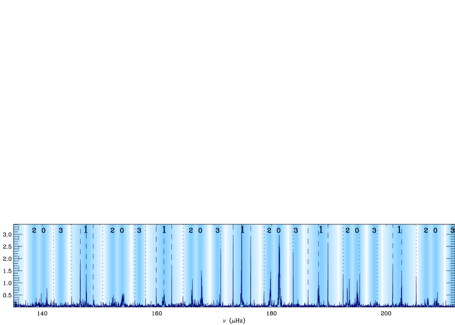
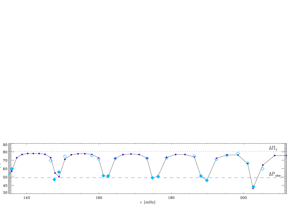
Figure 1: Top: Power density spectrum of the star KIC 9882316, with superimposed mode identification provided by the red giant oscillation universal pattern. Dashed (dotted) lines indicates the position of the peaks a priori (a posteriori) identified as $\ell=1$ mixed modes. P-m modes are located close to the positions marked by 1. Bottom: Period spacings $\Delta P=1/\nu_{n_{\mathrm{m}},1}-1/\nu_{n_{\mathrm{m}}+1,1}$ between adjacent mixed modes, as a function of the frequency. The full line and small filled diamonds correspond to the convolution model defined by Eqs. 4 and 5; the g-mode spacing $\Delta\Pi_{1}$ is indicated by the dotted horizontal line; the dashed line indicates the observed spacing, $\Delta P_{\mathrm{obs}}$, which is affected by the mode bumping, measured with the method presented by Mosser et al. (2011a). The large diamonds show the spacing between two observed consecutive modes; full symbols, near the dashed line, correspond to the measurements derived from the modes a priori identified as $\ell=1$ mixed modes; open symbols, just below the dotted line, are obtained from the peaks identified a posteriori as mixed modes.

In Sect. 2, we briefly present the Kepler observations used in this work and explain how g-m modes are identified. Two ways to model the g-m mode pattern are proposed in Sect. 3. Firstly, a simple adhoc model allows us to identify and fit the mixed-mode pattern, and then to relate the mode bumping to the pure p and g mode patterns in red giants. Secondly, we adopt a more physical approach based on the asymptotic formalism for mixed modes developed by Shibahashi (1979) and Unno et al. (1989), and specifically adapted to subgiants and red giants by Goupil et al. (in prep.).

The quality of the asymptotic fit to the data is investigated in Sect. 4. Inferences of this work are presented in Sect. 5, where we show that g-m modes probe simultaneously the physical conditions in the stellar core and the interface between the core and the envelope, where hydrogen burns in a shell.

2 Observations

2.1 Data

The data used are mainly Kepler long-cadence data that have been described in previous papers (e.g. Jenkins et al. 2010; Bedding et al. 2010; Kallinger et al. 2010; Huber et al. 2010; Mathur et al. 2011b; Mosser et al. 2012, and references therein). Original light curves were processed and corrected according to the procedure of García et al. (2011). We analyzed the stars with the highest signal-to-noise ratio spectra obtained from 690-day time series up to the Kepler quarter Q8. The frequency resolution of 16.8 nHz allowed us to measure the global seismic parameters $\Delta\nu$ (large separation between consecutive radial orders) and $\nu_{\mathrm{max}}$ (central frequency of the oscillation power excess) in 1180 targets using the envelope autocorrelation method (Mosser & Appourchaux 2009). Results provided by this method agree closely with other methods, as shown by Hekker et al. (2011).

The evolutionary status of the red giants was determined for 640 stars from $\Delta P_{\mathrm{obs}}$, measured using the automated method developed by Mosser et al. (2011a). This method requires the precise determination of the expected location of the theoretical $\ell=1$ pure p modes. As the power-of-power method described by Bedding et al. (2011), it is mostly sensitive to the bumped spacing $\Delta P_{\mathrm{obs}}$ and is therefore only a lower limit for the true g-mode spacing $\Delta\Pi_{1}$.

Since we deal in this work with period spacing measurements, it is convenient to translate the frequency resolution into period resolution. At 20, 40, 80, and 160 $\mu$Hz, this corresponds to about 49, 12, 3, and 0.8 s, respectively. This rapid variation (as $\nu^{-2}$) shows that our ability to measure period spacings declines strongly at low frequency.

The oscillation spectra of long-cadence data have a Nyquist frequency of 283.5 $\mu$Hz. To include stars from the lower part of the RGB in our analysis, we must turn to the Kepler short-cadence data (58.8 s instead of 29.4 min), whose Nyquist frequency is much higher. However, since we are only interested in the red giants and not in subgiants or main-sequence stars, we must add an upper limit to the frequency range that we use. It is easy to exclude the main-sequence stars because they are at much higher frequencies than we consider and do not show mixed modes. Excluding the subgiants is more problematic. To guide us in these choices we searched published analyses of individual CoRoT and Kepler giants and subgiants (see di Mauro et al. 2011; Jiang et al. 2011; Deheuvels et al. 2010; Mathur et al. 2011a; Campante et al. 2011). Based on these results, we derived an upper limit on the large separation of $\Delta\nu=40\,\mu$Hz. Note that this is a conservative limit; we neither claim that all red giants have $\Delta\nu\leq 40\,\mu$Hz, nor that all stars with $\Delta\nu\leq 40\,\mu$Hz are red giants. From the analysis of the red giant radii (Verner et al. 2011) and of the near-surface offsets (White et al. 2011a), we verified that the limit value at $40\,\mu$Hz is adequate for our work.

Our sample includes the two red giants with long-duration data sets from the publications listed above, plus a selection from the one-month short-cadence data survey data (Chaplin et al. 2010). These comprise 15 stars with high signal-to-noise oscillation spectra and $\Delta\nu$ in the range [20, 40 $\mu$Hz], to complement the long-cadence data. The signal-to-noise ratio is defined from the envelope autocorrelation function (Mosser & Appourchaux 2009). In making the selection, we were also mindful of the need to include stars with a wide range of masses, the mass being estimated from the asteroseismic scaling relation, as in Mosser et al. (2010), and using the effective temperature given in the Kepler Input Catalog (Brown et al. 2011).

As shown below in Fig. 3, the selected short-cadence stars in the less evolved region of the RGB show properties that extend and are consistent with the analysis primarily based on long-cadence data.

2.2 Detection of $\ell=1$ g-m modes

Red giant oscillation observations have revealed many extra modes that are not explained by the p-mode asymptotic pattern (Bedding et al. 2010; Mosser et al. 2010). These modes have been identified as $\ell=1$ mixed modes (Beck et al. 2011). However, further work showed that some giants, although not all, show very many mixed modes. A careful examination of a few cases has revealed that these modes are present everywhere in the spectrum, not just close to the expected location of the pure p modes. A representative example is shown in Fig. 1. Dozens of similar cases have been found, and 218 of them are considered in this paper.

A multi-stage process was used to identify the $\ell=1$ g-m modes that lie far from the theoretical location of pure p modes. First, the determination of the background (Mathur et al. 2011b; Mosser et al. 2012) allowed us to identify peaks that can be reliably attributed to oscillations. Then, we used the so-called universal pattern to locate the short-lived radial and non-radial pressure modes very precisely (Mosser et al. 2011b). The universal pattern provides a global description of the red giant oscillation pattern. Comparison with a local description is given by Kallinger et al. (2011).

According to Dupret et al. (2009), mixed modes should have noticeable amplitudes only close to the location of the pure p modes. However, there is evidence from the data that mixed modes are observed throughout the spectrum. Given the relative positions of the g- and p-mode cavities for modes of different degree, the $\ell=1$ mixed modes are most likely to be visible, which is what we assume here. Therefore, unassigned peaks in the spectrum were considered as candidates for being dipole g-m modes and were used to construct a period-spacing diagram (Fig. 1). The threshold level used for excluding peaks caused by noise was set empirically at eight times the background value, such that the probability of including a spurious noise peak was less than 1/100. If rotational splitting was present (Beck et al. 2012) we kept only the central $m=0$ component.

By focusing on red giant spectra with very many g-m modes (Fig. 1), we can address the full identification of the $\ell=1$ mixed-mode pattern. The measurement of $\Delta\Pi_{1}$, rather than only $\Delta P_{\mathrm{obs}}$, requires a dedicated modeling as presented below.

3 Parameterization of mixed modes

Mixed modes result from the coupling of p and g waves. We have adopted the description of the universal oscillation pattern of red giants for the p modes (Mosser et al. 2011b). The pure p-mode eigenfrequency pattern can then be expressed as

$$\nu_{n_{\mathrm{p}},\ell}=\left(n_{\mathrm{p}}+{\ell\over 2}+\varepsilon(\Delta\nu)-d_{0\ell}(\Delta\nu)+{\alpha\over 2}[n_{\mathrm{p}}-n_{\mathrm{max}}]^{2}\right)\Delta\nu,$$ (1)

where $\Delta\nu$ is the large separation, $n_{\mathrm{p}}$ is the p-mode radial order, $\ell$ is the angular degree, $\varepsilon$ is the phase offset (which is a function of $\Delta\nu$), $d_{0\ell}$ accounts for the so-called small separation, and $n_{\mathrm{max}}=\nu_{\mathrm{max}}/\Delta\nu$. The constant $\alpha$ represents the mean curvature of the p-mode oscillation pattern and has a value of about 0.008, which is derived from the detailed analysis of the radial-oscillation pattern with the method presented by Mosser (2010).

We next consider the asymptotic development of pure gravity dipole modes derived by Tassoul (1980). To first order, the periods follow

$$P_{n_{\mathrm{g}},\ell=1}=(|n_{\mathrm{g}}|+\alpha_{1})\;\Delta\Pi_{1}\ ,$$ (2)

where $n_{\mathrm{g}}$ is the gravity radial order, $\alpha_{1}$ is a constant, and $\Delta\Pi_{1}$ is the period spacing of dipole g modes. Conventionally, the radial order $n_{\mathrm{g}}$ is defined as a negative integer, in contrast to the positive $n_{\mathrm{p}}$ order, so that the g-mode eigenfrequencies are increasing with increasing order. In the asymptotic limit (e.g. Dziembowski 1977), the period $\Delta\Pi_{1}$ is related to the Brunt-Väisälä frequency $N_{\mathrm{BV}}$ according to

$$\Delta\Pi_{1}={2\pi^{2}\over\sqrt{2}}\ \left[\int_{\mathrm{core}}\!\!{{N_{\mathrm{BV}}\over r}\;\mathrm{d}r}\right]^{-1}.$$ (3)

Measuring $\Delta\Pi_{1}$ gives access to an integral of the Brunt-Väisälä frequency weighted by the inverse of the radius. In red giants, the high density reached in the core gives a high value of $N_{\mathrm{BV}}$. The increase of the core density expected when the star evolves on the RGB results in a decrease of the gravity spacing. When helium ignition occurs in the core, the energy release gives rise to a convective region where $N_{\mathrm{BV}}$ vanishes. This should translate into an increase of $\Delta\Pi_{1}$ (Christensen-Dalsgaard 2011). Hence, we can directly probe the stellar core through the measurement of the Brunt-Väisälä frequency.

3.1 Fitting procedure: an empirical approach

To estimate $\Delta\Pi_{1}$, we first developed an empirical approach for modeling the mode bumping. Deheuvels & Michel (2010) carried out an elegant analysis based on coupled oscillators. Here, we adopt an alternative approach relying on asymptotic relations. In the absence of coupling, the eigenfrequency pattern would simply be the combination of the p- and g-mode asymptotic patterns. We denote this pattern by $\hat{\nu}(k)$, restricted to dipole modes, with the index $k$ enumerating the eigenfrequencies. In the $\Delta\nu$-wide interval centered on $\nu_{\mathrm{max}}$, according to Eqs. 1 and 2 we have one dipole p mode and $\mathcal{N}\simeq\Delta\nu\,\Delta\Pi_{1}^{-1}\nu_{\mathrm{max}}^{-2}$ g modes.

To enumerate the mixed modes, we need to introduce a mixed-mode index. We define it as $n_{\mathrm{m}}=n_{\mathrm{g}}+n_{\mathrm{p}}$, with $n_{\mathrm{g}}$ and $n_{\mathrm{p}}$ being the gravity and pressure radial orders. This definition, with negative values of $n_{\mathrm{g}}$, hence of $n_{\mathrm{m}}$, provides an accurate and continuous numbering of the mixed modes. However, it is not equal to the mixed-mode radial order, which indicates the number of radial nodes in the wavefunction and is given by $|n_{\mathrm{g}}|+n_{\mathrm{p}}$.

A non-negligible coupling is observed (Fig. 1), so that we have no direct access to the uncoupled p and g eigenfrequencies $\hat{\nu}$. We found that the mixed-mode pattern can be reproduced by a redistribution of the p and g eigenfrequencies according to the convolution of the unperturbed p-g pattern with a coupling function $\mathcal{F}$. This convolution model, which is easy to implement numerically, reproduces the effect of the coupling: it simply redistributes the eigenfrequency differences, with the signature of the theoretical pure p modes expressed by the mode bumping. Instead of having $\mathcal{N}$ gravity modes at $\nu_{\mathrm{max}}$ in a $\Delta\nu$-wide interval, there are $\mathcal{N}+1$ mixed modes, with modes bumped in the p-m mode region centered on the theoretical position of the uncoupled p mode. In practice, the eigenfrequency differences of the uncoupled pattern are redistributed according to

$$\nu(n_{\mathrm{m}})-\nu(n_{\mathrm{m}}-1)=\sum_{k=n_{\mathrm{m}}-\mathcal{N}}^{n_{\mathrm{m}}+\mathcal{N}}\bigl{(}\hat{\nu}(k)-\hat{\nu}(k-1)\bigr{)}\ \mathcal{F}_{n_{\mathrm{m}}}(\hat{\nu}(k)).$$ (4)

For clarity, we used $\nu(n_{\mathrm{m}})\equiv\nu_{n_{\mathrm{m}},\ell=1}$. We tested different coupling functions and found the best fit with a Lorentzian:

$$\mathcal{F}_{n_{\mathrm{m}}}(\hat{\nu})={1\over 1+\displaystyle{\left({\hat{\nu}-\hat{\nu}(n_{\mathrm{m}})\over C\Delta\nu}\right)^{2}}}\ ,$$ (5)

with the coupling factor $C$ , of about 0.2. In Sect. 3.2, we justify the use of this empirical function. Importantly, the fit of the g-m mode pattern allows us to determine $\Delta\Pi_{1}$.

Figure 1 (bottom) shows the period differences $\Delta P=1/\nu_{n_{\mathrm{m}},1}-1/\nu_{n_{\mathrm{m}}+1,1}$ between adjacent mixed modes as a function of their frequency. All observed period spacings are smaller than the asymptotic g-mode spacing $\Delta\Pi_{1}$. The fit to all observed mixed modes with the convolved frequencies allows us to identify almost all significant peaks in the power density spectrum. It then provides a measure of the gravity period $\Delta\Pi_{1}$, whereas the fit to the p-m modes is only able to give $\Delta P_{\mathrm{obs}}$. While Stello (2011) found that two parameters were needed to fit the width and depth of the bumping of large series of stellar models, we note that a single parameter $C$ is enough for modeling the mode bumping in the stars presented here, since the width and the depth of the bumping are correlated. This is because the mode bumping has to relate the coupling of one p mode per $\Delta\nu$-wide frequency range: a low depth implies a large width, and vice versa.

Finally, the agreement between the observations and the model allows us to enlarge the set of peaks identified as g-m modes in Sect. 2.2. Peaks with a height five times the background can be assigned to the g-m mode pattern when there is close agreement with the model.

The convolution model provides a very precise but only empirical fit. Therefore, we have also developed a more physical approach.

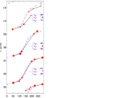
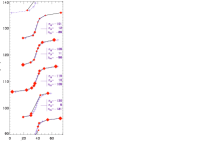
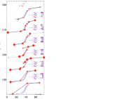
Figure 2: Period échelle diagrams of five representative stars, two in the clump (two left-most panels) and three on the RGB, sorted by increasing $\Delta\nu$. The x-axis shows the period modulo of the gravity spacing $\Delta\Pi_{1}$; the y-axis is the frequency. Diamonds indicate the observed modes, with a size proportional to the mode height. Dashed lines and crosses correspond to the asymptotic fit. Pressure and gravity orders ($n_{\mathrm{p}}$, $n_{\mathrm{g}}$, respectively) and mixed-mode index $n_{\mathrm{m}}$ are given for the mixed modes located near the pressure radial modes. The most p mode-like part of the pattern is located in the middle of the range, at $1/\nu=\Delta\Pi_{1}/2\ (\hbox{modulo }\Delta\Pi_{1})$.

3.2 Asymptotic development

Shibahashi (1979) and Unno et al. (1989) provided an asymptotic relation for p-g mixed modes. In this framework, eigenfrequencies are derived from an implicit equation relating the coupling of the p and g waves (Unno et al. 1989, their Eq. 16.50):

$$\tan\theta_{\mathrm{p}}=q\ \tan\theta_{\mathrm{g}},$$ (6)

where $\theta_{\mathrm{p}}$ and $\theta_{\mathrm{g}}$ are the p- and g-wave phases. The dimensionless coefficient $q$ measures the level of mixture of the p and g phases: $q=0$ is equivalent to no coupling, and maximum coupling occurs for $q=1$. According to the first-order development in Unno et al. (1989), $q$ is supposed to be in the range [0, 1/4]. A similar expression was found by Brassard et al. (1992), but for the coupling of g waves trapped in two different Brunt-Väisälä cavities of ZZ Ceti stars.

Equation 6 supposes that the asymptotic mixed-mode relation closely follows the asymptotic relations of p and g modes (Eqs. 1 and 2). Owing to the complexity of the coupling, the asymptotic relation has no explicit expression. However, following Unno et al. (1989), we consider the p and g phases of Eq. 6:

$$\theta_{\mathrm{p}} = \pi{\nu\over\Delta\nu},$$ (7)

$$\theta_{\mathrm{g}} = \pi{1\over\nu\Delta\Pi_{1}}.$$ (8)

We then introduce the uncoupled solutions of the p modes in Eq. 6 and express it for the dipole mixed modes coupled to the pure p mode $\nu_{n_{\mathrm{p}},\ell=1}$ (Eq. 1) as

$$\nu=\nu_{n_{\mathrm{p}},\ell=1}+{\Delta\nu\over\pi}\arctan\left[q\tan\pi\left({1\over\Delta\Pi_{1}\nu}-\varepsilon_{\mathrm{g}}\right)\right].$$ (9)

In practice, we assume that all dipole modes in the range $[\nu_{n_{\mathrm{p}},\ell=1}-\Delta\nu/2\ ;\ \nu_{n_{\mathrm{p}},\ell=1}+\Delta\nu/2]$ are coupled with $\nu_{n_{\mathrm{p}},\ell=1}$. The constant $\varepsilon_{\mathrm{g}}$ in Eq. 9, already present in Brassard et al. (1992) for the coupling of g waves in two distinct cavities, derived from Goupil et al. (in prep.) for the coupling of p and waves, ensures that we obtain g-m mode periods close to $(n_{\mathrm{g}}+1/2+\varepsilon_{\mathrm{g}})\;\Delta\Pi_{1}$, as expected when the coupling is weak.

For each pressure radial order $n_{\mathrm{p}}$, one derives from Eq. 9 $\mathcal{N}+1$ solutions, with $\mathcal{N}\simeq\Delta\nu\,\Delta\Pi_{1}^{-1}\nu_{\mathrm{max}}^{-2}$ as defined previously. The value of $\Delta\Pi_{1}$ is then derived from a least-squares fit of the observed values, defined as in Sect. 2.2, to the asymptotic solution. Initially, the coupling factor was fixed to be its mean value $\langle q\rangle$, which depends on the evolutionary status. Once $\Delta\Pi_{1}$ was determined, the value of the coupling factor was then iterated, with $\Delta\Pi_{1}$ being fixed. A stable solution for $\Delta\Pi_{1}$ and $q$ was found after only a few iterations.

The qualitative agreement of the fit to the mixed-mode asymptotic relation can be shown in period échelle diagrams (Fig. 2). In the classical échelle diagram, a convenient plot of the p-mode pattern, the x-axis is defined as the frequency modulo of the large separation $\Delta\nu$. Here, to represent mixed modes with periods close the g-mode period pattern, the x-axis of the period échelle diagram is defined as the period modulo $\Delta\Pi_{1}$ (Bedding et al. 2011). This representation is also used for g modes in dense stars (e.g. Pablo et al. 2011). The absolute position of the pattern in the period échelle diagram depends on the unknown term $\varepsilon_{\mathrm{g}}$, which is supposed to be small. We note that the best fits gives $1/2+\varepsilon_{\mathrm{g}}\neq 0\ (\hbox{modulo }1)$. Since the fits do not indicate any trend in $\varepsilon_{\mathrm{g}}$, and since its determination can only be made in modulo 1, we have chosen to fix its value. For simplicity, we considered $\varepsilon_{\mathrm{g}}=0$, as implicitly assumed by Bedding et al. (2011). The S-shape observed in the period échelle diagram, with one S-pattern per $\Delta\nu$-wide interval, is the signature of a coupling with a coupling coefficient close to $\langle q\rangle$. A lower coupling coefficient would correspond to steeper central segments, whereas stronger coupling would correspond to more inclined segments.

The asymptotic solutions were compared with those of the empirical convolution model and they cannot be distinguished. This close agreement follows from the fact that the Lorentzian form introduced in Eq. 5 is the derivative of the $\arctan$ function, which appears in the asymptotic expression for the coupling. Strictly speaking, our solutions are only quasi-asymptotic, since we use in Eq. 9 the pressure mode pattern described by Eq. 1, which is not purely asymptotic. However, for simplicity, we refer to it as asymptotic. We also note that any a priori dipole pure p-mode pattern, such as that derived from a precise fit to the radial modes, can be used for the p-mode frequencies $\nu_{n_{\mathrm{p}},\ell=1}$ in Eq. 9.

In the next sections, we examine the results from the fitting to the observed mixed-mode pattern with the asymptotic relation, and we use it to derive important information on the red giant oscillation spectra.

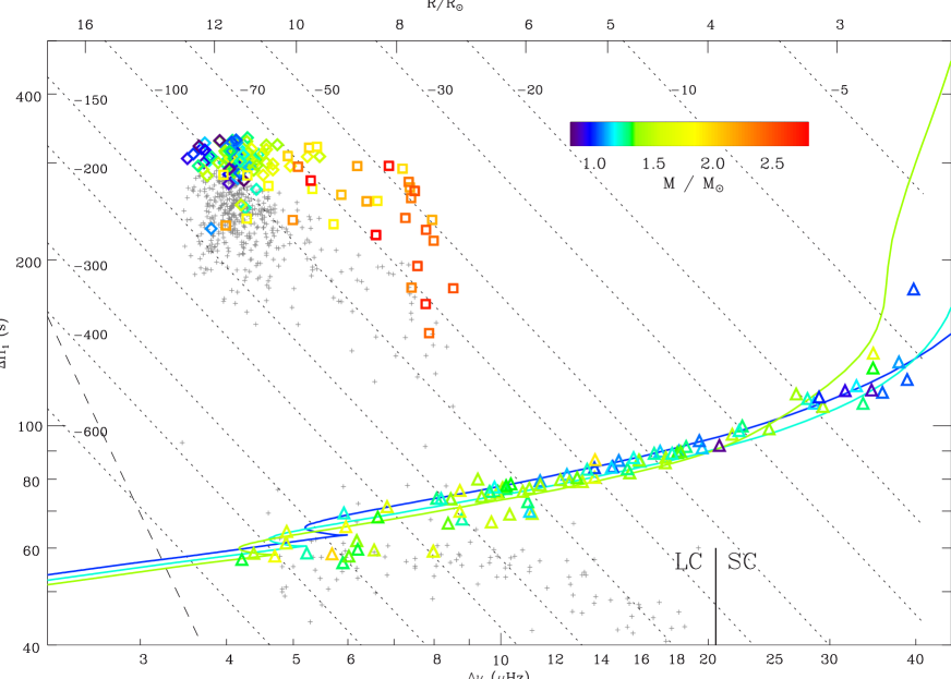
Figure 3: Gravity-mode period spacing $\Delta\Pi_{1}$ as a function of the pressure-mode large frequency spacing $\Delta\nu$. Long-cadence data (LC) have $\Delta\nu\leq 20.4\,\mu$Hz. RGB stars are indicated by triangles; clump stars by diamonds; secondary clump stars by squares. Uncertainties in both parameters are smaller than the symbol size. The seismic estimate of the mass is given by the color code. Small gray crosses indicate the bumped periods $\Delta P_{\mathrm{obs}}$ measured by Mosser et al. (2011a). Dotted lines are $n_{\mathrm{g}}$ isolines. The dashed line in the lower left corner indicates the formal frequency resolution limit. The upper x-axis gives an estimate of the stellar radius for a star whose $\nu_{\mathrm{max}}$ is related to $\Delta\nu$ according to the mean scaling relation $\nu_{\mathrm{max}}=(\Delta\nu/0.28)^{1.33}$ (both frequencies in $\mu$Hz). The solid colored lines correspond to a grid of stellar models with masses of 1, 1.2 and $1.4\,M_{\odot}$, from the ZAMS to the tip of the RGB.

4 Mixed modes and mode bumping

4.1 Gravity spacings

Thanks to the g-m modes, the fit to the mixed-mode pattern provides us with the measurement of the gravity spacing $\Delta\Pi_{1}$. The number of stars with sufficient g-m modes is limited to 218 red giants. Measuring $\Delta\Pi_{1}$ precisely helps us to improve the criteria for distinguishing the evolutionary status of the stars, namely that RGB and clump stars clearly show different distributions, as already observed for the bumped spacings (Bedding et al. 2011; Mosser et al. 2011a). A $\Delta\nu$ – $\Delta P_{\mathrm{obs}}$ diagram is very useful for distinguishing the evolutionary status of the stars. We plotted our current results using such a diagram, but with $\Delta\Pi_{1}$ instead of $\Delta P_{\mathrm{obs}}$ (Fig. 3). This diagram allows us to emphasize the difference between RGB giants, which are burning hydrogen in a shell around the helium core and ascend the RGB, and clump stars, which have convection in the helium-burning core (e.g. Kippenhahn & Weigert 1990, chap. 32). Christensen-Dalsgaard (2011) has explained the higher values of $\Delta\Pi_{1}$ in red-clump stars by the fact that g modes are excluded from this convective core. Table 1 summarizes the properties of the stars presented in this paper.

Stars with different evolutionary states are clearly located in different regions of the $\Delta\nu$ – $\Delta\Pi_{1}$ diagram (Fig. 3). Compared to the bumped spacings, the gravity spacings show a lower dispersion, especially for the red-clump stars. If we set the mass limit between the first and the secondary clump at 1.8 $M_{\odot}$, the mean value of $\Delta\Pi_{1}$ in the clump is $297\pm 23$ s. The secondary clump stars show a broader distribution, with values in the range [150, 300 s]. For RGB stars, $\Delta\Pi_{1}$, in the range [60, 120 s], has a clear relationship with $\Delta\nu$. We note a slight decrease of $\Delta\Pi_{1}$ during the ascent of the first part of the RGB (for $\Delta\nu$ decreasing down from 40 to 7 $\mu$Hz, equivalent to a radius increase from about 2.5 to about 8 $R_{\odot}$). This evolution corresponds to the contraction of the core when the star ascends the RGB. The tight $\Delta\nu$ – $\Delta\Pi_{1}$ relation indicates that the expansion of the envelope is closely related to the contraction of the core.

We compared the observed $\Delta\nu$ – $\Delta\Pi_{1}$ relation with the same quantities obtained from a grid of stellar models with masses of 1, 1.2, and $1.4\,M_{\odot}$, from the zero age main sequence (ZAMS) to the tip of the RGB. This range of mass corresponds to the observed masses derived from the seismic estimates. These models were obtained using the stellar evolution code CESAM2k (Morel & Lebreton 2008), assuming a gray Eddington approximation and the Böhm-Vitense mixing-length formalism for convection with a mixing-length parameter $\alpha=1.6$. The initial chemical composition follows Asplund et al. (2005), with a helium mass fraction of $0.2485$. The period spacing was computing using Eq. 3, while the large separation was computed using the asymptotic description $\Delta\nu=(2\int_{0}^{R}\mathrm{d}r/c)^{-1}$, where $c$ is the sound speed.

Qualitatively similar evolution was already shown in modeling results (Bedding et al. 2011; White et al. 2011b; Christensen-Dalsgaard 2011), but without a direct comparison to $\Delta\Pi_{1}$. In Fig. 3, we note a close agreement between observed and modeled values for $\Delta\nu\geq 11\,\mu$Hz. The spread around the evolution tracks is low, less than 2 %. However, we do not see in the observed data the clear mass dependence present in the models. The larger spread in $\Delta\Pi_{1}$ for RGB stars with $\Delta\nu$ less than 11 $\mu$Hz is unexplained and deserves more work. Various reasons have to be investigated, such as stellar rotation, the influence of the mixing length and of overshooting, or an inadequacy of the asymptotic relation in some specific cases. It may also correspond to the first dredge-up (Christensen-Dalsgaard 2011), which seems to appear too late in the evolution models.

Finally, we note the presence of five red giants with a large separation around 4.2 $\mu$Hz and a g-mode spacing around 250 s, in a region of the $\Delta\nu$ – $\Delta\Pi_{1}$ diagram clearly distinct from the red clump. These apparent outliers are most plausibly red giants that have exhausted helium in their core and have begun the ascent of the asymptotic giant branch.

The frequency resolution is not high enough to provide reliable measurements of $\Delta\Pi_{1}$ in RGB stars with $\Delta\nu\leq 4\,\mu$Hz.

4.2 Agreement with the asymptotic description

We have found that all oscillation patterns with very many g-m modes can be fitted with the asymptotic relation. The highest precision is obtained in spectra showing the most g-m modes. G-m modes present and identified near the $\ell=0$ and 2 ridges allow the most precise observations. On the other hand, the absence of g-m modes most often hampers the measurement of $\Delta\Pi_{1}$, or results in a limited accuracy, due to the possible misidentification of the period spacing. The number of accurate determinations of $\Delta\Pi_{1}$ is therefore limited by the number of stars with very many g-m modes (218 stars studied in this work).

A limited number of discrepant cases may occur. All these correspond to oscillation spectra with relatively few peaks extracted with the criterion defined in Sect. 2.2, and never to a clear disagreement with the asymptotic form. They fall mainly into two categories:
- Because dipole g-m modes are observed everywhere in the spectrum, possible errors may occur when they are located close to other modes and may be mis-identified. The $\ell=2$ and $\ell=3$ non-radial modes may also present complex mixed-mode patterns, so that an unambiguous identification of the mixed modes is not possible. This occurs mostly at low frequency, when the resolution limit is a problem. The increase of the observation time as the Kepler mission continues will solve these problems.
- In some cases, a gradient or a modulation of $\Delta\Pi_{1}$ possibly explains the observations. These specific cases deserve additional studies. Observationally, high signal-to-noise ratio spectra are required for the analysis of small-amplitude mixed modes in a very large frequency range. We show an example where a variation in $\Delta\Pi_{1}$ of about 2.5 % is necessary to fit the lower and upper part of the spectrum (Fig. 5). According to the propagation diagram, high-frequency g waves probe a less extended cavity than low-frequency waves. This explains the higher value of $\Delta\Pi_{1}$ measured at high frequency. Theoretically, the link of this phenomenon with the shell structure of the red giant interior has to be investigated in more detail.

Finally, a few remaining peaks not identified as dipole mixed modes are likely to be $\ell=2$ or 3 mixed modes. Their study will require additional work.

4.3 Advantages of the asymptotic method

The derived values of $\Delta\Pi_{1}$ can be compared to the values $\Delta P_{\mathrm{obs}}$ (Fig. 6). The ratio $\Delta P_{\mathrm{obs}}/\Delta\Pi_{1}$ depends on the number of g-m modes effectively used for deducing $\Delta P_{\mathrm{obs}}$. A low ratio may occur because only few mixed modes close to the p-m modes are detected, or because the coupling is weak. Then, deriving $\Delta\Pi_{1}$ from $\Delta P_{\mathrm{obs}}$ is possible but not precise. We also note that rotational splittings (Sect. 5.2) mimic low $\Delta P_{\mathrm{obs}}$ values, especially for RGB stars with large $\Delta\nu$.

The measurement of the period spacing is correlated with the measurement of $\varepsilon_{\mathrm{g}}$. At this stage, we have only determined pairs of values ($\Delta\Pi_{1}$, $\varepsilon_{\mathrm{g}}$). The uncertainties in $\Delta\Pi_{1}$ calculated with $\varepsilon_{\mathrm{g}}=0.5$ are very small, typically about 0.2 s for clump stars and 0.02 s for RGB stars (Table 1). Full uncertainties in $\Delta\Pi_{1}$ have to take into account the unknown value of $\varepsilon_{\mathrm{g}}$. They can be estimated for the stars with the most g-m modes. The uncertainties vary inversely with the number of gravity nodes in the core: in relative value, they are typically better than $1/(2\nu_{\mathrm{max}}\Delta\Pi_{1})$. This represents about 0.5 to 1 % for clump stars, and between 0.3 and 1 % for RGB stars. We note that this high accuracy of the measurement of $\Delta\Pi_{1}$ is based on the close agreement with the asymptotic development. As shown by Mosser et al. (2011a), the high absolute values of the gravity order $n_{\mathrm{g}}$ ensure the validity of the asymptotic relation and therefore strongly support a close agreement. The coupling $q$ is also derived, with a lower precision. Again, the uncertainties are much reduced when g-m modes far from the p-m modes are observed.

The method is not only precise; it proves to be efficient, too. For instance, Bedding et al. (2011) were able to identify the g-mode spacing $\Delta\Pi_{1}$ in the star KIC 6928997 thanks to the measurement of 21 mixed modes, with a Fourier spectrum performed from a 13-month-long time series. We can now identify 45 mixed modes, thanks to the longer observation run (22 months) and the fit to the asymptotic relation (Fig. 2).

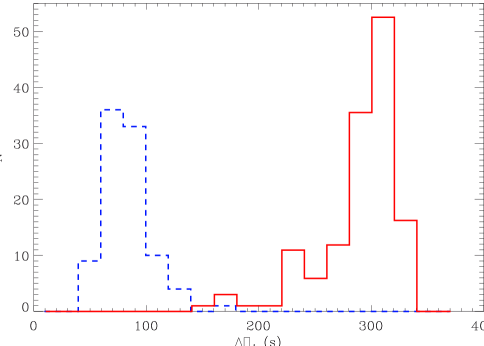
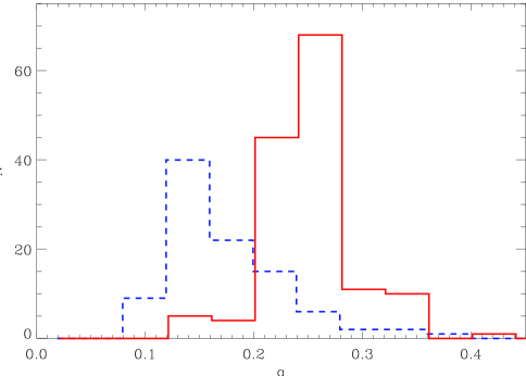
Figure 4: Top: histogram of $\Delta\Pi_{1}$, showing RGB stars (dashed line) and clump stars (solid line). Bottom: histogram of $q$.

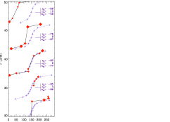
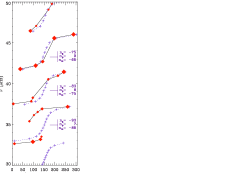
Figure 5: Period échelle diagrams of the star KIC 9332840 based on two different values of $\Delta\Pi_{1}$, presented as in Fig. 2. Left: the fit at low frequency requires $\Delta\Pi_{1}=298.9\pm 0.2$ s. Right: the high-frequency pattern is better reproduced with $\Delta\Pi_{1}=306.3\pm 0.2$ s.

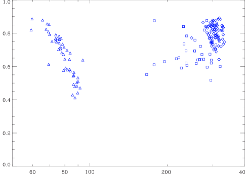
Figure 6: Ratio $\Delta P_{\mathrm{obs}}/\Delta\Pi_{1}$ as a function of the period spacing $\Delta\Pi_{1}$. Symbols have the same definition as in Fig. 3.

Table 1: Characteristic parameters of the red giants named in the paper

KIC number	$\Delta\nu$	$\nu_{\mathrm{max}}^{(a)}$	$\Delta\Pi_{1}^{(b)}$	$q$	$R_{\mathrm{seis}}^{(c)}$	$M_{\mathrm{seis}}^{(c)}$	evolutionary
	($\mu$Hz)	($\mu$Hz)	(s)		($R_{\odot}$)	($M_{\odot}$)	status(d)
2013502	5.72	61.2	232.20$\pm$0.10	0.27$\pm$0.03	10.12	1.87	2nd clump
3744043	9.90	110.9	75.98$\pm$0.10	0.16$\pm$0.03	6.24	1.32	RGB
4044238	4.07	33.7	296.35$\pm$0.15	0.32$\pm$0.05			clump
5000307	4.74	42.2	323.70$\pm$0.30	0.26$\pm$0.06	10.36	1.38	clump
6928997	10.06	120.0	77.21$\pm$0.02	0.14$\pm$0.04	6.36	1.44	RGB
8378462	7.27	90.3	238.30$\pm$0.20	0.23$\pm$0.05	9.39	2.42	2nd clump
9332840	4.39	41.4	298.9$\pm$0.2 - 306.3$\pm$0.2	0.20$\pm$0.05	11.67	1.69	clump
9882316	13.68	179.3	80.58$\pm$0.02	0.15$\pm$0.05	5.41	1.63	RGB

Asymptotic mixed-mode parameters of the red giant oscillation spectra shown in the paper.

^(a): $\nu_{\mathrm{max}}$ indicates the central frequency of the oscillation power excess.
^(b): this uncertainty assumes that $\varepsilon_{\mathrm{g}}$ is fixed to 1/2.
^(c): $M_{\mathrm{seis}}$ and $R_{\mathrm{seis}}$ are the asteroseismic estimates of the stellar mass and radius from scaling relations, using $T_{\mathrm{eff}}$ from the Kepler Input Catalog (Brown et al. 2011) .
^(d): the division between RGB and clump stars is derived from Fig. 3; the limit between the primary and secondary (2nd clump) clump stars is set at 1.8 $M_{\odot}$.
The complete table can be downloaded at the CDS via anonymous ftp to cdsarc.u-strasbg.fr (130.79.128.5) or via http://cdsweb.u-strasbg.fr/cgi-bin/qcat?J/A+A/

5 Discussion

5.1 Overlapping modes

The close agreement with the asymptotic description for those stars with very many mixed modes now allows us to extend the mixed-mode identification to those stars with relatively few mixed modes. Throughout, it is possible to identify the vast majority of the peaks with a height five times above the mean background level. This has also consequences for the degree identification.

Dipole mixed modes can be present in the region of radial modes and $\ell=2$ modes (Fig. 7). The narrow peaks corresponding to very long-lived g-m modes present in the vicinity of the structure created by the short-lived radial p modes or complex $\ell=2$ patterns are $\ell=1$ mixed modes. Coincidences are of course possible. However, there would be so many coincidences that their spurious existence is doubtful. Therefore, we argue that a correct identification of the g-m mode pattern is definitely necessary for addressing specific points such as the precise mode identification or the measurement of the width of the radial modes (Baudin et al. 2011). We also note that the heights of $\ell=1$ g-m modes in the vicinity of $\ell=0$, 2, or 3 modes is sometimes significantly boosted. This may result from interference. We cannot exclude the possibility that the g-m mode heights are boosted by the energy of the other degree modes, even if the orthonormality of the spherical harmonics of different degrees seems to rule out mode coupling when oscillation amplitudes are low, as is the case here. This deserves more observations and simulations.

As already noted by Mosser et al. (2012), $\ell=1$ mixed modes are present in the region of $\ell=3$ modes, so that distinguishing true $\ell=3$ modes is difficult. Figure 8 presents a typical case, with $\ell=3$ mixed modes surrounded by $\ell=1$ mixed modes. We note the frequent interferences between $\ell=1$ g-m modes and $\ell=3$, and have to conclude that the ensemble observations reporting the observations of $\ell=3$ modes with high amplitudes may be overinterpreted (Bedding et al. 2010; Huber et al. 2010; Mosser et al. 2012). A significant number of peaks close to the expected location of $\ell=3$ modes are most likely $\ell=1$ g-m modes.

5.2 Rotational splittings and mixed modes

Beck et al. (2012) have recently reported non-rigid rotation in red giants, detected through a rotational splitting that varies with frequency. In many cases, especially for stars with $\Delta\nu$ above 10 $\mu$Hz, the rotational splitting is so close to the mixed-mode spacing that the direct identification of the rotational multiplets is difficult. However, we showed that the use of the asymptotic relation is able to provide the correct identification of the rotational multiplets when coupled to a simple ad-hoc model accounting for non-rigid rotation. We found that an empirical modeling that takes into account the modulation of the rotational splitting with a Lorentzian profile provides an acceptable fit (Fig. 9). This profile $\mathcal{R}$ accounts for both the differential rotation observed by Beck et al. (2012) and the varying Ledoux coefficients (Ledoux 1951). Because the maximum observed rotational splitting $\delta\nu_{\mathrm{rot,g}}$ is small, $\mathcal{R}$ provides a splitting of the form

$$\nu(n_{\mathrm{m}},1,m)=\nu(n_{\mathrm{m}},1)+m\ \mathcal{R}(n_{\mathrm{m}},1)\ \delta\nu_{\mathrm{rot,g}},$$ (10)

with $m$ being the azimuthal order. Locally, around a given dipole pure p mode of radial order $n_{\mathrm{p}}$, for mixed-mode index $n_{\mathrm{m}}$ associated via the coupling to this pressure radial order $n_{\mathrm{p}}$, $\mathcal{R}$ can be expressed as

$$\mathcal{R}_{n_{\mathrm{p}}}(n_{\mathrm{m}},1)=1-{e\over 1+{\displaystyle{\left({\nu(n_{\mathrm{m}},1)-\nu(n_{\mathrm{p}},1)\over\beta\Delta\nu}\right)^{2}}}},$$ (11)

with $\nu(n_{\mathrm{p}},1)$ given by Eq. 1. The constant terms $e$ and $\beta$, empirically determined, are about 0.5 and 0.08, respectively, and $\delta\nu_{\mathrm{rot,g}}$ is the maximum rotational splitting observed for g-m modes. The study of $\delta\nu_{\mathrm{rot,g}}$ was not conducted exhaustively and is beyond the scope of this paper.

Beck et al. (2012) have noted that the heights of the $m=+1$ and $-1$ modes of a given multiplet are very often not symmetric, as observed in the solar case (Chaplin et al. 2001). This emphasizes the interest of the identification of the mixed-mode pattern for a correct identification of the rotational structure of oscillation pattern. Moreover, for similar reasons as those discussed in Sect. 5.1 concerning overlapping modes, we stress that in many cases the prior identification of the mixed-mode pattern is essential to avoid misidentifications. In cases such as presented in Fig. 9, despite a different behavior with frequency of the rotational splittings (almost constant in frequency apart from the periodic modulation due to $\mathcal{R}$) and mixed-mode spacings (varying as $\nu^{-2}$), the near equality between them greatly complicates the identification. For those stars, the observed spacings $\Delta P_{\mathrm{obs}}$ were too small by a factor of about 2, whereas the inferred $\Delta\Pi_{1}$ closely follow the trends observed in Fig. 3.

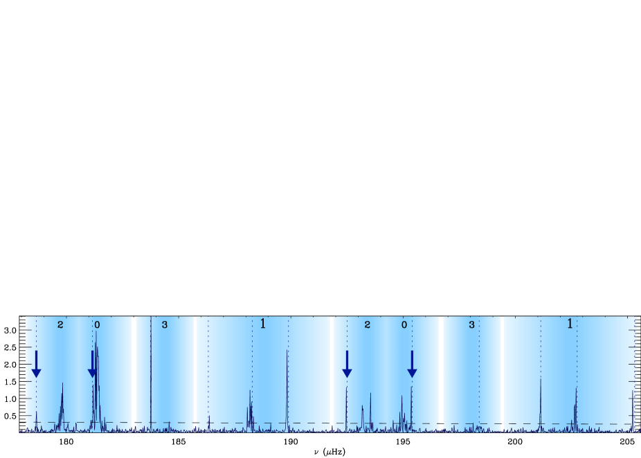
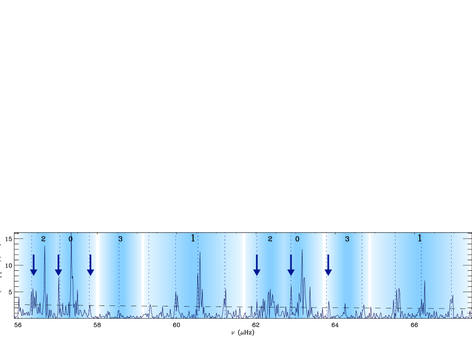
Figure 7: Overlapping mixed modes identified a posteriori in the power density spectra of three red giants. Vertical dotted lines correspond to the dipole mixed-mode frequencies determined using the asymptotic fit. Arrows indicate the modes assigned a posteriori to $\ell=1$ mixed modes. The dashed lines show the threshold level corresponding to eight times the stellar background. Top, KIC 9882316: additional peaks close to the $\ell=2$ and 0 patterns present the characteristics of g-m modes, with a very narrow linewidth. Bottom, KIC 2013502: the peaks at 56.34, 57.06, 57.79, 62.02, 62.88, and 63.77 $\mu$Hz, that is, close to the uninterrupted series of g-m modes, seem to be $\ell=1$ mixed modes. This is not rare.

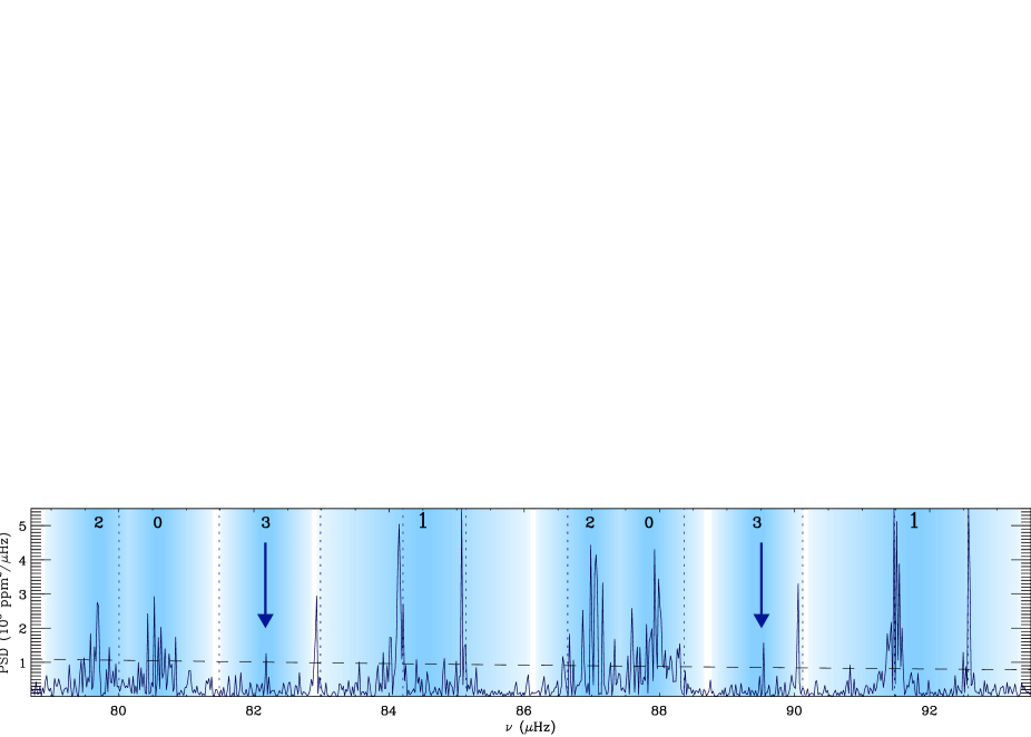
Figure 8: Same as Fig. 7, but with arrows indicating the modes a posteriori assigned to $\ell=3$ mixed modes. The identity of these low-amplitude peaks is certain thanks to the prior identification of $\ell=1$ mixed modes in the vicinity.

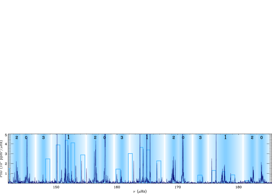
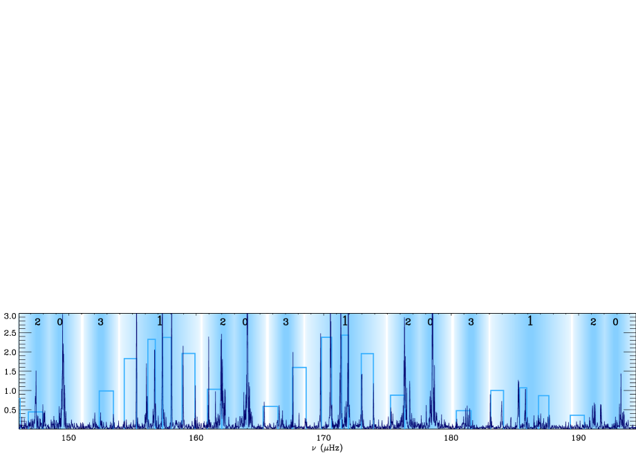
Figure 9: Identification of rotational multiplets in two stars observed with a nearly edge-on inclination and showing nearly equal rotational splittings and mixed-mode spacing. Synthetic $m=\pm 1$ doublets based on the mixed-mode asymptotic relation and on a simple modeling of the differential rotation are close to the observed mixed modes.

5.3 Strength of the coupling

Measuring the factor $q$ precisely is possible for about 75 % of the 218 red giants. We note that the distribution strongly depends on the evolutionary status of the red giants (Fig. 4). The mean values are $q_{\mathrm{RGB}}=0.17\pm 0.03$ and $q_{\mathrm{clump}}=0.25\pm 0.05$. The lower values for RGB stars indicate that the region between the g- and p-mode cavities is larger than for clump stars. We also note the existence of $q$ factors larger than 1/4, contradicting the first-order modeling by Unno et al. (1989). The full interpretation of $q$ in terms of interior structure properties requires more work. Indeed, the exact relation between the factor $q$ and the properties of the region between the g and p cavities remains to be established. The first-order description given by Unno et al. (1989) is clearly not sufficient to explain the values of this coupling constant for red giants. In particular, for $q>1/4$, an extension of the Unno’s description will be necessary.

That $q$ is almost a fixed parameter at fixed evolutionary status has two important consequences. When the quality of the spectra does not allow the identification of g-m modes with tiny amplitudes, deriving a precise value of $\Delta\Pi_{1}$ remains possible, assuming $q=\langle q\rangle$. When only mixed modes close to the p-m modes can be identified, it is still possible to obtain a correct estimate of $\Delta\Pi_{1}$, thanks to a fit restricted to these p-m modes. In that case, the measurement is less precise, but physically more significant than the value $\Delta P_{\mathrm{obs}}$ derived between the p-m modes.

5.4 Mode heights of g-m modes

As previously noted, the observation of numerous g-m modes so far from the expected location of p-m modes is a surprise. Dupret et al. (2009) showed that for high-mass stars (2 to 3 $M_{\odot}$) significant heights are only expected near the p-m modes, in a frequency range limited to about 0.1-0.2 $\Delta\nu$ around them. However, most of the red giants observed by Kepler have a mass much below this range (Table 1). Among them, we have identified spectra with g-m modes observed almost everywhere. However, there are also spectra with only a single p-m mode or a very limited number of mixed modes per pressure radial order, as predicted by Dupret et al. (2009).

Theoretical information on the possible cause of this striking variety is limited at present. Clearly, we may imagine that the coupling conditions between the two cavities may differ significantly between the different red giants. However, we lack a theoretical work similar to Dupret et al. (2009) for low-mass stars in the range 0.8 to 2 $M_{\odot}$. A work like this that would examine the propagation condition would help to interpret the different observations and may give the key for examining the deepest regions of the stars. These regions, at the limit between the p- and g-mode cavities according to the seismic view, correspond to the hydrogen-burning shell. Therefore, the seismic observations allow us to investigate these regions, and to test the different physical conditions, at the red giant bump, before or after the first dredge-up.

We also recall that a population of red giants with very low amplitude dipole modes has been reported by Mosser et al. (2012). Unsurprisingly, the determination of $\Delta\Pi_{1}$ for those stars is not possible. Theoretical work is definitely necessary to understand the different mixed-mode patterns.

5.5 Pure gravity modes?

Our analysis shows that in very many stars with g-m modes, all observed $\ell=1$ modes are mixed modes, with a significant coupling between p and g waves according to the asymptotic formalism. Their frequencies as well as their amplitudes are strongly correlated with the pressure-mode pattern. Mosser et al. (2012) showed that the total visibility of $\ell=1$ mixed modes surrounding a given p mode is consistent with the expected visibility of the corresponding pure p mode, emphasizing the role of the coupling with p modes in observing g modes. This shows that the excitation of mixed modes is closely related to the excitation mechanism of p modes provided by turbulent convection in the uppermost layers of the stellar envelopes.

From the observations, we deduce that we have not detected any pure g modes, whose signature would have been a vertical line in the period échelle diagram. Pure g modes are expected to have very low amplitudes at the stellar surface, which makes them hard to detect. The prevalence of mixed modes is likely to be a consequence of the high density in the red giant core, which ensures that the Brunt-Väisälä frequency is similar to or larger than the p-mode frequencies, thus facilitating wave coupling. It is, of course, difficult to draw many inferences on the core conditions from stars that do not show a large number of g-m modes, except perhaps that the conditions do not favor strong wave coupling which, in itself, may be useful information.

6 Conclusion

The identification of red giant spectra with very many g-m modes and the use of the mixed-mode asymptotic relation proposed by Goupil et al. (in prep.) allowed us to measure the gravity-mode spacing $\Delta\Pi_{1}$. This provides a new and unique way to characterize the physical conditions in the inner radiative regions of the red giant cores.

We have observed in most cases a close agreement between the observed mixed-mode spectra and the asymptotic relation. When this agreement was not met, signal-to-noise ratio considerations were sufficient to explain the disagreement. Complex cases occur when rotational splittings complicate the spectrum. However, a simple modeling of the rotational splitting, accounting for differential rotation, allowed us to separate the rotational splitting from the mixed-mode spacing. The large variation in the height distribution of the g-m modes requires a study similar to that by Dupret et al. (2009), but extended to red giant stars with masses in the range [0.8, 2 $M_{\odot}$].

The identification of the $\ell=1$ g-m modes allows the full identification of all significant peaks in a red giant oscillation spectrum. It also helps to perform the peak bagging more efficiently. We stress that $\ell=1$ g-m modes, present everywhere in the oscillation spectrum, are often overlapping with other degrees. In several cases, the previously reported $\ell=3$ modes are, in fact, $\ell=1$ g-m modes. The identification of the complete $\ell=1$ mixed-mode pattern makes the spectrum clear.

Compared to the seismic constraints provided by the frequencies $\Delta\nu$ and $\nu_{\mathrm{max}}$, which are mainly sensitive to the average stellar structure, the gravity period $\Delta\Pi_{1}$ directly probes the core region. When available, the measurement of the gravity period reaches a high level of accuracy, better than 1 %, thanks to the many gravity nodes observed in the stellar core. A similar accuracy is now necessary in red giant interior models.

We showed that the coupling factor and the heights of g-m modes in red giant oscillation spectra present a large variety of cases. This is due to different physical conditions at the limit between the helium core and the hydrogen envelope in the region where hydrogen burns in shell, where the first dredge-up occurs. Additional work will be carried out to take the full benefit of these new asteroseismic constraints for probing these regions in detail.

We showed that the contraction of the core in stars ascending the RGB occurs with a tight relation between the period spacing and the large separation. Asteroseismic measures provide clear constraints on the red giant structure and evolution.