Coupled Chemistry-Emission Model for Atomic Oxygen Green and Red-doublet Emissions in Comet C/1996 B2 Hyakutake

Abstract

The green (5577 Å) and red-doublet (6300, 6364 Å) lines are prompt emissions of metastable oxygen atoms in the ¹S and ¹D states, respectively, that have been observed in several comets. The value of intensity ratio of green to red-doublet (G/R ratio) of 0.1 has been used as a benchmark to identify the parent molecule of oxygen lines as H₂O. A coupled chemistry-emission model is developed to study the production and loss mechanisms of O(¹S) and O(¹D) atoms and the generation of red and green lines in the coma of C/1996 B2 Hyakutake. The G/R ratio depends not only on photochemistry, but also on the projected area observed for cometary coma, which is a function of the dimension of the slit used and geocentric distance of the comet. Calculations show that the contribution of photodissociation of H₂O to the green (red) line emission is 30 to 70% (60 to 90%), while CO₂ and CO are the next potential sources contributing 25 to 50% ($<$5%). The ratio of the photo-production rate of O(¹S) to O(¹D) would be around 0.03 ($\pm$ 0.01) if H₂O is the main source of oxygen lines, whereas it is $\sim$0.6 if the parent is CO₂. Our calculations suggest that the yield of O(¹S) production in the photodissociation of H₂O cannot be larger than 1%. The model calculated radial brightness profiles of the red and green lines and G/R ratios are in good agreement with the observations made on comet Hyakutake in March 1996.

1 Introduction

The spectroscopic emissions from dissociative products in cometary coma are often used in estimating production rates of respective cometary parent species which are sublimating directly from the nucleus (Feldman et al., 2004; Combi et al., 2004). It is a known fact that at smaller ($<$2 AU) heliocentric distances, the inner cometary coma is dominantly composed of H₂O. The infrared emissions of H₂O molecule are inaccessible from ground because of strong attenuation by the terrestrial atmosphere. Since H₂O does not show any spectroscopic transitions in ultraviolet or visible regions of solar spectrum, one can estimate it’s abundance indirectly based on the emissions from daughter products, like OH, O and H. Thus, tracking emissions of the dissociative products of H₂O has became an important diagnostic tool in estimating the production rate as well as in understanding the spatial distribution of H₂O in comets (Delsemme & Combi, 1976, 1979; Fink & Johnson, 1984; Schultz et al., 1992; Morgenthaler et al., 2001; Furusho et al., 2006). For estimating the density distribution of H₂O from the emissions of daughter species, one has to account for photochemistry and associated emission processes.

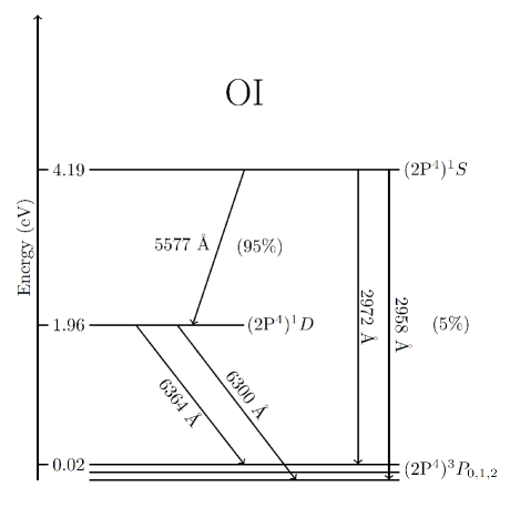
Figure 1: Energy level diagram of atomic oxygen showing different spectroscopic transitions related to ¹S and ¹D states.

The major dissociative channel of H₂O is the formation of H and OH, but a small fraction is also possible in O(³P, ¹S, ¹D) and H₂. The radiative decay of metastable ¹D and ¹S states of atomic oxygen leads to emissions at wavelengths 6300, 6364 Å (red doublet) and 5577 Å (green line), respectively. The energy levels of atomic oxygen and these forbidden transitions are shown in Figure 1. Even though these emissions are accessible from ground-based observatories, most of the times they are contaminated by telluric night sky emissions as well as emissions from other cometary species. Doppler shift of these lines, which is a function of the relative velocity of comet with respect to the Earth, offers a separation from telluric emissions provided a high resolution cometary spectrum is obtained. In most of the cometary observations it is very difficult to separate the green line in optical spectrum because of the contamination from cometary C₂ (1-2) P-branch band emission. The red line 6300 Å emission is also mildly contaminated by the Q-branch emission of NH₂ molecule, but in high resolution spectrum this can be easily resolved.

Since these atomic oxygen emissions result due to electronic transitions which are forbidden by selection rules, solar radiation cannot populate these excited states directly from the ground state via resonance fluorescence. The photodissociative excitation and electron impact excitation of neutral species containing atomic oxygen, and ion-electron dissociative recombination of O-bearing ion species, can produce these metastable states (Bhardwaj & Haider, 2002). If O(¹D) is not quenched by ambient cometary species, then photons at wavelengths 6300 and 6364 Å will be emitted in radiative decay to the ground ³P state. Only about 5% of O(¹S) atoms result in 2972 and 2958 Å emissions via direct radiative transition to the ground ³P state of atomic oxygen. Around 95% of O(¹S) decays to the ground state through O(¹D) by emitting green line (cf. Fig. 1). This implies that if the green line emission is present in cometary coma, the red doublet emission will also be present, but the opposite is not always true. The average lifetime of O(¹D) is relatively small ($\sim$110 s) compared to the lifetime of H₂O molecule ($\sim$8 $\times$ 10⁴ s) at 1 AU. The O(¹S) also has a very short average lifetime of about 0.1 s. Due to the short lifetime of these metastable species, they cannot travel larger distances in cometary coma before de-exciting via radiative transitions. Hence, these emissions have been used as diagnostic tools to estimate the abundance of H₂O in comets (Fink & Johnson, 1984; Magee-Sauer et al., 1990; Morgenthaler et al., 2001). The intensity of O[I] emissions, in Rayleigh, can be calculated using the following equation (Festou & Feldman, 1981)

$$I=10^{-6}\tau_{p}^{-1}\alpha\beta N$$ (1)

where $\tau_{p}$ is the lifetime of excited species in seconds, $\alpha$ is the yield of photodissociation, $\beta$ is the branching ratio, and N is the column density of cometary species in cm^-2.

In the case of red doublet (6300 and 6364 Å), since both emissions arise due to transition from the same excited state (2P^{4 1}D) to the ground triplet state (2P^{4 3}P), the intensity ratio of these two lines should be the same as that of branching ratio of corresponding transitions. Using Einstein transition probabilities, Storey & Zeippen (2000) calculated the intensity ratio of red doublet and suggested that the intensity of 6300 Å  emission would be 3 times stronger than that of 6364 Å  emission, and this has been observed in several comets also (Spinrad, 1982; Fink & Johnson, 1984; Morrison et al., 1997; Cochran & Cochran, 2001; Capria et al., 2005; Furusho et al., 2006; Capria et al., 2008; Cochran, 2008).

The ratio of intensity of green line to the sum of intensities of red doublet can be calculated as

$$\frac{I_{5577}}{I_{6300}+I_{6364}}=\frac{\tau^{-1}_{green}\alpha_{green}N_{green}\beta_{green}}{\tau^{-1}_{red}\alpha_{red}N_{red}(\beta_{6300+6364})}$$ (2)

If the emission intensities of oxygen lines are completely attributed to only photodissociative excitation of H₂O and column densities are assumed almost same for both emissions, then the ratio of intensities of green line to red doublet is directly proportional to the ratio of $\tau^{-1}\alpha\beta$. Festou & Feldman (1981) reviewed these atomic oxygen emissions in comets. Based on the observation of O[I] 2972 Å emission in the IUE spectrograph of comet Bradfield (1979X), Festou & Feldman (1981) calculated the brightness profiles of red and green emissions. Festou & Feldman (1981) also calculated a theoretical value for the ratio of the intensity of green line to red doublet (hereafter refer to as the G/R ratio), which has a value of around 0.1 if H₂O is the source for these O[I] emissions in cometary comae, and it is nearly 1 if the source is CO₂ or CO. Observations of green and red line emissions in several comets have shown that the G/R ratio is around 0.1, suggesting that H₂O is the main source of these O[I] lines. However, since no experimental cross section or yield for the production of O(¹S) from H₂O is available in literature, the G/R ratio has been questioned by Huestis & Slanger (2006).

Generally, the red line is more intense than the green line because the production of O(¹D) via dissociative excitation of H₂O is larger compared to the radiative decay of O(¹S). Since the lifetime of O(¹D) is larger, quenching is also a significant loss process near the nucleus. So far, the observed G/R ratio in comets is found to vary from 0.022 to 0.3 (Cochran, 1984, 2008; Morrison et al., 1997; Zhang et al., 2001; Cochran & Cochran, 2001; Furusho et al., 2006; Capria et al., 2005, 2008, 2010).

There are several reactions not involving H₂O which can also produce these forbidden oxygen lines (Bhardwaj & Haider, 2002). Among the O-bearing species, CO₂ and CO also have dissociative channels producing O(¹D) and O(¹S). However, complex O-bearing molecules (e.g., H₂CO, CH₃OH, HCOOH) do not produce atomic oxygen as a first dissociative product. Based on the brightness of 6300 Å emission intensity, Delsemme & Combi (1976) derived the production rate of O(¹D) in comet Bennett 1970 II and suggested that the abundance of CO₂ is more than that of H₂O. Delsemme & Combi (1979) estimated the production of O(¹D) in dissociation of H₂O and CO₂; about 12% of H₂O is dissociated into H₂ and O(¹D), while 67% of CO₂ is dissociated into CO and O(¹D). They suggested that a small amount of CO₂ can contribute much more than H₂O to the red doublet emission. The model calculations of Bhardwaj & Haider (2002) showed that the production of O(¹D) is largely through photodissociative excitation of H₂O while the major loss mechanism in the innermost coma is quenching by H₂O. Cochran & Cochran (2001), based on the observation of width of red and green lines, argued that there must be another potential source of atomic oxygen in addition to H₂O, which can produce O(¹S) and O(¹D). Observations of the green and red lines in nine comets showed that the green line is wider than the red line (Cochran, 2008), which could be because various parent sources are involved in the production of O(¹S).

The model of Glinski et al. (2004) showed that the chemistry in the inner coma can produce 1% O₂, which can also be a source of red and green lines. Manfroid et al. (2007) also argued, based on lightcurves, that forbidden O[I] emissions are probably contributed through dissociation sequence of CO₂. Recent observation of comet 17P/Holmes showed that the G/R ratio can be even 0.3, which is the highest reported value so far: suggesting that CO₂ and CO abundances might be higher at the time of observation (Capria et al., 2010).

Considering various arguments based on different observations and theoretical works, we have developed a coupled chemistry-emission model to quantify various mechanisms involved in the production of red and green line emissions of atomic oxygen. We have calculated the production and loss rates, and the density profiles, of metastable O(¹D) and O(¹S) atoms from the O-bearing species, like H₂O, CO₂, and CO, and also from the dissociated products OH and O. This model is applied to comet C/1996 B2 Hyakutake, which was studied through several observations in 1996 March (Biver et al., 1999; Morrison et al., 1997; Cochran & Cochran, 2001; Morgenthaler et al., 2001; Combi et al., 2005; Cochran, 2008). The line-of-sight integrated brightness profiles along cometocentric distances are calculated for 5577 and 6300 Å emissions and compared with the observed profiles of Cochran (2008). We have also evaluated the role of slit dimension, used in the observation, in determining the G/R ratio. The aim of this study is to understand the processes that determine the value of G/R ratio.

2 Model

The neutral parent species considered in this model are H₂O, CO₂, and CO. We do not consider other significant O-bearing species, like H₂CO, CH₃OH, since their first dissociation does not lead to the formation of atomic oxygen atom; the O atom appears in subsequent photodissociation of daughter products, like OH, CO, HCO. On 1996 March 24, the H₂O production rate for comet C/1996 B2 Hyakutake measured by Mumma et al. (1996) was 1.7 $\times$ 10²⁹ s^-1 . Based on H Ly-$\alpha$ emission observation, Combi et al. (1998) measured H₂O production rate as 2.6 $\times$ 10²⁹ s^-1 on 1996 April 4. Using molecular radio line emissions, Biver et al. (1999) derived the production rates of different species at various heliocentric distances from 1.6 to 0.3 AU. They found that around 1 AU the relative abundance of CO with respect to H₂O is high ($\sim$22%) in the comet C/1996 B2 Hyakutake.

The number density n${}_{i}(r)$ of $i^{th}$ parent species at a cometocentric distance $r$ in the coma is calculated using the following Haser’s formula

$$n_{i}(r)=\frac{Q_{p}}{4\pi v_{i}r^{2}}(e^{-\beta_{i}/r})$$ (3)

Here $Q_{p}$ is the total gas production rate of the comet, $v_{i}$ and $\beta_{i}$ are the gas expansion velocity (taken as 0.8 km s^-1, Biver et al. 1999) and the scale length ($\beta_{H_{2}O}$ = 8.2 $\times$ 10⁴ km, $\beta_{CO_{2}}$ = 5.0 $\times$ 10⁵ km, and $\beta_{CO}$ = 1.4 $\times$ 10⁶ km) of the $i^{th}$ species, respectively. The Haser model’s neutral density distribution has been used in several previous studies for deriving the production rate of H₂O in comets based on the intensity of 6300 Å emission (Delsemme & Combi, 1976, 1979; Fink & Johnson, 1984; Morgenthaler et al., 2001). In our model calculations the H₂O production rate on 1996 March 30 is taken as 2.2 $\times$ 10²⁹ s^-1. The abundance of CO relative to H₂O is taken as 22%. Since there is no report on the observation of CO₂ in the comet Hyakutake, we assumed its abundance as 1% relative to H₂O. However, we vary CO₂ abundance to evaluate its effect on the green and red-doublet emissions. The calculations are made when the comet C/1996 B2 Hyakutake was at a heliocentric distance of 0.94 AU and a geocentric distance of 0.19 AU on 1996 March 30. The calculated G/R ratio on other days of the observation is also reported.

The number density of OH produced in dissociation of parent species H₂O at a given cometocentric distance $r$ is calculated using Haser’s two parameter coma model

$$n_{OH}(r)=\frac{Q_{P}}{4\pi vr^{2}}\frac{\beta_{P}}{\beta_{R}-\beta_{P}}(e^{-\beta_{P}r}-e^{-\beta_{R}r})$$ (4)

Here $v$ is the average velocity of daughter species taken as 1 km s^-1, and $\beta_{P}$ and $\beta_{R}$ are the destruction scale lengths of the parent (H₂O, 8.2 $\times$ 10⁴ km) and daughter (OH, 1.32 $\times$ 10⁵ km) species, respectively (Huebner et al., 1992). The solar UV-EUV flux is taken from SOLAR2000 v.2.3.6 (S2K) model of Tobiska et al. (2000) for the day 1996 March 30, which is shown in Figure 2. For comparison the solar flux used by Huebner et al. (1992) in calculating O(¹D) and O(¹S) production rates from various O-bearing species is also presented in the same Figure.

The primary photoelectron energy spectrum $Q(E,r,\theta)$ is calculated by degrading solar radiation in the neutral atmosphere using

$$Q(E,r,\theta)=\sum_{i}\int_{\lambda}n_{i}(r)\ \sigma_{i}^{I}(\lambda)\ I_{\infty}{(\lambda)}\ exp[-\tau(r,\theta,\lambda)]\ d\lambda$$ (5)

where,

$$\tau(r,\theta,\lambda)=\sum_{i}\sigma_{i}^{A}(\lambda)\ sec\ \theta\int_{r}^{\infty}n_{i}(r^{\prime})dr^{\prime}$$ (6)

Here $\sigma_{i}^{A}(\lambda)$ and $\sigma_{i}^{I}(\lambda)$ are the absorption and ionization cross sections, respectively, of the $i^{th}$ species at the wavelength $\lambda$, $n_{i}(r)$ is its neutral gas density and $\tau(r,\theta,\lambda)$ is optical depth of the medium at the solar zenith angle $\theta$. $I_{\infty}(\lambda)$ is the unattenuated solar flux at the top of atmosphere at wavelength $\lambda$. All calculations are made at solar zenith angle $\theta$ of 0⁰. The total photoabsorption and photoionization cross sections of H₂O, CO₂, and CO are taken from the compilation of Huebner et al. (1992) (http://amop.space.swri.edu), and interpolated at 10 Å bins to make them compatible with the S2K solar flux wavelength bins for use in our model calculations. The total photoabsorption and photoionization cross sections for H₂O, CO₂, and CO are presented in Figure 3. The photochemical production rates for ionization and excitation of various species are calculated using degraded solar flux and cross sections of corresponding processes (discussed in Section 3) at different cometocentric distances.

The primary photoelectrons are degraded in cometary coma to calculate the steady state photoelectron flux using the Analytical Yield Spectrum (AYS) approach, which is based on the Monte Carlo method (Singhal & Bhardwaj, 1991; Bhardwaj & Singhal, 1993; Bhardwaj & Michael, 1999a; Bhardwaj & Jain, 2009). The AYS method of degrading electrons in the neutral atmosphere can be explained briefly in the following manner. Monoenergetic electrons incident along Z-axis in an infinite medium are degraded in collision-by-collision manner using the Monte Carlo technique. The energy and position of the primary electron and its secondary or tertiary are recorded at the instant of an inelastic collision. The total number of inelastic events in the spatial and energy bins, after the incident electron and all its secondaries and tertiaries have been completely degraded, is used to generate numerical yield spectra. These yield spectra contain the yield information about the electron degradation process and can be employed to calculate the yield for any inelastic event. The numerical yield spectra generated in this way are in turn represented analytically, which contains the information about all possible collisional events based on the input electron impact cross sections, resulting in the AYS. This yield spectrum can be used to calculate the steady state photoelectron flux. More details of the AYS approach and the method of photoelectron computation are given in several previous papers (Singhal & Haider, 1984; Bhardwaj et al., 1990, 1996; Singhal & Bhardwaj, 1991; Bhardwaj, 1999, 2003; Bhardwaj & Michael, 1999b; Haider & Bhardwaj, 2005; Bhardwaj & Jain, 2009, 2011; Raghuram & Bhardwaj, 2011). The total inelastic electron impact cross sections for H₂O are taken from Jackman et al. (1977) and Seng & Linder (1976), and those for CO₂ and CO are taken from Jackman et al. (1977). The electron impact cross sections for different dissociative ionization states of H₂O are taken from Itikawa & Mason (2005), for CO₂ from Bhardwaj & Jain (2009), and for CO from McConkey et al. (2008). The volume excitation rates for different processes are calculated using steady state photoelectron flux and electron impact cross sections. The electron temperature required for ion-electron dissociative recombination reactions is taken from Körösmezey et al. (1987). The detailed description of coupled chemistry-transport model has been given in our earlier papers (Bhardwaj et al., 1995, 1996; Bhardwaj, 1999; Bhardwaj & Haider, 2002; Haider & Bhardwaj, 2005; Bhardwaj & Raghuram, 2011). Various reactions involved in the production and loss of metastable O(¹S) and O(¹D) atoms considered in our model are listed in Tables 1 and 2, respectively.

3 Dissociation of neutral species producing O(¹S) and O(¹D)

3.1 Photodissociation

3.1.1 H₂O and OH

The dissociation of H₂O molecule starts at wavelengths less than 2424 Å and the primary products are H and OH. But the pre-dissociation process mainly starts from 1860 Å (Watanabe & Zelikoff, 1953). The threshold wavelength for the photoionization of H₂O is 984 Å. Hence, solar UV photons in the wavelength region 1860 to 984 Å can dissociate H₂O and produce different daughter products. The threshold wavelengths for the dissociation of H₂O resulting in the production of O(¹S) and O(¹D) are 1390 Å and 1770 Å, respectively. Till now, the photo-yield value for the production of O(¹D) from H₂O have been measured in only two experiments. Slanger & Black (1982) measured the O(¹D) yield in photodissociation of H₂O at 1216 Å, and found its value to be 10%. McNesby et al. (1962) reported a 25% yield for the production of O(¹D) or O(¹S) at 1236 Å from H₂O.

Huebner et al. (1992) calculated photo production rates for different excited species produced from H₂O using absorption and ionization cross sections compiled from different experimental measurements. In our model the cross sections for the production of O(¹D) in photodissociation of H₂O are taken from Huebner et al. (1992), which were determined based on experiments of Slanger & Black (1982) and McNesby et al. (1962). Huebner et al. (1992) assumed that in the 1770 to 1300 Å wavelength region around 25% of H₂O molecules photodissociate into H₂ and O(¹D), while between 1300 and 984 Å about 10% of H₂O dissociation produces O(¹D) (cf. Fig. 4). Below 984 Å, Huebner et al. (1992) assumed that 33% of dissociation of H₂O leads to the formation of O(¹D). Festou (1981) discussed various dissociation channels for H₂O in the wavelength region less than 1860 Å. Solar photons in the wavelength region 1357 to 1860 Å dissociates around 72% of H₂O molecules into ground states of H and OH. But, according to Stief et al. (1975) approximately 1% of H₂O molecules are dissociated into H₂ and O(¹D) in this wavelength region. The calculated rates for the O(¹D) production from photodissociative excitation of H₂O by Huebner et al. (1992) are 5.97 $\times$ 10^-7 s^-1 and 1.48 $\times$ 10^-6 s^-1 for solar quiet and active conditions, respectively. Using the S2K solar EUV-UV flux on 1996 March 30 and cross sections from Huebner et al. (1992) (see Figure 4), our calculated value is 8 $\times$ 10^-7 s^-1 (cf. Table 2), which is a factor of $\sim$1.5 higher than that of Huebner et al. (1992) for solar minimum condition at 1 AU. This difference in calculated values is mainly due to the higher (a factor of 1.24) value of solar flux at 1216 Å in S2K model than that used by Huebner et al. (1992) (cf. Figure 2).

No experimentally determined cross sections for the production of O(¹S) in photodissociation of H₂O are available. The solar flux at H Lyman-$\alpha$ (cf. Fig. 2) is more than an order of magnitude larger than the flux at wavelengths below 1390 Å, which is the threshold for the O(¹S) production in dissociation of H₂O. To account for the production of O(¹S) in photodissociation of H₂O, we assumed an yield of 0.5% at solar H Lyman-$\alpha$ (1216 Å). However, to assess the impact of this assumption on the green and red line emissions we varied the yield between 0 and 1%. The calculated photo-rate for the production of O(¹S) from H₂O is 6.4 $\times$ 10^-8 s^-1 at 1 AU assuming 1% yield at 1216 Å (cf. Table 1).

The primary dissociative product of H₂O is OH. The important destruction mechanisms of OH molecule are pre-dissociation through fluorescence process and direct photodissociation. The solar radiation shortward of 928 Å can ionize OH molecule. The threshold wavelengths for the production of O(¹D) and O(¹S) in photodissociation of OH are 1940 and 1477 Å, respectively. The dissociation channels of OH have been discussed by Budzien et al. (1994) and van Dishoeck & Dalgarno (1984). We have used the photo-rates given by Huebner et al. (1992) for the production of O(¹D) and O(¹S) from OH molecule whose values are 6.4 $\times$ 10^-7 and 6.7 $\times$ 10^-8 s^-1, respectively. These rates are based on dissociation cross sections of van Dishoeck & Dalgarno (1984), which are consistent with the red line observation made by wide-field spectrometer (Morgenthaler et al., 2007).

3.1.2 CO₂

The threshold wavelengths for dissociation of CO₂ molecule producing O(¹D) and O(¹S) are 1671 Å and 1286 Å, respectively. As noted by Huestis & Slanger (2006), the O(¹D) yield in photodissociation of CO₂ has never been measured because of the problem of rapid quenching of this metastable state. However, experiment by Kedzierski et al. (1998) suggested that this dissociation channel can be studied in electron impact experiment using solid neon matrix as detector. Huebner et al. (1992) estimated the cross section for O(¹D) production in photodissociative excitation of CO₂ (see Figure 4), and obtained photo-rate values of 9.24 $\times$ 10^-7 and 1.86 $\times$ 10^-6 s^-1 for solar minimum and maximum conditions, respectively. Using S2K solar flux on 1996 March 30 our calculated rate for O(¹D) production in photodissociation of CO₂ is 1.2 $\times$ 10^-6 s^-1 at 1 AU, which is higher than the solar minimum rate of Huebner et al. (1992) by a factor of 1.3. This variation is mainly due to the differences in the solar fluxes (cf. Figure 2) in the wavelength region 950 to 1100 Å where the photodissociative cross section for the production of O(¹D) maximizes (cf. Figure 4).

Lawrence (1972) measured the O(¹S) yield in photodissociative excitation of CO₂ from threshold (1286 Å) to 800 Å. The yield of Lawrence (1972) is different from that measured by Slanger et al. (1977) in the 1060 to 1175 Å region. However, the yield from both experimental measurements closely matches in the 1110–1140 Å wavelength region, where the yield is unity. In the experiment of Slanger et al. (1977), a dip in quantum yield is observed at 1089 Å. Huestis et al. (2010) reviewed the experimental results and suggested the yield for O(¹S) in photodissociation of CO₂. We calculated the cross section for the O(¹S) production in photodissociative excitation of CO₂ (see Figure 4) by multiplying the yield recommended by Huestis et al. (2010) with total absorption cross section of CO₂ (see Figure 3). Using this cross section and S2K solar flux, the rate for O(¹S) production is 7.2 $\times$ 10^-7 s^-1 at 1 AU.

3.1.3 CO

The threshold wavelength for the dissociation of CO molecule into neutral products in the ground state is 1117.8 Å  and in the metastable O(¹D) and C(¹D) is 863.4 Å. Among the O-bearing species discussed in this paper, CO has the highest dissociation energy of 11.1 eV, while its ionization potential is 14 eV. Huebner et al. (1992) calculated cross sections for the photodissociative excitation of CO producing O(¹D) using branching ratios from McElroy & McConnell (1971) (cf. Fig. 4). Rates for the production of O(¹D) from CO molecule calculated by Huebner et al. (1992) are 3.47 $\times$ 10^-8 and 7.87 $\times$ 10^-8 s^-1 for solar minimum and maximum conditions, respectively. Using the cross section of Huebner et al. (1992) and S2K model solar flux, our calculated rate for the O(¹D) production from CO is 5.1 $\times$ 10^-8 s^-1 at 1 AU, which is 1.5 times higher than the solar minimum rate of Huebner et al. (1992). This difference in the calculated value is due to variation in the solar fluxes used in the two studies in wavelength region 600 to 800 Å (cf. Figure 2).

We did not find any reports on the cross section for the production of O(¹S) in photodissociation of the CO molecule. According to Huebner & Carpenter (1979) the rate for this reaction can not be more than 4 $\times$ 10^-8 s^-1. We have used this value in our model calculations. This process can be an important source of O(¹S) since the comet Hyakutake has a higher CO abundance ($\sim$20%). Using this photorate and CO abundance, we will show that this reaction alone can contribute up to a maximum of 30% to the total O(¹S) production.

3.2 Electron impact dissociation

In our literature survey we could not find any reported cross section for the production of O(¹D) due to electron impact dissociation of H₂O. Jackman et al. (1977) have assembled the experimental and theoretical cross sections for electron impact on important atmospheric gases in a workable analytical form. The cross sections for electron impact on atomic oxygen given by Jackman et al. (1977) have been used to estimate emissions which leave the O atom in the metastable (¹D) state. The obtained ratios of 85% in ground and 15% in metastable state are used for the atomic states of C and O produced in electron impact dissociation of H₂O, CO₂, and CO. It may be noted that the ground state to metastable state production ratio of 89:11 is observed for atomic carbon and atomic oxygen produced from photodissociation of CO (Singh et al., 1991). However, as shown later, the contributions of these electron impact processes to the total production of O(¹D) are very small ($<$5%).

Kedzierski et al. (1998) measured the cross section for electron impact dissociative excitation of H₂O producing O(¹S), with overall uncertainty of 30%. LeClair & McConkey (1994) measured cross section for the production of O(¹S) in dissociation of CO₂ by electron impact; they claimed an uncertainty of 12% in their experimental cross section measurements. The cross section for fragmentation of CO into metastable O(¹S) atom by electron impact is measured by LeClair et al. (1994). These electron impact cross sections are also recommended by McConkey et al. (2008), and are used in our model for calculating the production rate of O(¹S) from H₂O, CO₂, and CO.

Since the ¹D and ¹S are metastable states, the direct excitation of atomic oxygen by solar radiation is not an effective excitation mechanism. However the electron impact excitation of atomic oxygen can populate these excited metastable states, which is a major source of airglow emissions in the upper atmospheres of Venus, Earth, and Mars. We calculated the excitation rates for these processes using electron impact cross sections from Jackman et al. (1977). In calculating the photoelectron impact ionization rates of metastable oxygen states, we calculated the cross sections by changing the threshold energy parameter for ionization of neutral atomic oxygen in the analytical expression given by Jackman et al. (1977). The above mentioned electron impact cross sections for the production of O(¹S) from H₂O, CO₂, CO, and O, used in the current model, are presented in Figure 5 along with the calculated photoelectron flux energy spectrum at cometocentric distance of 1000 km.

3.3 Dissociative recombination

The total dissociative recombination rate for H₂O⁺ reported by Rosen et al. (2000) is 4.3 $\times$ 10^-7 cm^-3 s^-1 at 300 K. The channels of dissociative recombination have also been studied by this group. It was found that the dissociation process is dominated by three-body breakup (H + H + O) that occurs with a branching ratio of 0.71, while the fraction of two-body breakup (O + H₂) is 0.09, and the branching ratio for the formation of OH + H is 0.2. The maximum kinetic energy of the dissociative products forming atomic oxygen produced in ground state are 3.1 eV and 7.6 eV for the three-and two-body dissociation, respectively. Since the excitation energy required for the formation of metastable O(¹S) is 4.19 eV, the three-body dissociation can not produce oxygen atoms in ¹S state. However, the O(¹D) atom can be produced in both, the three-body and the two-body, breakup dissociation processes. To incorporate the contribution of H₂O⁺ dissociative recombination in the production of O(¹D) and O(¹S), we assumed that 50% of branching fraction of the total recombination in three-body and two-body breakups lead to the formation of O(¹D) and O(¹S) atoms, respectively. For dissociative recombination of CO${}_{2}^{+}$, CO⁺ and OH⁺ ions we assumed that the recombination rates are same for the production of both O(¹D) and O(¹S). We will show that these assumptions affects the calculated O(¹S) and O(¹D) densities only at larger ($\geq$ 10⁴ km) cometocentric distances, but not in the inner coma. Tables 1 and 2 list the rates, along with the source reference, for these recombination reactions.

4 Results and discussion

4.1 Production and loss of O(¹S) atom

The calculated O(¹S) production rate profiles for different processes in comet C/1996 B2 Hyakutake are presented in Figure 6. These calculations are made under the assumption of 0.5% yield of O(¹S) from H₂O at 1216 Å solar H Lyman-$\alpha$ line and 1% CO₂ relative abundance. The major production source of O(¹S) is the photodissociative excitation of H₂O throughout the cometary coma. However, very close to the nucleus, the photodissociative excitation of CO₂ is also an equally important process for the O(¹S) production. Above 100 km, the photodissociative excitation of CO₂ and CO makes an equal contribution in the production of O(¹S). Since the cross section for electron impact dissociative excitation of H₂O, CO₂, and CO are small (see Figure 5), the contributions from electron impact dissociation to O(¹S) production are smaller by an order of magnitude or more than that due to photodissociative excitation. At larger cometocentric distances ($>$2 $\times$ 10³ km), the dissociative recombination of H₂O⁺ ion is a significant production mechanism for O(¹S), whose contribution is higher than those from photodissociative excitation of CO₂ and CO. The dissociative recombination of other ions do not make any significant contribution to the production of O(¹S).

In the inner coma, the calculated production rates of O(¹S) via photodissociative excitation is CO₂ at various wavelengths are presented in Figure 7. The major production of O(¹S) occurs in the wavelength region 955–1165 Å where the average cross section is $\sim$2 $\times$ 10^-17 cm^-2 (cf. Fig. 4) and the average solar flux is $\sim$1 $\times$ 10⁹ photons cm^-2 s^-1 (cf. Fig. 2). The calculated loss rate profiles of O(¹S) for major processes are presented in Figure 8. Close to the nucleus ($<$50 km), quenching by H₂O is the main loss mechanism for metastable O(¹S). Above 100 km, the radiative decay of O(¹S) becomes the dominant loss process. The contributions from other loss processes are orders of magnitude smaller and hence are not shown in Figure 8.

4.2 Production and loss of O(¹D) atom

The production rates as a function of cometocentric distance for various excitation mechanisms of the O(¹D) are shown in Figure 9. The major source of O(¹D) production in the inner coma is photodissociation of H₂O. The wavelength dependent production rates of O(¹D) from H₂O are presented in Figure 10. The O(¹D) production in photodissociation of H₂O is governed by solar radiation at H Lyman-$\alpha$ (1216 Å) wavelength. However, very close to the nucleus, the production of O(¹D) is largely due to photons in the wavelength region 1165–1375 Å. Since the average absorption cross section of H₂O decreases in this wavelength region by an order of magnitude, the optical depth at wavelengths greater than 1165 Å is quite small (see Figure 3). Hence, these photons are able to travel deeper into the coma unattenuated, thereby reaching close to the nucleus where they dissociate H₂O producing O(¹D). Thus, at the surface of cometary nucleus the production of O(¹D) is controlled by the solar radiation in this wavelength band. In high production rate comets, the production of O(¹D) near nucleus would be governed by solar photons in this wavelength region. The production of O(¹D) from H₂O by solar photons from other wavelength regions is smaller by more than an order of magnitude.

After photodissociative excitation of H₂O, the next significant O(¹D) production process at radial distances below 50 km is the photodissociative excitation of CO₂. Above 50 km to about 1000 km, the radiative decay of O(¹S), and at radial distances above 1000 km the dissociative recombination of H₂O⁺, are the next potential sources of the O(¹D) (see Figure 9). The calculated wavelength dependent production rates of O(¹D) for photodissociation of CO₂ are shown in Figure 11. Solar radiation in the wavelength region 1165–955 Å dominates the O(¹D) production. Since the cross section for the production of O(¹D) due to photodissociation of CO₂ is more than an order of magnitude higher in this wavelength region compared to cross section at other wavelengths (see Figure 4), the solar radiation in this wavelength band mainly controls the formation of O(¹D) from CO₂. Other potential contributions are made by solar photons in the wavelength band 1585–1375 Å at distances $<$50 km, and 955–745 Å at radial distances $>$100 km. Since the CO₂ absorption cross section around 1216 Å is smaller by more than two orders of magnitude compared to its maximum value, the solar radiation at H Ly-$\alpha$ is not an efficient source of O(¹D) atoms.

Zipf (1969) measured the total rate coefficient for the quenching of O(¹S) by H₂O as 3 $\times$ 10^-10 cm³ s^-1. The primary channel in quenching mechanism is the production of two OH atoms. The production of O(¹D) is also a possible channel whose rate coefficient is not reported in the literature. Hence, we assumed that 1% of total rate coefficient can lead to the formation of O(¹D) in this quenching mechanism. However, this assumption has no implications on the O(¹D) production since the total contribution due to O(¹S) is about three orders of magnitude smaller than the major production process of O(¹D).

The calculated loss rate profiles of O(¹D) are presented in Figure 12. Below 1000 km, the O(¹D) can be quenched by various cometary species. The quenching by H₂O is the major loss mechanism for O(¹D) below 500 km. Above 2 $\times$ 10³ km radiative decay is the dominant loss process for O(¹D).

4.3 Calculation of green and red-doublet emission intensity

Using the calculated production and loss rates due to various processes mentioned above, and assuming photochemical equilibrium, we computed the number density of O(¹S) and O(¹D) metastable atoms. The calculated number densities are presented in Figure 13. The O(¹D) density profile shows a broad peak around 200–600 km. But, in the case of O(¹S), the density peaks at much lower radial distances of $\sim$60 km. The number densities of O(¹D) and O(¹S) are converted into emission rate profiles for the red-doublet and green line emissions, respectively, by multiplying with Einstein transition probabilities as

$$V_{(6300+6364)}(r)=A_{(6300+6364)}\times[O^{1}D(r)]$$

$$=A_{(6300+6364)}\frac{\sum_{i=1}^{k}P_{i}(r)}{\sum_{i=1}^{k}L_{i}(r)+A(^{1}D)}$$ (7)

and

$$V_{(5577)}(r)=A_{(5577)}\times[O^{1}S(r)]$$

$$=A_{(5577)}\frac{\sum_{i=1}^{k}P_{i}(r)}{\sum_{i=1}^{k}L_{i}(r)+A(^{1}S)}$$ (8)

Where $[O^{1}S(r)]$ and $[O^{1}D(r)]$ are the calculated number density for the corresponding production rates $P_{i}(r)$ and loss frequencies $L_{i}(r)$ for O(¹S) and O(¹D), respectively. $A(^{1}D)$ and $A(^{1}S)$ are the total Einstein spontaneous emission coefficients for red-doublet and green line emissions. Using the emission rate profiles, the line of sight intensity of green and red-doublet emissions along the projected distance $z$ is calculated as

$$I(z)=2\int_{z}^{R}V_{(5577,\ 6300+6364)}(s)ds$$ (9)

where $s$ is the abscissa along the line of sight, and V${}_{(5577,\ 6300+6364)}(s)$ is the emission rate for the green or red-doublet emission. The maximum limit of integration $R$ is taken as 10⁵ km. The calculated brightness profiles of 5577 and 6300 Å emissions are presented in Figure 14. These brightness profiles are then averaged over the projected area corresponding to the slit dimension 1.2^′′ $\times$ 8.2^′′ centred on the nucleus of comet C/1996 B2 Hyakutake for the observation on 30 March 1986 (Cochran, 2008). The G/R ratio averaged over the slit is also calculated.

4.4 Model results

Morrison et al. (1997) observed the green and red-doublet emissions on comet C/1996 B2 Hyakutake in the high resolution optical spectra obtained on 1996 March 23 and 27 and found the G/R ratio in the range 0.12–0.16. Cochran (2008) observed the 5577 and 6300 Å line emissions on this comet on 1996 March 9 and 30, with the G/R ratio as 0.09 for 9 March observation. We calculated the G/R ratio by varying the yield for O(¹S) production in photodissociation of H₂O at 1216 Å (henceforth refer to as O(¹S) yield). Since CO₂ is not observed in this comet, we assumed that a minimum 1% CO₂ is present in the coma. However, we also carried out calculations for 0%, 3% and 5% CO₂ abundances in the comet. We calculated the contributions of different production processes in the formation of O(¹S) and O(¹D) at three different projected distances of 10², 10³, and 10⁴ km from the nucleus for the above mentioned CO₂ abundances and the O(¹S) yield values varying from 0% to 1%. These calculations are presented in Table 3. The percentage contribution of major production processes in the projected field of view for the green and red-doublet emissions are also calculated. The G/R ratio is calculated after averaging the intensity over the projected area 165 $\times$ 1129 km which corresponds to the dimension of slit used in the observation made by Cochran (2008) on 1996 March 30. These calculated values are presented in Table 4.

Taking 1% CO₂ abundance and 0% O(¹S) yield, the calculated percentage contributions of major production processes of O(¹S) and O(¹D) atoms are presented in Table 3. Around 60 to 90% of the O(¹D) is produced from photodissociation of H₂O. Contributions of photodissociative excitation of CO₂ and CO in the production of O(¹S) and O(¹D) are 15 to 40% and 1%, respectively. Around 10⁴ km projected distance, the photodissociative excitation of OH ($\sim$20%) and the dissociative recombination of H₂O⁺ ($\sim$30%) are also significant production processes for O(¹S) atoms. But, the contributions from these processes in O(¹D) production is around 10% only.

For CO₂ abundance of 1% and O(¹S) yield of 0.2%, the calculations presented in Table 3 show that the photodissociation of H₂O contribute around 20 to 40% in the production of O(¹S) and 60 to 90% in the production of O(¹D) atom. The next major source of O(¹S) production is the photodissociation of CO₂ and CO with each contributing $\sim$10 to 25%. The relative contributions from photodissociation of parent species H₂O, CO₂, and CO to O(¹S) and O(¹D) production decreases with increase in projected distance from the nucleus. At 10⁴ km projected distance, the photodissociation of OH contribute 15% and 8% to the production of O(¹S) and O(¹D) atoms, respectively. Above 1000 km projected distance, the contribution of H₂O⁺ dissociative recombination to O(¹S) production is around 20%. The production of O(¹D) atom is mainly via photodissociation of H₂O, but around 10⁴ km the dissociative recombination of H₂O⁺ ion is also a significant production process contributing around 12%. At 10⁴ km, dissociative recombination of OH⁺ also contribute around 10% to the total O(¹D) production, which is not shown in Table 3, and this value is independent of O(¹S) yield or CO₂ abundance. Radiative decay of O(¹S) is a minor ($\leq$5%) production process in the formation of O(¹D).

We also calculated the relative contributions of different processes in the formation of green and red line emissions in the slit projected field of view, which are presented in Table 4. For the above case, the photodissociation of H₂O contribute around 35%, while the photodissociation of CO₂ and CO contribute 23% and 22%, respectively, to the production of green line emission. The contribution of dissociative recombination of H₂O⁺ ions is around 10%. The major production process of red lines is photodissociation of H₂O (90%); the dissociative recombination of H₂O⁺ and radiative decay of O(¹S) atom are minor ($\leq$5%) production processes. With the O(¹S) yield of 0.2% and 1% CO₂ abundance, the slit-averaged G/R ratio is found to be 0.11.

When the O(¹S) yield is increased to 0.5% with 1% CO₂ abundance (see Table 3), the contribution from photodissociative excitation of H₂O to the O(¹S) production is increased, with value varying from 35 to 60%, while the contribution to O(¹D) production is not changed. In this case, the contribution from photodissociation of CO₂ and CO to the O(¹S) production is reduced (values between 10 to 15%). The contributions from other processes are not changed significantly. Table 4 shows that in this case around 60% of green line in the slit projected field of view is produced via photodissociation of H₂O, while the contributions from photodissociation of CO₂ and CO are around 15% each. The main (90%) production of red-doublet emission is through photodissociation of H₂O. The slit-averaged G/R ratio is 0.17.

On further increasing the O(¹S) yield to 1% with CO₂ abundances of 1%, the contribution of photodissociation of H₂O to O(¹S) atom production is further increased (values between 50 to 75%) while the contribution from photodissociation of CO₂ and CO is decreased to around 10% each (cf. Table 3). The contributions from other processes are not affected compared to the previous case. As seen from Table 4, in this case the contribution of photodissociation of H₂O to green line is around 75% in the slit projected field of view, while contributions from photodissociation of CO₂ and CO are decreased to 10% each. The calculated G/R ratio is 0.27 (Table 4).

We also evaluated the effect of CO₂ on the red-doublet and green line emissions by varying its abundance to 0%, 3% and 5%. The calculated percentage contribution of major processes along the projected distances and in the slit projected field of view are presented in Tables 3 and 4, respectively. In the absence of CO₂, the contributions from H₂O, H₂O⁺ and CO in O(¹S) production are increased by $\sim$10% (cf. Tables 3 and 4). Taking 0% O(¹S) yield and by increasing CO₂ relative abundance from 1 to 3%, the percentage contributions for O(¹S) from photodissociative excitation of CO₂ (CO) is increased (decreased) by 50%. The contribution from H₂O to O(¹D) production is not changed.

The calculations presented in Tables 3 and 4 depict that the contributions of various processes are significant in the production O(¹S) atom, whereas photodissociative excitation of H₂O is the main production process for O(¹D) atom. Since comet C/1996 B2 Hyakutake is rich in CO (abundance $\sim$22%) compared to other comets, the contribution from CO photodissociation to O(¹S) production is significant (10–25%). In the case of a comet having CO abundance less than 20%, the major production source of metastable O(¹S) atom would be photodissociation of H₂O and CO₂.

4.5 Comparison with observations

In 1996 March, the green and red-doublet emissions were observed in comet C/1996 B2 Hyakutake  from two ground-based observatories (Morrison et al., 1997; Cochran, 2008). Each observatory determined the G/R ratio using different slit size. Using a circular slit, the projected radial distance over the comet for Morrison et al. (1997) observation on March 23 and March 27 varied from 640 to 653 km, while for Cochran (2008) observation, using a rectangular slit, the projected area was 480 $\times$ 3720 km on March 9 and 165 $\times$ 1129 km on March 30. The clear detection of both green and red-doublet emissions and determination of the G/R ratio could be done for March 9 and March 23 observations only (Cochran, 2008; Morrison et al., 1997). The observed G/R ratio was 0.09 and 0.12 to 0.16 for the observation on March 9 and March 23, respectively.

Making a very high resolution (R = 200,000) observation of comet C/1996 B2 Hyakutake on 1996 March 30, Cochran (2008) obtained radial profiles of 5577 and 6300 Å lines. In Figure 14 we have compared the model calculated intensity profiles of 6300 and 5577 Å lines at different projected cometocentric distances with the observation of Cochran (2008). The calculated G/R ratio along projected distance is shown in Figure 15. The 6300 Å emission shows a flat profile upto $\sim$500 km, whereas the 5577 Å green line starts falling off beyond 100 km. This is because of the quenching of O(¹S) and O(¹D) by H₂O in the inner most coma (cf. Figures 8 and 12), thereby making both the production and loss mechanisms being controlled by H₂O. Above these distances, the emissions are mainly controlled by the radiative decay of ¹S and ¹D states of oxygen atoms.

Similar to the calculations presented in Tables 3 and 4, in Figures 14 and 15 we present the red and green line intensity profiles and the G/R ratios, respectively, for different contributions of O(¹S) yield and CO₂ abundances. Since photodissociative excitation of H₂O is the main production process for O(¹D) atom, the red line intensity is almost independent of the variation in O(¹S) yield and CO₂ abundance. In the case of 0% CO₂ abundance, the best fit to the observed green line profile is obtained when the O(¹S) yield is $\sim$0.5% ($\pm$ 0.1%), where the G/R ratio varied from 0.06 to 0.26 (cf. Figure 15) and the slit-averaged G/R ratio for March 30 observation is 0.15 (cf. Table 4). The shape of green line profile cannot be explained with 1% or 0% O(¹S) yield, while the case for 0.2% O(¹S) yield can be considered as somewhat consistent with the observation. For this case, the value of G/R ratio shown in Figure 15 is found to vary over a large range of 0.54 to 0.02.

When we consider 1% CO₂ in the comet, the best-fit green profile is obtained when the O(¹S) yield is $\sim$0.2%. The case for 0.5% O(¹S) yield also provides the green line profile consistent with the observation. In both these cases the G/R ratio varies between 0.32 and 0.04 over the cometocentric projected distances of 10 to 10⁴ km. The calculated 5577 Å profiles for O(¹S) yield of 0% and 1% are inconsistent with the observed profile.

In Figure 14 we also show a calculated profile for a case when the CO₂ abundance is 3% while the O(¹S) yield is 0% (i.e., no O(¹S) is produced in photodissociation of H₂O). The calculated 5577 Å green line profile shows a good fit to the observed profile: suggesting that even a small abundance of CO₂ is enough to produce the required O(¹S). This is because the CO₂ is about an order of magnitude more efficient in producing O(¹S) atom than H₂O in the photodissociation process (see Table 1). However, since O(¹S) would definitely be produced in the photodissociation of H₂O, and that the CO₂ would surely be present in comet (though in smaller abundance), the most consistent value for the O(¹S) yield would be around 0.5%. Assuming 5% CO₂ and 0.5% O(¹S) yield, the calculated green line emission profile is inconsistent with the observation (cf. Figure 15). In this case, the calculated G/R ratio shown in Figure 15 is found to vary between 0.24 and 0.05.

From the above calculations it is clear that the slit projected area on to the comet also plays an important role in deciding the G/R ratio. This point can be better understood from Table 5 where the G/R ratio is presented for a projected square slit on the comet at different geocentric distances. It is clear from this table that for a given physical condition of a comet and at a given heliocentric distance, the observed G/R ratio for a given slit size can vary according to the geocentric distance of the comet. For example, for a O(¹S) yield of 0.2% (0.5%) and CO₂ abundance of 1%, the G/R ratio can be 0.17 (0.26) if the comet is very close to the Earth (0.1 AU), whereas the G/R ratio can be 0.07 (0.1), 0.06 (0.08), or 0.06 (0.07), if the comet, at the time of observation, is at a larger distance of 0.5, 1, and 2 AU from the Earth, respectively. Further, a G/R ratio of $\sim$0.1 can be obtained even for the O(¹S) yield of 0%. This suggests that the value of 0.1 for the G/R ratio is in no way a definitive benchmark value to conclude that H₂O is the parent of atomic oxygen atom in the comet, since smaller ($\sim$5% relative to H₂O) amounts of CO₂ and CO itself can produce enough O(¹S) compared to that from H₂O. This table also shows that for observations made around a geocentric distance of 1 AU, the G/R ratio would be generally closer to 0.1. The G/R ratio observed in different comets ranges from 0.02 to 0.3 (e.g., Cochran, 2008; Capria et al., 2010).

Thus, we can conclude that the G/R ratio not only depends on the production and loss mechanisms of O(¹S) atom, but also depends on the nucleocentric slit projected area over the comet. Moreover, the CO₂ plays an important role in the production of O(¹S), and thus the green line emission, in comets. With the present model calculations and based on the literature survey of dissociation channels of H₂O, we suggest that the O(¹S) yield from photodissociation of H₂O cannot be more than 1% of the total absorption cross section of H₂O at solar Ly-$\alpha$ radiation. The best fit value of O(¹S) yield derived from Figure 14 for a smaller (1%) CO₂ abundance in the comet C/1996 B2 Hyakutake is 0.4 ($\pm$0.1)%. As per the Tables 1 and 2, this means that the ratio of rates of O(¹S) to O(¹D) production in the H₂O photodissociation should be 0.03 ($\pm$0.01), which is much smaller than the value of 0.1 generally used in literature based on Festou & Feldman (1981). Further, if the source of red and green lines is CO₂ (CO), the ratio of photorates for O(¹S) to O(¹D) would be around 0.6 (0.8) (see Tables  1 and 2).

To verify whether the O(¹S) yield of 0.5% (for the CO₂ abundance of 1%) derived from Figure 14, based on the comparison between model and observed red and green line radial profiles in comet Hyakutake on 1996 March 30, is consistent with the G/R ratio observed on other days on this comet, we present in Table 6 the G/R ratio calculated for observations made on 1996 March 9, 23, 27, and 30, along with the observed value of G/R ratio from Morrison et al. (1997) and Cochran (2008). These calculations are made by taking the solar flux on the day of observation using Tobiska (2004) SOLAR2000 model and scaled according to the heliocentric distance of the comet on that date. The CO abundance is 22%, same as in all the calculations presented in the paper.

The calculated G/R ratio on March 9, when geocentric distance was 0.55 AU and H₂O production rate 5 $\times$ 10²⁸ s^-1, is 0.09 (see Table 6) which is same as the observed ratio obtained by Cochran (2008). On March 23 and 27 the comet is closer to both Sun and Earth (geocentric distance $\sim$0.1 AU) and its H₂O production rate was 4 times higher than the value on March 9. The calculated G/R ratio on March 23 is 0.12, which is in agreement with the observed ratio obtained by Morrison et al. (1997).

5 Conclusions

The Green and red-doublet atomic oxygen emissions are observed in comet C/1996 B2 Hyakutake in 1996 March when it was passing quite close to the Earth ($\Delta$ = 0.1 to 0.55 AU). A coupled chemistry-emission model has been developed to study the production of green (5577 Å) and red-doublet (6300 and 6364 Å) emissions in comets. This model has been applied to comet Hyakutake and the results are compared with the observed radial profiles of 5577 and 6300 Å line emissions and the green to red-doublet intensity ratio. The important results from the present model calculations can be summarized as following. It may be noted that some of these results enumerated below may vary for other comets having different gas production rate or heliocentric distance.

1. The photodissociation of H₂O is the dominant production process for the formation of O(¹D) throughout the inner cometary coma. The solar H Ly-$\alpha$ (1216 Å) flux mainly governs the production of O(¹D) in the photodissociative excitation of H₂O, but near the nucleus solar radiation in the wavelength band 1375–1165 Å can control the formation of O(¹D) from H₂O.

2. Other than the photodissociation of H₂O molecule, above cometocentric distance of 100 km the radiative decay of O(¹S) to O(¹D) (via 5577 Å line emission), while above 1000 km the dissociative recombination of H₂O⁺ ions, are also significant source mechanisms for the formation of O(¹D) and O(¹S) atoms.

3. The collisional quenching of O(¹D) atoms by H₂O is significant up to radial distance of $\sim$1000 km; above this distance the radiative decay is the main loss mechanism of O(¹D) atoms. The collisional quenching of O(¹D) by other neutral species is an order of magnitude smaller.

4. The photodissociation of H₂O is the major process for the production of O(¹S) atoms, but near the nucleus the photodissociation of CO₂ can be the dominant source. The solar H Ly-$\alpha$ (1216 Å) flux controls the production of O(¹S) via photodissociative excitation of H₂O.

5. At cometocentric distances of $<$100 km, the main loss process for O(¹S) is quenching by H₂O molecule, while above 100 km the radiative decay is the dominant loss process.

6. Since the photoabsorption cross section of CO₂ molecule is quite small at 1216 Å, the contribution of CO₂ in the production of O(¹S) and O(¹D) at the solar H Ly-$\alpha$ is insignificant.

7. Because the CO₂ absorption cross section in the 1165–955 Å  wavelength range is higher by an order of magnitude compared to that at other wavelengths, the solar radiation in this wavelength region mainly controls the production of O(¹D) and O(¹S) in the photodissociative excitation of CO₂. Moreover, the CO₂ absorption cross section in this band is also the largest compared to those of H₂O and CO.

8. The cross section for the photodissociation of H₂O producing O(¹S) at the solar H Ly-$\alpha$ wavelength (with 1% O(¹S) yield) is smaller by more than two orders of magnitude than the cross section for the photodissociation of CO₂ producing O(¹S) in the wavelength region 1165–955 Å . Though the solar flux at 1216 Å is higher compared to that in the 1165–955 Å wavelength region by two orders of magnitude, the larger value of CO₂ cross section in this wavelength band enables CO₂ to be an important source for the production of metastable O(¹S) atom.

9. In the case of CO, the dissociation and ionization thresholds are close to each other. Hence, most of the solar radiation ionizes CO molecule rather than producing the O(¹S) and O(¹D) atoms.

10. Though the CO abundance is relatively high ($\sim$22%) in comet C/1996 B2 Hyakutake, the contribution of CO photodissociation in the O(¹D) production is small ($\sim$1%), while for the production of O(¹S) its contribution is 10 to 25%.

11. The photoelectron impact dissociative excitation of H₂O, CO₂, and CO makes only a minor contribution ($<$1%) in the formation of metastable O(¹S) and O(¹D) atoms in the inner coma.

12. The O(¹S) density peaks at shorter radial distances than the O(¹D) density. The peak value of O(¹S) density is found around 60 km from the nucleus, while for the O(¹D) a broad peak around 200-600 km is observed.

13. In a H₂O-dominated comet, the green line emission is mainly generated in the photodissociative excitation of H₂O with contribution of 40 to 60% (varying according to the radial distance) to the total intensity, while the photodissociation of CO₂ is the next potential source contributing 10 to 40%.

14. For the red line emission the major source is photodissociative excitation of H₂O, with contribution varying from 60 to 90% depending on the radial distance from the nucleus.

15. The G/R ratio depends not only on the production and loss processes of the O(¹S) and O(¹D) atoms, but also on the size of observing slit and the geocentric distance of comet at the time of observation.

16. For a fixed slit size, the calculated value of the G/R ratio is found to vary between 0.03 and 0.5 depending on the geocentric distance of the comet. In the inner ($<$300 km) most part of the coma, the G/R ratio is always larger than 0.1, with values as high as 0.5. On the other hand, at cometocentric distances larger than 1000 km the G/R ratio is always less than 0.1.

17. The model calculated radial profiles of 6300 and 5577 Å lines are consistent with the observed profiles on comet C/1996 B2 Hyakutake for O(¹S) yield of 0.4 ($\pm$0.1) and CO₂ abundances of 1%.

18. The model calculated G/R ratio on comet Hyakutake is in good agreement with the G/R ratio observed on two days in 1996 March by two observatories using different slit sizes.

Table 1: Reactions for the production and loss of O(¹S).

Reaction	Rate (cm3 s-1 or s-1)	Reference
H2O + h$\nu$ $\rightarrow$ O(1S) + H2	6.4 $\times$ 10-8	This work
OH + h$\nu$ $\rightarrow$ O(1S) + H	6.7$\times$ 10-8	Huebner et al. (1992)
CO2 + h$\nu$ $\rightarrow$ O(1S) + CO	7.2 $\times$ 10-7	This work
CO + h$\nu$ $\rightarrow$ O(1S) + C	4.0 $\times$ 10-8	Huebner & Carpenter (1979)
H2O + eph $\rightarrow$ O(1S) + others	9.0 $\times$ 10-10	This work
OH + eph $\rightarrow$ O(1S) + others	2.2 $\times$ 10-10	This work
CO2 + eph $\rightarrow$ O(1S) + others	4.4 $\times$ 10-8	This work
CO + eph $\rightarrow$ O(1S) + others	2.2 $\times$ 10-10	This work
O + eph $\rightarrow$ O(1S)	3.0 $\times$ 10-8	This work
H2O+ + eth $\rightarrow$ O(1S) + others	4.3 $\times$ 10-7 (300/Te)0.5 $\times$ 0.045	Rosen et al. (2000)
OH+ + eth $\rightarrow$ O(1S) + others	6.3 $\times$ 10-9 $\times$ (300/Te)0.5	Gueberman (1995)
CO${}_{2}^{+}$ + eth $\rightarrow$ O(1S) + others	2.9 $\times$ 10-7 $\times$ (300/Te)0.5	Mitchell (1990)
CO+ + eth $\rightarrow$ O(1S) + others	5.0 $\times$ 10-8 $\times$ (300/Te)0.46	Mitchell (1990)
O(1S) + h$\nu$ $\rightarrow$ O+ + e	1.9 $\times$ 10-7	Huebner et al. (1992)
O(1S) + eph $\rightarrow$ O+ + 2e	2.7 $\times$ 10-7	This work
O(1S)       $\longrightarrow$ O(3P) + h$\nu_{2972}$	0.075	Wiese et al. (1996)
O(1S)       $\longrightarrow$ O(1D) + h$\nu_{5577}$	1.26	Wiese et al. (1996)
O(1S) + H2O $\rightarrow$ 2 OH	3 $\times$ 10-10	Zipf (1969)
$\rightarrow$ O(1D) + H2O	3 $\times$ 10-10 $\times$ 0.01	Zipf (1969)
O(1S) + CO2 $\rightarrow$ O(3P) + CO2	3.1 $\times$ 10-11 exp(-1330/T)	Atkinson & Welge (1972)
$\rightarrow$ O(1D) + CO2	2.0 $\times$ 10-11 exp(-1327/T)	Capetanakis et al. (1993)
O(1S) + CO $\rightarrow$ CO + O	3.21 $\times$ 10-12 exp(-1327/T)	Capetanakis et al. (1993)
$\rightarrow$ O(1D) + CO	7.4 $\times$ 10-14 exp(-961/T)	Capetanakis et al. (1993)
O(1S) + eth $\rightarrow$ O(1D) + e	8.56 $\times$ 10-9	Berrington & Burke (1981)
$\rightarrow$ O(3P) + e	1.56 $\times$ 10-9 (Te/300)0.94	Berrington & Burke (1981)
O(1S) + O $\rightarrow$ 2 O(1D)	2.0 $\times$ 10-14	Krauss & Neumann (1975)

Note. — The photorates and photoelectron impact rates are at 1 AU on 1996 March 30; e_ph = photoelectron, e_th = thermal electron, h$\nu$ = solar photon, T_e = electron temperature, T = neutral temperature.

Table 2: Reactions for the production and loss of O(¹D).

Reaction	Rate (cm3 s-1 or s-1)	Reference
H2O + h$\nu$ $\rightarrow$ O(1D) + H2	8.0 $\times$ 10-7	This work
OH + h$\nu$ $\rightarrow$ O(1D) + H	6.4 $\times$ 10-7	Huebner et al. (1992)
CO2 + h$\nu$ $\rightarrow$ O(1D) + CO	1.2 $\times$ 10-6	This work
CO + h$\nu$ $\rightarrow$ O(1D) + C	5.1 $\times$ 10-8	This work
O(1S) $\rightarrow$ O(1D) + h$\nu_{557nm}$	1.26	Wiese et al. (1996)
H2O + eph $\rightarrow$ O(1D) + H2 + e	2.1 $\times$ 10-10	This work
OH + eph $\rightarrow$ O(1D) + H + e	7 $\times$ 10-11	This work
CO2 + eph $\rightarrow$ O(1D) + CO + e	8.5 $\times$ 10-9	This work
CO + eph $\rightarrow$ O(1D) + C(1D) + e	7 $\times$ 10-11	This work
O + eph $\rightarrow$ O(1D)	3.7 $\times$ 10-7	This work
H2O+ + eth $\rightarrow$ O(1D) + H2	4.3 $\times$ 10-7 (300/Te)0.5 $\times$ 0.35	Rosen et al. (2000)
OH+ + eth $\rightarrow$ O(1D) + H	6.3 $\times$ 10${}^{-9}\times$ (300/Te)0.48	Gueberman (1995)
CO${}_{2}^{+}$ + eth $\rightarrow$ O(1D) + CO	2.9 $\times$ 10-7 (300/Te)0.5	Mitchell (1990)
CO+ + eth $\rightarrow$ O(1D) + C(1D)	5 $\times$ 10-8 (300/Te)0.46	Mitchell (1990)
O(1S) + eth $\rightarrow$ O(1D) + e	1.5 $\times$ 10-10 (T${}_{e}/300)^{0.94}$	Berrington & Burke (1981)
O(1S) + H2O $\rightarrow$ O(1D) + H2O	3 $\times$ 10-10 $\times$ 0.01	Zipf (1969)
O(1S) + CO2 $\rightarrow$ O(1D) + CO2	2.0 $\times$ 10-11 exp(-1327/T)	Capetanakis et al. (1993)
O(1S) + CO $\rightarrow$ O(1D) + CO	7.4 $\times$ 10-14 exp(-961/T)	Capetanakis et al. (1993)
O(1D) + h$\nu$ $\rightarrow$ O+ + e	1.82 $\times$ 10-7	Huebner et al. (1992)
O(1D)    $\longrightarrow$ O(3P)+ h$\nu_{6300}$	6.44 $\times$ 10-3	Storey & Zeippen (2000)
O(1D)    $\longrightarrow$ O(3P)+ h$\nu_{6364}$	2.15 $\times$ 10-3	Storey & Zeippen (2000)
O(1D) + eph $\rightarrow$ O+ + 2e	1.75 $\times$ 10-7	This work
O(1D) + eth $\rightarrow$ O(3P) + e	8.1 $\times$ 10-10 (Te/300)0.5	Link (1982)
O(1D) + H2O $\rightarrow$ OH + OH	2.1 $\times$ 10-10	Atkinson et al. (1997)
$\rightarrow$ O(3P) + H2O	9.0 $\times$ 10-12	Atkinson et al. (1997)
$\rightarrow$ H2 + O2	2.2 $\times$ 10-12	Atkinson et al. (1997)
O(1D) + CO2 $\rightarrow$ O + CO2	7.4 $\times$ 10-11 exp(-120/T)	Atkinson et al. (1997)
$\rightarrow$ CO + O2	2.0 $\times$ 10-10	Atkinson et al. (1997)
O(1D) + CO $\rightarrow$ O + CO	5.5 $\times$ 10-10 exp(-625/T)	Schmidt et al. (1988)
$\rightarrow$ CO2	8.0 $\times$ 10-11	Demore et al. (1997)

Note. — The photorates and photoelectron impact rates are at 1 AU on 1996 March 30, e_ph = photoelectron, e_th = thermal electron, h$\nu$ = solar photon, T_e = electron temperature, T = neutral temperature.

Table 3: Calculated percentage contribution for major production processes of O(¹S) and O(¹D) atoms in comet C/1996 B2 Hyakutake with varying relative abundance of CO₂ and O(¹S) yield.

O(1S)	Production processes of O(1S) and O(1D) at three cometocentric projected distances (km)
Yield	h$\nu$ + H2O			h$\nu$ + OH			h$\nu$ + CO2			e + H2O+			O(1S) $\rightarrow$ O(1D)			h$\nu$ + CO
(%)	102	103	104	102	103	104	102	103	104	102	103	104	102	103	104	102	103	104
1% CO2
0.0	0 [92]	0 [82]	0 [61]	1 [0.5]	5 [1]	19 [8]	39 [1]	23 [1]	14 [1]	10 [2]	28 [9]	27 [12]	[1]	[3]	[4]	37 [1]	24 [1]	16 [1]
0.2	38 [91]	28 [81]	17 [60]	1 [0.5]	4 [1]	15 [8]	24 [1]	17 [1]	12 [1]	6 [2]	20 [9]	22 [12]	[3]	[4)	[5]	23 [1]	17 [1]	13 [1]
0.5	62 [90]	50 [80]	34 [60]	0.5 [0.5]	3 [1]	12 [8]	15 [1]	11 [1]	10 [1]	4 [2]	14 [9]	17 [12]	[4]	[6]	[6]	15 [1]	12 [1]	10 [1]
1.0	75 [88]	66 [77]	51 [58]	0.5 [0.5]	2 [1]	10 [7]	9 [1]	8 [1]	7 [1]	2 [2]	10 [9]	13 [12]	[7]	[9]	[9]	9 [1]	8 [1]	7 [1]
0% CO2
0.0	0 [95]	0 [84]	0 [62]	2 [0.5]	7 [2]	23 [8]	0 [0]	0 [0]	0 [0]	17 [2]	39 [9]	34 [12]	[1]	[2]	[3]	65 [1]	34 [1]	20 [1]
0.2	51 [94]	35 [83]	21 [62]	1 [0.5]	5 [1]	18 [8]	0 [0]	0 [0]	0 [0 ]	8 [2]	25 [9]	27 [12]	[2]	[3]	[4]	31 [1]	22 [1]	16 [1]
0.5	72 [92]	57 [81]	40 [61]	0.5 [0.5]	3 [1]	14 [8]	0 [0]	0 [0]	0 [0]	5 [2]	16 [9]	20 [12]	[4]	[5]	[5]	17 [1]	14 [1]	12 [1]
1.0	84 [90]	73 [79]	57 [60]	0.5 [0.5]	2 [2]	10 [8]	0 [0]	0 [0]	0 [0]	2 [2]	10 [9]	14 [12]	[6]	[8]	[8]	10 [1]	9 [1]	8 [1]
3% CO2
0.0	0 [89]	0 [79]	0 [58]	1 [0.5]	3 [1]	13 [7]	62 [4]	44 [4]	30 [3]	5 [2]	18 [9]	19 [12]	[3]	[4]	[5]	20 [1]	15 [1]	11 [1]
5% CO2
0.5	36 [83]	31 [72]	22 [54]	0.5 [0.5]	2 [2]	7 [8]	45 [1]	37 [1]	30 [1]	2 [2]	10 [10]	12 [12]	[7]	[8]	[9]	9 [1]	8 [1]	7 [1]

Note. — Calculations are made for 1996 March 30, when r = 0.94 AU and $\Delta$ = 0.19 AU.

Table 4: Calculated percentage contribution for the major production processes of the green (red-doublet) emission in the slit projected field of view on comet C/1996 B2 Hyakutake.

O(1S) Yield (%)	h$\nu$ + H2O	h$\nu$ + OH	h$\nu$ + CO2	e- + H2O+	O(1S) $\rightarrow$ O(1D)	h$\nu$ + CO	G/R ratio
1% CO2
0.0	0 [91]	2 [0.5]	36 [1]	13 [3]	[1]	35 [1]	0.07
0.2	36 [91]	1 [0.5]	23 [1]	8 [3]	[3]	22 [1]	0.11
0.5	59 [89]	1 [0.5]	14 [1]	5 [3]	[4]	14 [1]	0.17
1.0	76 [87]	0.5 [0.5]	10 [1]	0.5 [3]	[6]	10 [1]	0.27
0% CO2
0.0	0 [94]	4 [0.5]	0 [0]	21 [3]	[1]	59 [1]	0.04
0.2	49 [93]	2 [0.5]	0 [0]	11 [3]	[2]	30 [1]	0.08
0.5	70 [91]	1 [0.5]	0 [0]	6 [3]	[4]	17 [1]	0.15
1.0	82 [89]	0.5 [0.5]	0 [0]	3 [3]	[6]	10 [1]	0.25
3% CO2
0.0	0 [87]	1 [0.5]	60 [4]	7 [3]	[3]	20 [1]	0.13
5% CO2
0.5	35 [82]	0.5 [0.5]	45 [6]	3 [3]	[7]	7 [1]	0.27

Table 5: Calculated green to red-doublet emission brightness ratio averaged over 5^′′ $\times$ 5^′′ slit, at different geocentric distances.

Yield	Geocentric distance (AU)
(%)	0.1	0.2	0.5	1	1.5	2
1% CO2
0.0	0.11	0.07	0.05	0.04	0.04	0.04
0.2	0.17	0.11	0.07	0.06	0.05	0.05
0.5	0.26	0.17	0.10	0.08	0.07	0.07
1.0	0.40	0.26	0.15	0.12	0.10	0.10
0% CO2
0.0	0.07	0.05	0.03	0.03	0.03	0.03
0.2	0.13	0.09	0.05	0.05	0.04	0.04
0.5	0.23	0.15	0.09	0.07	0.06	0.06
1.0	0.37	0.24	0.14	0.11	0.01	0.01
3% CO2
0.0	0.19	0.13	0.08	0.06	0.06	0.06
0.5	0.33	0.21	0.13	0.10	0.09	0.09

Note. — Calculations are made for 1996 March 30, where r=0.94 AU.

Table 6: Calculated intensities of green and red-doublet emissions and the G/R ratio in comet C/1996 B2 Hyakutake on different days of observation in 1996 March.

Date of observation (1996 March )	r	$\Delta$	Q${}_{H_{2}O}$	Slit dimension	Projected distance	Calculated 5577 Å intensity	Calculated (6300 + 6364 Å) intensity	G/R ratio
	(AU)	(AU)	(s-1)	(arcsec)	(km)	(kR)	(kR)	Calculated	Observed
9	1.37	0.55	5 $\times$ 1028	1.2′′ $\times$ 8.2′′	470 $\times$ 3720	0.06	0.62	0.09	0.09
23	1.08	0.12	1.8 $\times$ 1029	7.5′′ (circular)	640	0.69	5.88	0.12	0.12 - 0.16
27	1.00	0.11	2 $\times$ 1029	7.5′′ (circular)	653	0.89	7.12	0.12	–
30	0.94	0.19	2.2 $\times$ 1029	1.2′′ $\times$ 8.2′′	165 $\times$ 1129	0.90	7.97	0.17	–

Note. — Calculations are made for O(¹S) yield of 0.5%, and CO₂ and CO relative abundances of 1% and 22%, respectively.

Figure 2: Solar EUV-UV flux from SOLAR2000 (S2K) model of Tobiska (2004) for the day 1996 March 30 at heliocentric distance of 1 AU. For comparison the solar flux used by Huebner et al. (1992) is also shown. At H Lyman $\alpha$ (1216 Å) the solar flux given by S2K model is higher than that of Huebner et al. (1992) by a factor 1.24. Significant differences in the two solar fluxes can be noticed in the wavelength ranges 800 to 1200 Å, while above 1400 Å the solar flux of S2K model is smaller than that of Huebner et al. (1992).

Figure 3: The total photoabsorption cross sections for H₂O, CO₂ and CO are shown in the top panel and total photoionization cross sections are shown in the bottom panel. The cross sections are taken from Huebner et al. (1992).

Figure 4: Photodissociative excitation cross sections for the production of O(¹D) from H₂O, CO₂, and CO. These cross sections are taken from Huebner et al. (1992). $\bigstar$ represents the cross section value for the production of O(¹S) from H₂O at 1216 Å assuming 1% yield.

Figure 5: Cross sections for the production of metastable O(¹S) in electron impact dissociative excitation of H₂O, CO₂, and CO. Cross sections for electron impact excitation of O to O(¹D) and O(¹S) are also plotted. Calculated steady state photoelectron flux at 1000 km cometocentric distance using S2K model solar flux on 1996 March 30 is also shown with scale on right side y-axis.

Figure 6: Calculated radial profiles for major production mechanisms of O(¹S) along with the total production profile. h$\nu$ = solar photon, e_ph = photoelectron, and e_th = thermal electron.

Figure 7: Calculated radial profiles for the photodissociation of CO₂ producing O(¹S) at different wavelength bands.

Figure 8: Calculated radial profiles for the major loss mechanisms of O(¹S) atom.

Figure 9: Calculated radial profiles for the major production mechanisms of O(¹D) along with total O(¹D) production rate profile. h$\nu$ = solar photon, e_ph = photoelectron, and e_th = thermal electron.

Figure 10: Calculated radial profiles for the photodissociation of H₂O producing O(¹D) at different wavelength bands.

Figure 11: Calculated radial profiles for the photodissociation of CO₂ producing O(¹D) at different wavelength bands.

Figure 12: Calculated radial profiles for major loss mechanisms of O(¹D) atom.

Figure 13: Calculated number density profiles of O(¹S), O(¹D), O(³P), and OH, along with those of H₂O, CO, and CO₂.

Figure 14: Calculated emission brightness profiles along projected distances for 5577 Å (green) and 6300 Å (red) line emissions for different CO₂ relative abundance [CO₂] and yield [Yld] for O(¹S) production in photodissociation of H₂O. The green and red emission intensities at different projected distances observed on March 30 taken from Cochran (2008) are also shown (filled symbols with error bars) for comparison with the calculated values.

Figure 15: Calculated green to red-doublet intensity ratio along projected distances for different CO₂ relative abundance [CO₂] and yield [Yld] for O(¹S) production in photodissociation of H₂O. G/R = calculated green to red-doublet intensity ratio averaged over slit projected size 165 $\times$ 1130 km for C/1996 B2 Hyakutake on 1996 March 30.

References

- Atkinson et al. (1997) Atkinson, R., Baulch, D. L., Cox, R. A., Hampson, Jr., R. F., Kerr, J. A., Rossi, M. J., & Troe, J. 1997, J. Phys. Chem. Ref. Data, 26, 1329
- Atkinson & Welge (1972) Atkinson, R., & Welge, K. H. 1972, J. Chem. Phys., 57, 3689
- Berrington & Burke (1981) Berrington, K. A., & Burke, P. G. 1981, Planet. Space Sci., 29, 377
- Bhardwaj (1999) Bhardwaj, A. 1999, J. Geophys. Res., 104, 1929
- Bhardwaj (2003) —. 2003, Geophys. Res. Lett., 30
- Bhardwaj & Haider (2002) Bhardwaj, A., & Haider, S. A. 2002, Adv. Space Res., 29, 745
- Bhardwaj et al. (1990) Bhardwaj, A., Haider, S. A., & Singhal, R. P. 1990, Icarus, 85, 216
- Bhardwaj et al. (1995) —. 1995, Adv. Space Res., 16 (2), 31
- Bhardwaj et al. (1996) —. 1996, Icarus, 120, 412
- Bhardwaj & Jain (2009) Bhardwaj, A., & Jain, S. K. 2009, J. Geophys. Res., 114, 11309
- Bhardwaj & Jain (2011) —. 2011, Icarus, .
- Bhardwaj & Michael (1999a) Bhardwaj, A., & Michael, M. 1999a, J. Geophys. Res., 104, 24713
- Bhardwaj & Michael (1999b) —. 1999b, Geophys. Res. Lett., 26, 393
- Bhardwaj & Raghuram (2011) Bhardwaj, A., & Raghuram, S. 2011, MNRAS, 412, L25
- Bhardwaj & Singhal (1993) Bhardwaj, A., & Singhal, R. P. 1993, J. Geophys. Res., 98, 9473
- Biver et al. (1999) Biver, N., et al. 1999, AJ, 118, 1850
- Mitchell (1990) Mitchell, J. B. A 1990, Phys. Rep., 186, 215
- Budzien et al. (1994) Budzien, S. A., Festou, M. C., & Feldman, P. D. 1994, Icarus, 107, 164
- Capetanakis et al. (1993) Capetanakis, F. P., Sondermann, F., Höser, S., & Stuhl, F. 1993, J. Chem. Phys., 98, 7883
- Capria et al. (2005) Capria, M. T., Cremonese, G., Bhardwaj, A., & Sanctis, M. C. D. 2005, A&A, 442, 1121
- Capria et al. (2008) Capria, M. T., Cremonese, G., Bhardwaj, A., Sanctis, M. C. D., & Epifani, E. M. 2008, A&A, 479, 257
- Capria et al. (2010) Capria, M. T., Cremonese, G., & Sanctis, M. C. D. 2010, A&A
- Cochran (2008) Cochran, A. L. 2008, Icarus, 198, 181
- Cochran & Cochran (2001) Cochran, A. L., & Cochran, W. D. 2001, Icarus, 154, 381
- Cochran (1984) Cochran, W. D. 1984, Icarus, 58, 440
- Combi et al. (1998) Combi, M. R., Brown, M. E., Feldman, P. D., Keller, H. U., Meier, R. R., & Smyth, W. H. 1998, ApJ, 494, 816
- Combi et al. (2004) Combi, M. R., Harris, W. M., & Smyth, W. H. 2004, Gas dynamics and kinetics in the cometary coma: theory and observations, ed. Festou, M. C., Keller, H. U., & Weaver, H. A., 523–552
- Combi et al. (2005) Combi, M. R., Mäkinen, J. T. T., Bertaux, J.-L., & Quemérais, E. 2005, Icarus, 177, 228
- Delsemme & Combi (1976) Delsemme, A. H., & Combi, M. R. 1976, ApJ, 209, L149
- Delsemme & Combi (1979) —. 1979, ApJ, 228, 330
- Demore et al. (1997) Demore, W. B., et al. 1997, Chemical Kinetics and photochemical data for use in stratospheric modeling., Tech. Rep. Evaluation Number 12
- Feldman et al. (2004) Feldman, P. D., Cochran, A. L., & Combi, M. R. 2004, Spectroscopic investigations of fragment species in the coma, ed. Festou, M. C., Keller, H. U., & Weaver, H. A., 425–447
- Festou (1981) Festou, M. C. 1981, A&A, 96, 52
- Festou & Feldman (1981) Festou, M. C., & Feldman. 1981, A&A, 103, 154
- Fink & Johnson (1984) Fink, U., & Johnson, J. R. 1984, AJ, 89, 1565
- Furusho et al. (2006) Furusho, R., Kawakita, H., Fuse, T., & Watanabe, J. 2006, Adv. Space Res., 38, 1983
- Glinski et al. (2004) Glinski, R. J., Ford, B. J., Harris, W. M., Anderson, C. M., & Morgenthaler, J. P. 2004, ApJ, 608, 601
- Gueberman (1995) Gueberman, S. L. 1995, J. Chem. Phys., 102, 22
- Haider & Bhardwaj (2005) Haider, S. A., & Bhardwaj, A. 2005, Icarus, 177, 196
- Huebner & Carpenter (1979) Huebner, W. F., & Carpenter, C. W. 1979, Los Alamos Report, 8085
- Huebner et al. (1992) Huebner, W. F., Keady, J. J., & Lyon, S. P. 1992, Adv. Space Sci., 195, 1
- Huestis & Slanger (2006) Huestis, D. L., & Slanger, T. G. 2006, in BAAS, Vol. 38, AAS/Division for Planetary Sciences Meeting Abstracts, 609
- Huestis et al. (2010) Huestis, D. L., Slanger, T. G., Sharpee, B. D., & Fox, J. L. 2010, Faraday Discussions, 147, 307
- Itikawa & Mason (2005) Itikawa, Y., & Mason, N. 2005, J. Phys. Chem. Ref. Data, 34, 1
- Jackman et al. (1977) Jackman, C. H., Garvey, R. H., & Green, A. E. S. 1977, J. Geophys. Res., 82, 5081
- Kedzierski et al. (1998) Kedzierski, W., Derbyshire, J., Malone, C., & McConkey, J. W. 1998, J. Phys. B Atomic Molecular Physics, 31, 5361
- Körösmezey et al. (1987) Körösmezey, A., et al. 1987, J. Geophys. Res., 92, 7331
- Krauss & Neumann (1975) Krauss, M., & Neumann, D. 1975, Chem. Phys. Lett., 36, 372
- Lawrence (1972) Lawrence, G. M. 1972, J. Chem. Phys., 57, 5616
- LeClair et al. (1994) LeClair, L. R., Brown, M. D., & McConkey, J. W. 1994, Chem. Phys., 189, 769
- LeClair & McConkey (1994) LeClair, L. R., & McConkey, J. W. 1994, J. Phys. B Atomic Molecular Physics, 27, 4039
- Link (1982) Link, R. 1982, PhD thesis, York University, CANADA
- Magee-Sauer et al. (1990) Magee-Sauer, K., Scherb, F., Roesler, F. L., & Harlander, J. 1990, Icarus, 84, 154
- Manfroid et al. (2007) Manfroid, J., et al. 2007, Icarus, 187, 144
- McConkey et al. (2008) McConkey, J. W., Malone, C. P., Johnson, P. V., Winstead, C., McKoy, V., & Kanik, I. 2008, Phys. Rep., 466, 1
- McElroy & McConnell (1971) McElroy, M. B., & McConnell, J. C. 1971, J. Geophys. Res., 76, 6674
- McNesby et al. (1962) McNesby, J. R., Tanaka, I., & Okabe, H. 1962, J. Chem. Phys., 36, 605
- Morgenthaler et al. (2007) Morgenthaler, J. P., Harris, W. M., & Combi, M. R. 2007, ApJ, 657, 1162
- Morgenthaler et al. (2001) Morgenthaler, J. P., et al. 2001, ApJ, 563, 451
- Morrison et al. (1997) Morrison, N. D., Knauth, D. C., Mulliss, C. L., & Lee, W. 1997, PASP, 109, 676
- Mumma et al. (1996) Mumma, M. J., DiSanti, M. A., Russo, N. D., Fomenkova, M., Magee-Sauer, K., Kaminski, C. D., & Xie, D. X. 1996, Science, 272, 1310
- Raghuram & Bhardwaj (2011) Raghuram, S., & Bhardwaj, A. 2011, Planet. Space Sci., in press
- Rosen et al. (2000) Rosen, S., et al. 2000, Faraday Discuss., 407, 295
- Schmidt et al. (1988) Schmidt, H. U., Wegmann, R., Huebner, W. F., & Boice, D. C. 1988, Comp. Phy. Comm., 49, 17
- Schultz et al. (1992) Schultz, D., Li, G. S. H., Scherb, F., & Roesler, F. L. 1992, Icarus, 96, 190
- Seng & Linder (1976) Seng, G., & Linder, F. 1976, J. Phys. B Atomic Molecular Physics, 9, 2539
- Singh et al. (1991) Singh, P. D., D’Ealmeida, A. A., & Huebner, W. F. 1991, Icarus, 90, 74
- Singhal & Bhardwaj (1991) Singhal, R. P., & Bhardwaj, A. 1991, J. Geophys. Res., 96, 15963
- Singhal & Haider (1984) Singhal, R. P., & Haider, S. A. 1984, J. Geophys. Res., 89, 6847
- Slanger & Black (1982) Slanger, T. G., & Black, G. 1982, J. Chem. Phys., 77, 2432
- Slanger et al. (1977) Slanger, T. G., Sharpless, R. L., & Black, G. 1977, J. Chem. Phys., 66, 5317
- Spinrad (1982) Spinrad, H. 1982, PASP, 94, 1008
- Stief et al. (1975) Stief, L. J., Payne, W. A., & Klemm, R. B. 1975, J. Chem. Phys., 62, 4000
- Storey & Zeippen (2000) Storey, P. J., & Zeippen, C. J. 2000, MNRAS, 312, 813
- Tobiska (2004) Tobiska, W. K. 2004, Adv. Space Res., 34, 1736
- Tobiska et al. (2000) Tobiska, W. K., Woods, T., Eparvier, F., Viereck, R., Floyd, L., Bouwer, D., Rottman, G., & White, O. R. 2000, J. Atmos. Solar-Terres. Phys., 62, 1233
- van Dishoeck & Dalgarno (1984) van Dishoeck, E. F., & Dalgarno, A. 1984, ApJ, 277, 576
- Watanabe & Zelikoff (1953) Watanabe, K., & Zelikoff, M. 1953, J. Optical Soc. America (1917-1983), 43, 753
- Wiese et al. (1996) Wiese, W. L., Fuhr, J. R., & Deters, T. M., eds. 1996, Atomic Transition Probabilities of Carbon, Nitrogen, and Oxygen: A Critical Data Compilation (Am. Chem. Soc., Washington, D. C.)
- Zhang et al. (2001) Zhang, H. W., Zhao, G., & Hu, J. Y. 2001, A&A, 367, 1049
- Zipf (1969) Zipf, E. C. 1969, Can. J. Chem., 47, 1863